Actuator Fault Tolerant Control of Variable Cycle Engine Using Sliding Mode Control Scheme


1
Jiangsu Province Key Laboratory of Aerospace Power System, Nanjing University of Aeronautics and Astronautics, Nanjing 210016, China
2
School of Mechanical Engineering and Automation, Fuzhou University, Fuzhou 350116, China
3
Centre for Propulsion Engineering, School of Aerospace, Transport, and Manufacturing, Cranfield University, Cranfield MK43 0AL, UK
*
Author to whom correspondence should be addressed.
Actuators 2021, 10(2), 24; https://0-doi-org.brum.beds.ac.uk/10.3390/act10020024
Submission received: 10 December 2020
/
Revised: 16 January 2021
/
Accepted: 20 January 2021
/
Published: 27 January 2021
(This article belongs to the Section Aircraft Actuators)
Abstract
:This paper presents a fault tolerant control (FTC) design for the actuator faults in a variable cycle engine (VCE). Ensured by the multiple variable geometries structure of VCE, the design is realized by distributing the control effort among the unfaulty actuators with the “functional redundancy” idea. The FTC design consists of two parts: the fault reconstruction part and the fault tolerant control part, which use a sliding mode observer (SMO) and a sliding mode control (SMC) scheme respectively. Considering the inaccuracy of the fault reconstruction result, the proposed design requires only inaccurate fault information. The stability of the closed-loop control system is proved and the existence condition for the proposed control law is analyzed. This work also reveals its relation to the sliding mode control allocation design and the adaptive SMC design. An application case is then studied for tolerating the loss of effectiveness fault of the nozzle area actuator. Results show that the FTC design is able to tolerate the fault and achieves the same control goal as in the fault-free situation. Finally, a hardware-in-the-loop test is carried out to verify the design in a real-time distributed control system, which demonstrates its use from the engineering perspective.
1. Introduction
Within the aviation community, all developments focus on ensuring and improving the required safety levels and reducing the risks that critical failures occur [1]. This is especially true for safety-critical systems like aircraft engines. As the “brain” of an aircraft engine, the control system takes on the tasks of control, monitoring and health management of the engine. However, major parts of the control system including sensors, actuators and the engine itself, shown in Figure 1, operate in harsh conditions, which accelerates the occurrences of faults. These faults may lead to catastrophic events with significant costs, both in terms of economy and human lives. Though in most situations the occurrences of faults in the systems cannot be prevented, some actions can still be taken to prevent the disasters or, at least to minimize the severity. A way to meet this requirement is by means of a fault tolerant control (FTC) design, which aims to maintain the overall system stability and acceptable performance in the event of faults/failures [1,2]. So far, most FTC designs for aircraft engines focus on the diagnosis and reconfiguration methods of sensor faults. Rausch et al. [3] present a model-based fault detection scheme using sensor residuals from an extended Kalman filter and an online fault accommodation approach via suitable control adjustments which are obtained through off-line optimization for recovery of stall margins and thrust. Nyulászi et al. [4] present the design of the diagnostic and backup system of sensors which uses a voting method and the analytical redundancy provided by polynomial models and neural networks. Huang [5] uses an auto-associative neural network (AANN) to construct the analytical redundancy of sensors, ensuring the closed-loop control reliability of an aircraft engine. Other researches deal with the gas-path performance deterioration of aircraft engines. Litt et al. [6] use the relationship between the degradation level and the overshoot in engine temperature ratio to adapt the controller and compensate for a thrust response variation in an engine. Turso et al. [7] propose a Lyapunov Function-based robust control design to accommodate engine deterioration. It transforms the influence of deterioration into a scheduling parameter, thus constructing the plant uncertainty. Finally, the robust control problem is solved with Lyapunov theorems. Zaccaria et al. [8] propose an adaptive control scheme to compensate for the effects of engine degradation over the lifetime. The component degradation level is monitored by a diagnostic tool that estimates performance variations from the available measurements and then is used by an observer-based model predictive controller to maintain the safe operation of the engine.
In terms of actuator FTC design for aircraft engines, there are only a few pieces of research that address the diagnosis approaches [9,10] of the actuator faults. Very few studies can be found considering the toleration/accommodation problem. However, the actuator FTC methods are investigated in many other fields from the rocket engine to the multirotor helicopter. Musgrave et al. [11] combine a finite number of a priori designs into a single nonlinear multivariable controller for the accommodation of a class of critical faults defined for the space shuttle main engine. Zhang et al. [12] tolerate certain failures of primary aerodynamic actuators by utilizing alternative actuation systems, such as secondary aerodynamic surfaces and propulsion to maintain flight safety. Boskovic et al. [13] present a Fast Online Actuator Reconfiguration Enhancement (FLARE) system in which an adaptive controller is developed using estimates generated by the failure detection and identification (FDI) observers at every instant. These methods rely on the detection of faults/failures to a large extent and attempt to reconfigure the controller after isolating the faulty actuators. The other approaches are from the robust control perspective and the adaptive control perspective. Habibi et al. [14] present a Backstepping Nussbaum gain dynamic surface control for a class of input and state constrained systems with actuator faults that modelled as effectiveness loss and bias. Chen et al. [15] develop a Nussbaum gain adaptive control scheme to tackle the actuator saturation problem of the moving mass hypersonic vehicles (HSVs) in the reentry phase. Actually, the Nussbaum gain theory is suitable for uncertain systems with explicit nonlinear model and unknown control direction. The nonlinear model of an aircraft engine is a component level model (CLM) in general, which cannot be expressed explicitly and we usually use the CLM to derive the linear model around an operation point or the linear varying parameter model. Additionally, the unknown control direction problem is not apparent, which makes it inappropriate or overqualified for engine FTC design. The sliding mode control (SMC) theory attracts much attention for its simple control structure and good performance in dealing with various uncertainties. Ahmed Ali et al. [16] use the Super-Twisting algorithm, which is a higher-order SMC, to handle the additive and loss-of-effectiveness actuator faults for diesel engine air path. Trinh et al. [17] propose a fault estimation and fault-tolerant control strategy with two observers for a pump-controlled electro-hydraulic system (PCEHS) under the presence of internal leakage faults and an external loading force. The SMC-based FTC methods can be also connected with concepts like control allocation (CA), adaptive control, etc. Shin et al. [18] adopt an adaptive SMC technique to compensate for allocation scheme the effects of the disturbance generated by actuator faults. Edwards et al. [19,20] propose an online sliding mode control allocation scheme that handles faults or even total failure without reconfiguring the controller and also consider the effect of non-perfect fault reconstruction (FC). Wang et al. [21] combine the adaptive SMC method with the CA scheme for accommodating simultaneous actuator faults in a multirotor helicopter. However, despite the booming development of FTC designs in other areas, it has still seen little research and application in aircraft engines stemming from the fact that few engines are designed with redundant actuators.
As the leading candidate of next generation engine for advanced supersonic cruise aircraft, the variable cycle engine (VCE) [22,23] is able to provide good performance at both supersonic and subsonic speeds and appears to be economically and environmentally viable. All these advantages are by virtue of careful flow path arrangements resulting from the adjustment of unique critical components: the variable geometries [24,25]. This special structure of VCE makes the actuator fault tolerance possible since certain of the controlled variables can be adjusted by different variable geometries. This type of redundancy is called functional redundancy. Therefore, managing the actuator redundancy in VCE becomes the objective of the FTC design in this work.
In this paper, a fault tolerant control addressing the actuator faults of a variable cycle engine is proposed using a sliding mode control scheme. First, in Section 2, the structure of the actuator FTC design in this work is given, which consists of the fault reconstruction part and the fault tolerant control design part. In the fault reconstruction part, a sliding mode observer (SMO) is designed to reconstruct the actuator fault (effectiveness). Whereas in the FTC design part, a sliding mode-based FTC scheme is proposed which uses only the inaccurate estimated fault information. The attainability for a sliding motion is analyzed. The design is then connected with the sliding mode control allocation design and the adaptive SMC design. In Section 3, the functional redundancy in a VCE is revealed and the proposed FTC design is applied to tolerate the loss-of-effectiveness fault of the nozzle area actuator. In Section 4, a hardware-in-the-loop test is conducted to verify the proposed design in a real-time control system from the engineering perspective. Section 5 concludes with a few remarks.
2. Actuator Fault Tolerant Control Design
The structure of the actuator fault tolerant control design in this work is shown in Figure 2. With the engine outputs acquired by the sensors, the sliding mode observer detects and reconstructs the actuator fault/effectiveness, which is then sent to the sliding mode-based fault tolerant controller. The fault tolerant control design requires not necessarily the accurate estimated fault information and redistributes the control effort among the unfaulty actuators so that the same control goal is still achieved in the presence of the actuator fault.
2.1. Fault Reconstruction
Consider the following system state variable model (SVM):
where and each element of the diagonal matrix F models a change in the effectiveness of a particular actuator:
Note that when a lock-in-place fault happens to an actuator, it can no longer respond to the control signals. This situation implies a complete loss of effectiveness.
In the FTC design process, we usually hope to know the form and the extent of the actuator fault. It can be detected and reconstructed with corresponding sensors of the actuators and some observer-based methods. Here we give a sliding mode observer of Edwards-Spurgeon type [26,27], which has the following form:
where is the state estimate, is the output estimate, is the error between the output estimate and the real output, w represents a discontinuous switched component to induce a sliding motion, and , are appropriate gain matrices. Note that the Edwards-Spurgeon type observer requires that , this condition can be satisfied via appropriate adjustments such as reducing the dimension of the control variables.
Rewriting system (1) as
where represents the effectiveness losses of the actuators.
Assume that and invariant zeros of (, , ) lie in the left half-space. Apply a coordinate transformation to system (4) such that in this new coordinate system
where , , and is a stable matrix. Consider an observer for system (5) with the following form:
where is a stable design matrix and the discontinuous switched component w is defined as:
where the scalar and the symmetric positive definite matrix satisfy
where Define the state estimation errors as
then system (6) becomes
Similar to the analysis in the literature [26], we obtain the following theorem.
Theorem 1.
For system (11), a sliding motion oncan be attained in finite time.
Proof of Theorem 1.
See Appendix A. □
With the observer (6), the gain matrices of the original observer can be obtained as:
So far, the observer has been designed. We can use it to reconstruct the fault information. During sliding motion, there is . Therefore, from Equation (11), there is
where is called the equivalent output injection signal, which represents the average behavior of the discontinuous component w. An approach to recover the signal is to replace w with the continuous approximation
where is a small positive scalar. Finally, the effectiveness loss matrix can be approximately calculated as:
For simplicity, the instructed control signals can be chosen to be constant values when we reconstruct the effectiveness losses.
2.2. Fault Tolerant Control
From the analysis in Section 2.1, it is known that the estimated fault information may not be accurate, so the actuator FTC method here should always take this message into consideration.
Rewriting F in (1) as
where is called the estimated effectiveness matrix and describes its difference from the real effectiveness matrix F, called the residual effectiveness matrix, which is unknown.
To include the tracking ability, an integral action is taken by introducing additional states:
where r is the reference signal. So, the augmented SVM is obtained as:
So far, we can carry out the sliding mode control design. Define the following switching function:
Let S be the hyperplane defined by . So there is on this surface. Substituting it into the first equation in (18), it gives
This equation implies that by carefully designing the matrices with methods like linear quadratic regulator (LQR), eigenvalue assignment, anticipated control performance can be achieved. The selection of switching hyperplane/sliding surface is the first aspect of the control design. The second is the development of a control law that forces the closed-loop trajectories onto the surface/hyperplane in finite time [19], and this is guaranteed by a sufficient condition:
Rewrite the derivative of the switching function:
where . It can be found that the control law u should include two parts, given by
where is the linear part which deals with the known information, and is the nonlinear part which deals with the unknown information. They can be defined as:
where is the pseudo inverse of , is a symmetric positive definite matrix, is a varying scalar and is assumed to be an identity matrix without loss of generality. Note that if the actuators are fault-free or their faults are estimated properly, the nonlinear part can be ignored.
Theorem 2.
For system (18) with norm bounded residual matrix, a sliding motion on S can be attained when applying the control law (24) with a positivesatisfying
where.
Proof of Theorem 2.
Substituting the control law into Equation (22), and checking the condition (21), there is
The proof is completed. □
Note that we use the condition in the inequality magnification process. It implies that should satisfy
In most cases, this inequality can be ensured with appropriate coordinate transformations. In fact, for system (18), a sliding motion on S can be attained if and only if . The proof is conducted below:
Let , there is
When the switching function s lies in the interval
for any . This inequality is well-defined when , i.e., when
Consider a special point, which is in the initial steady state, it gives
Since the control law should be applied to any reference r, u can be any value. Therefore, the condition (30) is also well-defined. In a word, for any , always holds when s satisfies (29), resulting in the divergence of the system. Additionally, there is no solution for , which is self-evident. Moreover, the feasibility for is proved in Theorem 2. This completed the proof.
Provided that the control law (24) is obtained, we can still adjust the control variables by changing the pseudo inverse because it is not unique. This is concerned with the idea of “control allocation (CA)” [20,28] which introduces a “virtual control” v, defined as:
where and can be regarded as the total control effect to be generated. With this said, the real control can be obtained by allocating the total control effort among all these actuators. One way is given by solving the following LQR optimization problem:
where and can be decided by the fault information of the actuators. Different control processes can be achieved by adjusting its elements. The solution is
where
There are many ways to get the virtual control v (like LQR, shown in Appendix B), also the sliding mode control way. In actuality, there is no difference between the control allocation-based SMC case and the direct SMC case here. Applying the same SMC design process to the CA case, the virtual control v can be obtained as:
where
Theorem 3.
Assume thatis chosen to be the same for the CA case and the non-CA case, then the following holds:
- (1)
- If one of the two cases has a solution, the other one will also.
- (2)
- The two cases have the same control effect on the system.
Proof of Theorem 3.
For statement (18), either of the cases has a solution when condition (27) is satisfied. If the same is chosen, the existence condition is also the same. For statement (2), with the same ,
Substituting it into the system SVM, the two cases have exactly the same form. □
The above SMC design considers the FTC problem with the norm-bounded property of the effectiveness matrix, which is from the robust control point of view. It can also be considered from the adaptive control view. To differentiate these two designs, we call the former one the robust SMC design (or simply SMC design) and the latter one the adaptive SMC design (or ASMC design).
Theorem 4.
For system (18), a sliding motion on S can be attained when applying the following control law:
whereis adaptive and satisfies
whereis a constant.
Proof of Theorem 4.
Consider this Lyapunov candidate function:
Differentiating it and plugging (22) in:
which means is semi-positive definite. In addition, it is obvious that V has lower bounds. According to Barbalat’s lemma [29], there is
such that
□
Compared to the robust SMC design, the adaptive control law in (39) has the same form as the linear part of the control law in (24). To handle the unknown information , the adaptive design adds another term in the Lyapunov candidate function which tries to compensate for this excess part. It makes the estimated effectiveness matrix adaptive. The robust design uses the norm-bounded property of the unknown information and tries to offset it with the nonlinear part of the control law. It makes the varying coefficient of the nonlinear part adaptive.
3. FTC Application in VCE
The research object here is a double-bypass variable cycle engine, shown in Figure 3 [30]. It operates in two different modes: the double bypass mode and the single bypass mode. The double bypass mode usually works during take-off, descent and subsonic cruise while the single bypass mode works during acceleration, climb-out, and supersonic cruise. VCE incorporates several actuators/variable geometries such as the mode selector valve (MSV), the front and rear variable area bypass injectors (FVABI and RVABI), the inlet guide vanes (IGV) of fan and core driven fan stage (CDFS), the exhaust nozzle throat area and exit area, etc. VCE uses these geometries to alter to different operation modes. For example, in the double bypass mode, the MSV fully opens, permitting a portion of the fan airstream to bypass the CDFS through the outer bypass-duct and the rest to go through the CDFS. The CDFS IGV is closed to reduce the core flow and increase the overall bypass ratio. The FVABI stays in an intermediate position to obtain the requisite static pressure balance between inner and outer bypass flows. The RVABI and exhaust nozzle area adjusts the bypass ratio and fan backpressure for best fuel consumption on subsonic cruises, and the exhaust velocity for noise suppression on takeoff.
Generally, the control plan in the intermediate state for a turbo-fan engine could be using the fuel flow rate and the nozzle throat area to control the rotational speed of high-pressure spool and the pressure ratio across the turbines , since manifests the mechanical load and heat load of the engine and influences the operation point of the engine. Suppose that a lock-in-place fault happens to the actuator, there is no way to control both and with just one control variable, which is the fuel flow. Thanks to the multiple variable geometries in VCE, it implies that a particular controlled variable can be adjusted by more than one control variable. This type of redundancy can be called functional redundancy. Therefore, we use the FVABI (which adjusts the inner bypass area, ) to achieve functional redundancy. So, the final control plan will be using , and to control and .
Linearizing the component level model about the design point in the double bypass mode (, , , ) with a least square method, the linear state variable model (SVM) is obtained:
where are variations of , are variations of the control variables, and the outputs are chosen to be equal to the states for simplicity. They are normalized by the design (nominal) values.
First, we try to detect and reconstruct the actuator fault, which is the loss of effectiveness here. Taking the actuator of nozzle throat area for example, the faulty system is selected from system (45) so as to satisfy m ≤ p < n, which gives:
where represents the change in the effectiveness of actuator.
Selecting the coordinate transformation matrix T as
The state-space matrices of the new system become
It is obvious that , which is stable. Let and , the gain matrices of the observer are finally obtained as:
Let , and assume that changes within 0~1, the fault reconstruction (FC) result is displayed in Figure 4. As the red dashed line shows, the observer can roughly reproduce the effectiveness change. However, there is still an error due to the approximation of the equivalent output injection signal.
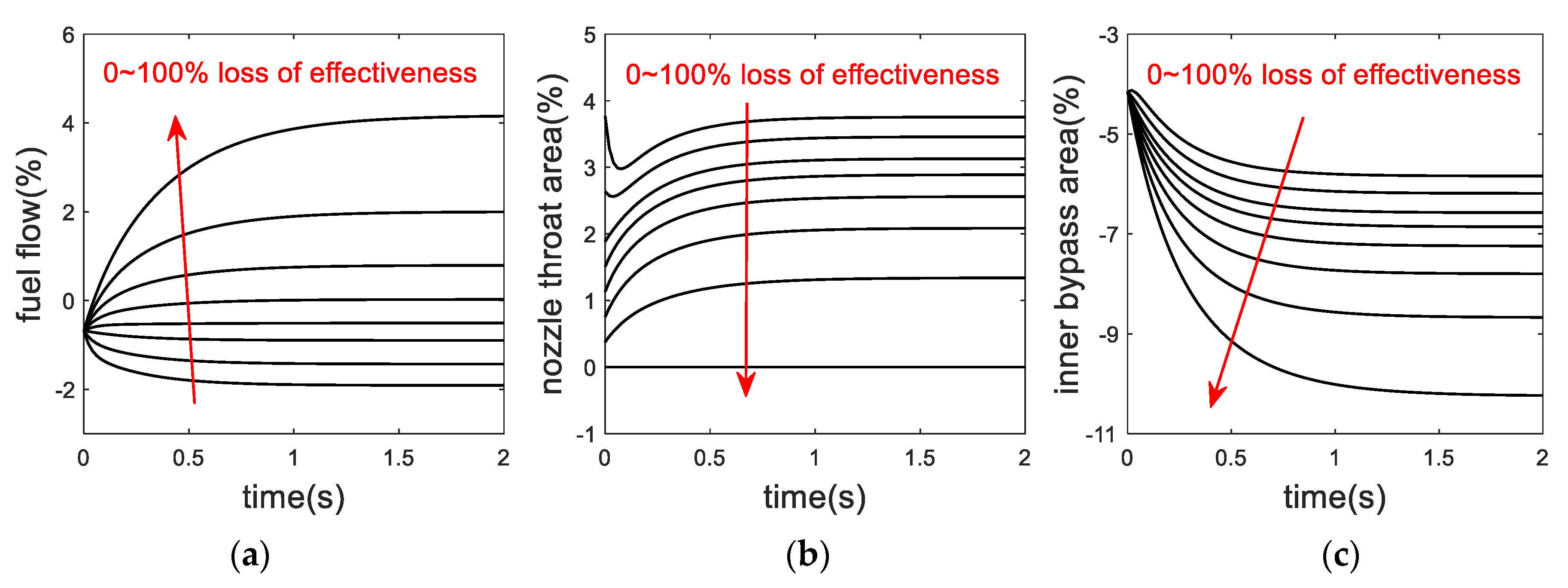
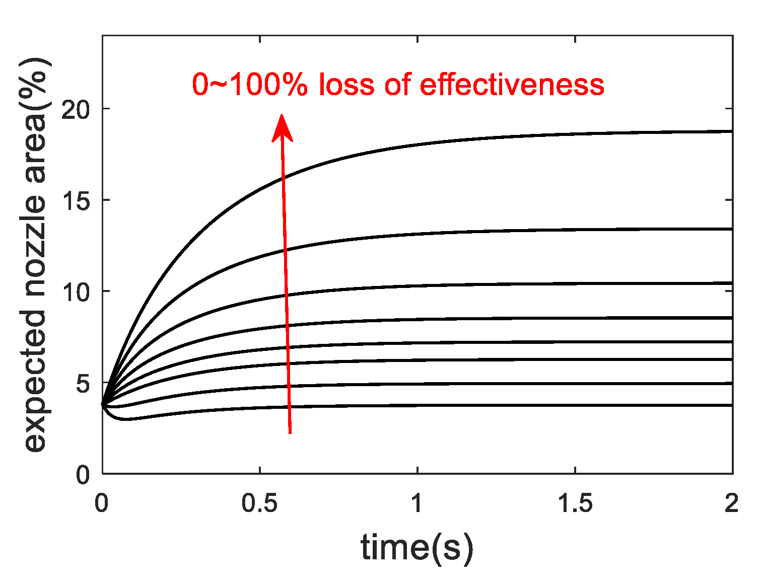
Next, we can verify the fault tolerant ability of the proposed design. Assume that the SMO estimates the effectiveness matrix to be , which means that the actuator still has part of the control effectiveness. Applying the following control instruction: hold constant and increase by 0.1 (a normalized value of 1.85%), the responses of the closed-loop control system under different effectiveness loss conditions ranging from 0~100% are shown in Figure 5 and Figure 6. It can be seen that the FTC design achieves the same control goal in all the faulty situations, even when the actuator totally fails to work. In this case, no longer participates in the control process and the control effect is redistributed to the remaining unfaulty actuators. From Figure 5, it is also seen that as the loss level of effectiveness increases, the controlled variables require more time to settle down. This is due to the discrepancy between the expected control signals and the real control signals. Figure 7 displays the expected that are calculated with the FTC law under all faulty conditions. When the actuator fails, it can no longer complete the expected control task that the controller gives, so the controller has to keep on making adjustments until the control goal is satisfied. The discrepancy becomes bigger as the actuator deteriorates. Usually, it will also lead to a larger variation of the remaining control variables. Similarly, the FTC results can be verified with adaptive SMC design, shown in Figure 8 and Figure 9, which will not be discussed any further here.
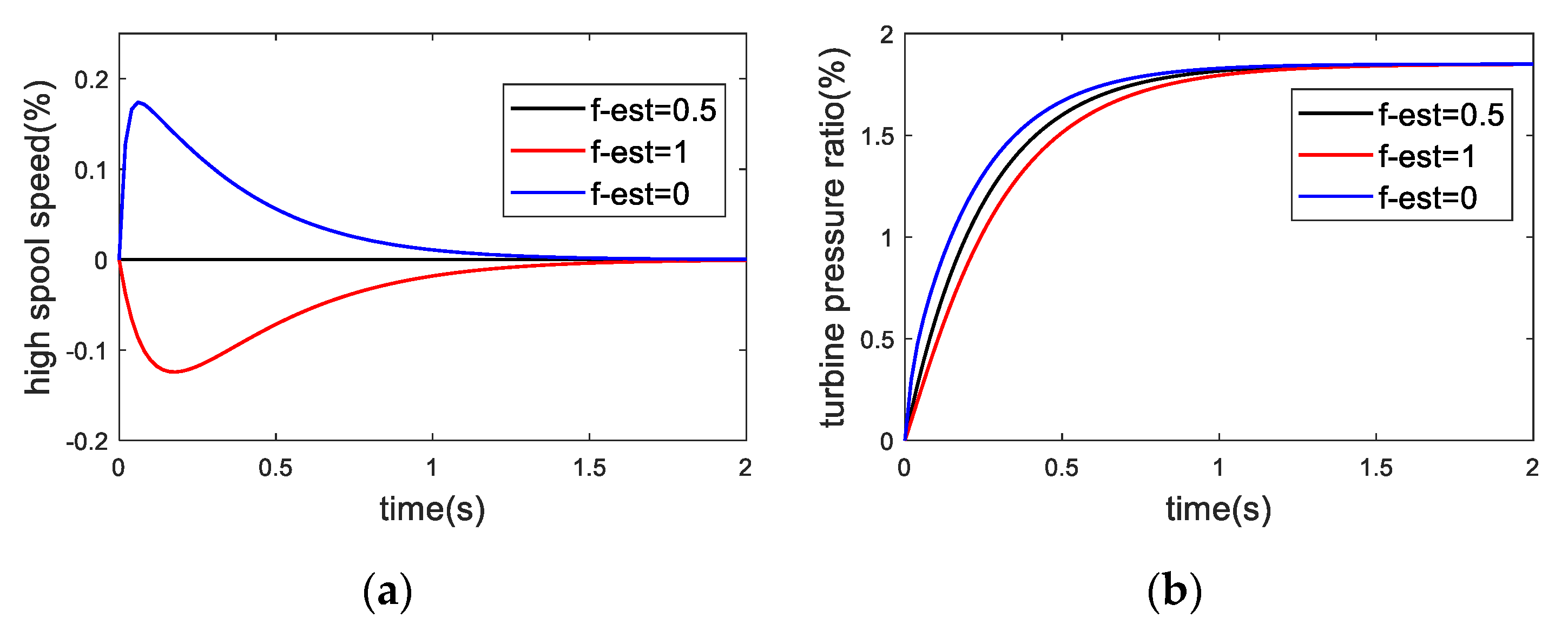
The fault estimation information can have an impact on the fault tolerant control result. Assume the real effectiveness matrix to be , Figure 10a shows the response of controlled variables in different fault reconstruction (FC) situations of . It can be seen that the accurate reconstruction situation produces the minimum variation of the high-pressure spool speed, shown in the black line. This can be explained by the switching function defined in (19). Given the fact that the nonlinear part of the SMC law () takes less part in this simulation compared to the linear part (), so when the reconstruction information is accurate, the derivative of the switching function can be approximated to be:
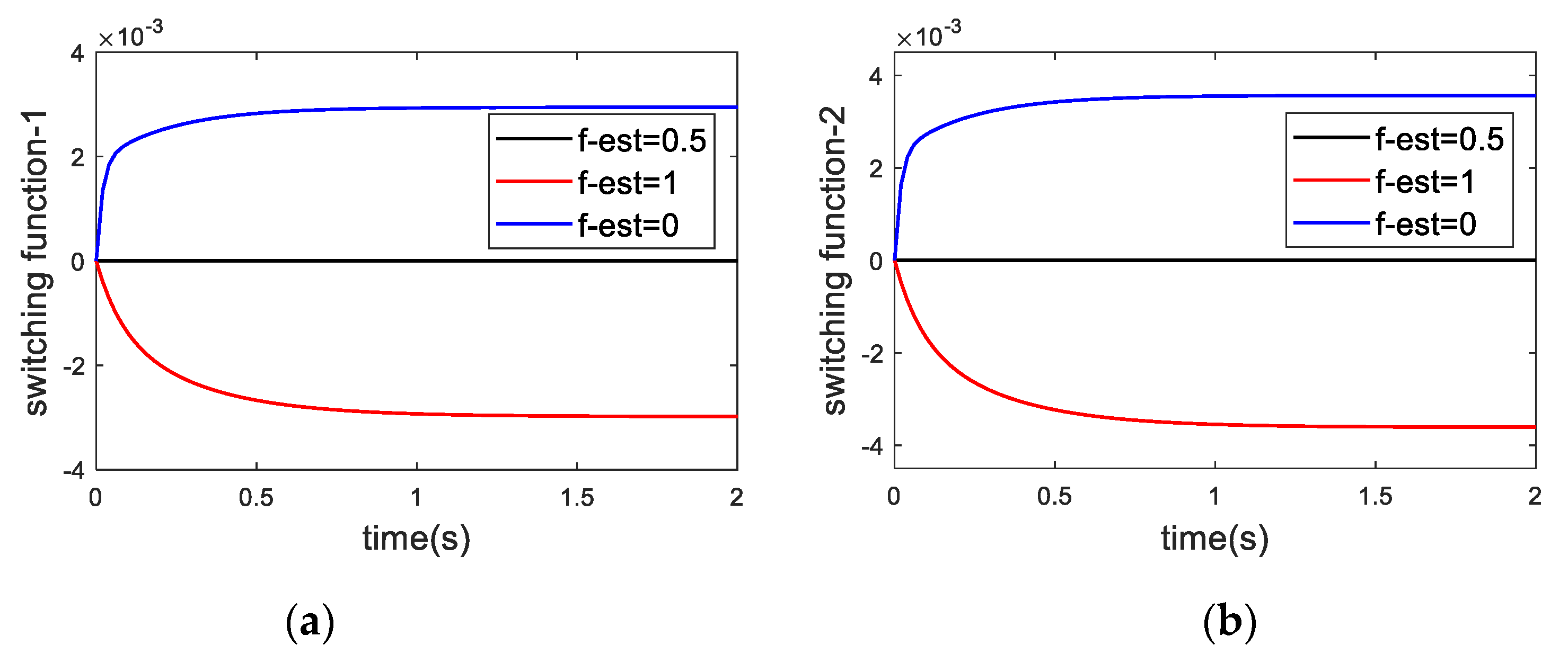
This implies a good sliding performance of the system, which can be demonstrated in Figure 11. As is seen, the value of the switching function in the black line roughly equals zero.
4. Hardware-in-The-Loop Test
The hardware-in-the-loop (HIL) test provides an effective platform by testing actual components of a system along with virtual computer-based simulation models in real time [31,32]. By this means, the test quality is enhanced, the design cycle is shortened and the reliability of the tested components is improved. Here, the “actual component” refers to a distributed control system while the “virtual model” is the component level model of a variable cycle engine. As shown in Figure 12, the distributed control system (DCS) is made up of several intelligent nodes, including the data acquisition nodes, the actuator control nodes, and a core control node. Each of them is an embedded system based on Zynq and communicates with each other through the TTP/C (Time-Triggered Protocol/class C) bus. The VCE model runs on NI-myRIO in real time. The interface simulator can provide an electrical emulation of real sensors’ signals such as the thermal-couple signals of temperature, the piezo-resistance signals of pressure, the linear variable differential transformer (LVDT) signals of actuator displacements and so on. Not merely, it conditions the driving electricity which is produced by the actuator nodes. The operation principle of the platform is as follows: myRIO delivers the engine outputs to the interface simulator, producing relevant sensors’ signals. These signals are collected by corresponding data acquisition nodes in the distributed control system and transmitted to the core control node. The core control node receives commands from the monitor and computes the desired control variables, which are transmitted to actuator control nodes to calculate the driving current. The current is then acquired by the interface simulator, driving the corresponding actuator (which is a model in fact) in myRIO. As a result, the operation of the engine gets updated.
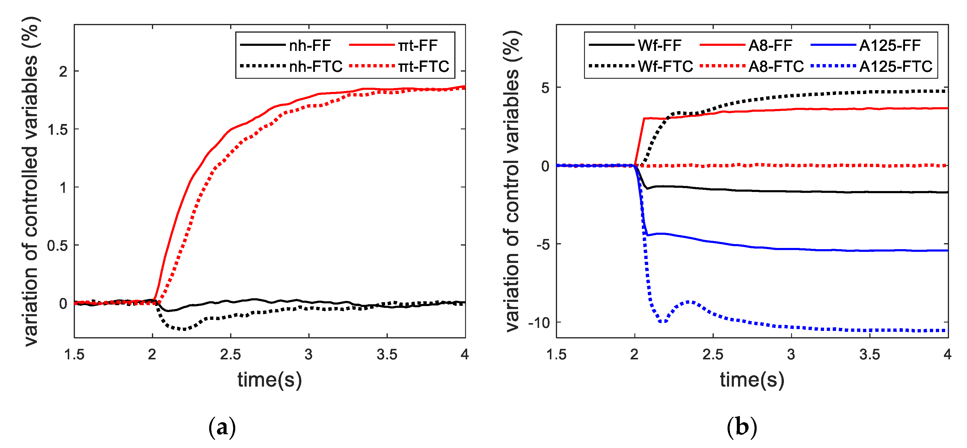
Here we verify the FTC of the proposed design and this is performed by comparing the control results between the fault-free and faulty situations. First, assume that the system is fault-free. At 2 s, the following control instruction is applied: hold constant and increase by 1.85%, we can see in Figure 13a that reaches the set value as expected and remain steady after 1.5 s. The control variables are depicted in Figure 13b where finally drops by 1.71%, increases by 3.65% and reduces by 5.46% in the steady state. Next, suppose that a lock-in-place fault happens to the actuator, which means , and the fault reconstruction method gives an inaccurate estimation, which is . As is seen in Figure 13a, the control goal is realized as well. In the steady state, increases by 4.78%, drops by 10.57% and does not change at all. Compared to the simulation result in Section 3, the curves in the HIL test look rougher. The main reason is that the controlled object here is the component level model of VCE, which possesses more nonlinear characteristics. Moreover, the HIL test involves many characteristics of the real control system, including the actuating property of actuators, the inertia of sensors, the noise of all the electronical components, the stability of the control time cycle, etc. Similar results can be attained with the adaptive method, shown in Figure 14.
Note that although the FTC case reaches the same control goal as the fault-free case, it does not mean that the engine operating conditions in the two cases are totally the same. Figure 15 shows the difference of low-pressure spool speeds between the fault-free and lock-in-place fault condition, and this owes to the difference of the control variables in these two situations.
5. Conclusions
In this paper, a fault tolerant control design addressing the actuator faults of a variable cycle engine is proposed with the sliding mode control scheme. The basic idea of the design is to explore and make use of the functional redundancy brought by the multiple variable geometries in the VCE. The proposed actuator FTC design in this work is divided into two parts: the fault reconstruction part and the fault tolerant control part. In the fault reconstruction part, a sliding mode observer is designed to detect and reconstruct the effectiveness loss of the actuator. On the other hand, in the FTC part, it provides a detailed analysis of an SMC-based FTC scheme, which gives consideration to the inaccurate estimation of the effectiveness loss. Additionally, the existence condition for the proposed FTC design is analyzed. Moreover, the SMC-based FTC design is connected with the control allocation concept and adaptive control concept, which produces the SM-CA design and adaptive SMC design. Afterward, this paper gives a new control plan for the intermediate operation of VCE which uses the FVABI to achieve functional redundancy. On this basis, simulations are carried out to verify the FTC result of the proposed design. First, the fault reconstruction ability of the SMO is verified. Results show that it can roughly reproduce the effectiveness loss of the nozzle throat area actuator. However, there exists an error due to the approximation of the equivalent output injection signal. Second, the fault tolerant ability of the proposed FTC design is verified. Results show that it achieves the same control goal in all the effectiveness loss situations. Similar results can be attained with the ASMC design. Additionally, this paper studies the impact of the fault estimation accuracy on the FTC result and shows that an accurate estimation can lead to a good sliding motion of the system. Finally, an HIL test is conducted to verify the proposed design in a real-time DCS. Results show that the FTC design successfully redistributes the control effort among the remaining unfaulty actuators, and achieves the same control goal as the fault-free situation. This demonstrates its application in the engineering aspect.
In the current work, it only gives a simple trail for the management of the functional redundancy in the VCE. It neither discusses the rationality of the FTC control plan nor talks about more possibilities for handling the redundancy. Another problem that the control system cares about is that whether the control range can be as large as the original fault-free situation when the FTC design is applied. These questions remain to be solved in the future work.
Author Contributions
Conceptualization, T.Z.; Data curation, X.Z.; Formal analysis, Y.Y., Z.L., Z.Z. and X.Z.; Investigation, Y.Y.; Methodology, Y.Y., Z.L. and Z.Z.; Project administration, T.Z.; Resources, Z.L.; Software, Z.Z.; Supervision, T.Z.; Validation, Y.Y.; Writing-original draft, Y.Y.; Writing–review & editing, X.Z. All authors have read and agreed to the published version of the manuscript.
Funding
This work was supported by the National Natural Science Foundation of China (Grant number: 51976089).
Institutional Review Board Statement
Not applicable.
Informed Consent Statement
Not applicable.
Data Availability Statement
The data presented in this study are available on request from the corresponding author.
Conflicts of Interest
The authors declare no conflict of interest.
Appendix A
Proof of Theorem 1.
Define
where , and satisfies
where .
Consider the Lyapunov candidate function:
Taking the derivative
Noting that
Substituting it into (54) and denoting as , there is
Therefore, the error system (11) is quadratically stable. The proof is completed. □
Appendix B
The LQR method determines the virtual control v by solving the following performance index
where , . Then there
where is obtained by solving the algebraic Riccati equation below:
References
- Edwards, C.; Lombaerts, T.; Smaili, H. Fault Tolerant Flight Control. Lecture Notes in Control and Information Sciences; Springer: Berlin, Germany, 2010; Volume 399, 560p. [Google Scholar]
- Zhang, Y.; Jiang, J. Bibliographical review on reconfigurable fault-tolerant control systems. Annu. Rev. Control. 2008, 32, 229–252. [Google Scholar] [CrossRef]
- Rausch, R.; Viassolo, D.; Kumar, A.; Goebel, K.; Eklund, N.; Brunell, B.; Bonanni, P. Towards in-flight detection and accommodation of faults in aircraft engines. In Proceedings of the AIAA 1st Intelligent Systems Technical Conference, Chicago, IL, USA, 20–22 September 2004; p. 6463. [Google Scholar]
- Nyulászi, L.; Andoga, R.; Butka, P.; Főző, L.; Kovacs, R.; Moravec, T. Fault detection and isolation of an aircraft turbojet engine using a multi-sensor network and multiple model approach. Acta Polytech. Hung. 2018, 15, 189–209. [Google Scholar]
- Huang, X.H. Sensor fault diagnosis and reconstruction of engine control system based on auto-associative neural network. Chin. J. Aeronaut. 2004, 17, 23–27. [Google Scholar] [CrossRef] [Green Version]
- Litt, J.S.; Parker, K.I.; Chatterjee, S. Adaptive Gas Turbine Engine Control for Deterioration Compensation Due to Aging. NASA/TM-2003-212607. 2003. Available online: https://archive.org/details/nasa_techdoc_20040001041 (accessed on 10 December 2020).
- Turso, J.; Litt, J. Intelligent, Robust Control of Deteriorated Turbofan Engines via Linear Parameter Varing Quadratic Lyapunov Function Design. In Proceedings of the AIAA 1st Intelligent Systems Technical Conference, Chicago, IL, USA, 20–22 September 2004; pp. 678–691. [Google Scholar]
- Zaccaria, V.; Ferrari, M.L.; Kyprianidis, K. Adaptive Control of Microgas Turbine for Engine Degradation Compensation. J. Eng. Gas Turbines Power 2020, 142, 041012. [Google Scholar] [CrossRef]
- Kawatsu, K.; Tsutsumi, S.; Hirabayashi, M.; Sato, D. Model-based fault diagnostics in an electromechanical actuator of reusable liquid rocket engine. In Proceedings of the AIAA Scitech 2020 Forum, Orlando, FL, USA, 6–10 January 2020; p. 1624. [Google Scholar]
- Wang, R.; Liu, M.; Ma, Y. Fault estimation for aero-engine LPV systems based on LFT. Asian J. Control 2021, 23, 351–361. [Google Scholar] [CrossRef]
- Musgrave, J.L.; Guo, T.H.; Wong, E.; Duyar, A. Real-time accommodation of actuator faults on a reusable rocket engine. IEEE Trans. Control. Syst. Technol. 1997, 5, 100–109. [Google Scholar] [CrossRef]
- Zhang, X.; Liu, Y.; Rysdyk, R.; Kwan, C.; Xu, R. An intelligent hierarchical approach to actuator fault diagnosis and accommodation. In Proceedings of the 2006 IEEE Aerospace Conference, Big Sky, MT, USA, 4–11 March 2006. [Google Scholar]
- Boskovic, J.D.; Jackson, J.A.; Mehra, R.K.; Nguyen, N.T. Multiple-model adaptive fault-tolerant control of a planetary lander. J. Guid. Control Dyn. 2009, 32, 1812–1826. [Google Scholar] [CrossRef]
- Habibi, H.; Nohooji, H.R.; Howard, I. Backstepping Nussbaum gain dynamic surface control for a class of input and state constrained systems with actuator faults. Inf. Sci. 2019, 482, 27–46. [Google Scholar] [CrossRef]
- Chen, H.; Zhou, J.; Zhou, M.; Zhao, B. Nussbaum gain adaptive control scheme for moving mass reentry hypersonic vehicle with actuator saturation. Aerosp. Sci. Technol. 2019, 91, 357–371. [Google Scholar] [CrossRef]
- Ahmed Ali, S.; Guermouche, M.; Langlois, N. Fault-tolerant control based super-twisting algorithm for the diesel engine air path subject to loss-of-effectiveness and additive actuator faults. Appl. Math. Model. 2015, 39, 4309–4329. [Google Scholar] [CrossRef]
- Trinh, H.A.; Truong, H.V.A.; Ahn, K.K. Fault Estimation and Fault-Tolerant Control for the Pump-Controlled Electrohydraulic System. Actuators 2020, 9, 132. [Google Scholar] [CrossRef]
- Shin, D.; Moon, G.; Kim, Y. Design of reconfigurable flight control system using adaptive sliding mode control: Actuator fault. Proc. Inst. Mech. Eng. Part G J. Aerosp. Eng. 2005, 219, 321–328. [Google Scholar] [CrossRef]
- Alwi, H.; Edwards, C. Fault tolerant control using sliding modes with on-line control allocation. Automatica 2008, 44, 1859–1866. [Google Scholar] [CrossRef] [Green Version]
- Chen, L.; Edwards, C.; Alwi, H.; Sato, M. Flight evaluation of a sliding mode online control allocation scheme for fault tolerant control. Automatica 2020, 114, 108829. [Google Scholar] [CrossRef]
- Wang, B.; Zhang, Y. An adaptive fault-tolerant sliding mode control allocation scheme for multirotor helicopter subject to simultaneous actuator faults. IEEE Trans. Ind. Electron. 2018, 65, 4227–4236. [Google Scholar] [CrossRef] [Green Version]
- Patel, H.R.; Wilson, D. Parametric Cycle Analysis of Adaptive Cycle Engine. In Proceedings of the 2018 Joint Propulsion Conference, Cincinnati, OH, USA, 9–11 July 2018; p. 4521. [Google Scholar]
- Palman, M.; Leizeronok, B.; Cukurel, B. Mission Analysis and Operational Optimization of Adaptive Cycle Microturbofan Engine in Surveillance and Firefighting Scenarios. J. Eng. Gas Turbines Power 2019, 141, 011010. [Google Scholar] [CrossRef] [Green Version]
- Bringhenti, C.; Barbosa, J.R. Methodology for gas turbine performance improvement using variable-geometry compressors and turbines. Proc. Inst. Mech. Eng. Part A J. Power Energy 2004, 218, 541–549. [Google Scholar] [CrossRef]
- Simmons, R.J. Design and Control of a Variable Geometry Turbofan with and Independently Modulated Third Stream. Ph.D. Thesis, The Ohio State University, Columbus, OH, USA, 2009. [Google Scholar]
- Edwards, C.; Spurgeon, S.K.; Patton, R.J. Sliding mode observers for fault detection and isolation. Automatica 2000, 36, 541–553. [Google Scholar] [CrossRef]
- Tan, C.P. Sliding Mode Observers for Fault Detection and Isolation. Ph.D. Thesis, University of Leicester, Leicester, UK, 2002. [Google Scholar]
- HäRkegåRd, O.; Glad, S.T. Resolving actuator redundancy—Optimal control vs. control allocation. Automatica 2005, 41, 137–144. [Google Scholar] [CrossRef]
- Farkas, B.; Wegner, S.A. Variations on Barbălat’s Lemma. Am. Math. Mon. 2016, 123, 825–830. [Google Scholar] [CrossRef] [Green Version]
- Kurzke, J. GasTurb—The Gas Turbine Performance Simulation Program; GasTurb GmbH: Aachen, Germany, 2012. [Google Scholar]
- Salehi, A.; Montazeri-Gh, M. Design and HIL-based verification of the fuel control unit for a gas turbine engine. Proc. Inst. Mech. Eng. Part G J. Aerosp. Eng. 2020, 234, 1460–1470. [Google Scholar] [CrossRef]
- Yuan, Y.; Zhao, Z.; Zhang, T. A mimicking technique of back pressure in the hardware-in-the-loop simulation of a fuel control unit. Simulation 2020, 96, 375–385. [Google Scholar] [CrossRef] [Green Version]
Figure 1.
Faults in a control system.

Figure 2.
Structure of the actuator fault tolerant control design.

Figure 3.
Schematic diagram of the variable cycle engine.

Figure 4.
Actuator effectiveness reconstruction result of the observer.

Figure 5.
Fault tolerant control (FTC) result of sliding mode control (SMC) design-controlled variables. (a) (b) .
Figure 5.
Fault tolerant control (FTC) result of sliding mode control (SMC) design-controlled variables. (a) (b) .

Figure 6.
FTC result of SMC design-control variables. (a) (b) A8 (c) A125.

Figure 7.
Expected nozzle throat area of in SMC design.

Figure 8.
FTC result of adaptive SMC (ASMC) design-controlled variables. (a) (b) .

Figure 9.
FTC result of ASMC design-control variables. (a) (b) A8 (c) A125.

Figure 10.
FTC result in different fault reconstruction (FC) situations. (a) controlled variables (b) control variables.
Figure 10.
FTC result in different fault reconstruction (FC) situations. (a) controlled variables (b) control variables.

Figure 11.
Switching function in different FC situations. (a) first term (b) second term.

Figure 12.
Hardware-in-the-loop simulation platform. ① Interface simulator ② Distributed controller ③ myRIO (Engine CLM) ④ Monitor.
Figure 12.
Hardware-in-the-loop simulation platform. ① Interface simulator ② Distributed controller ③ myRIO (Engine CLM) ④ Monitor.

Figure 13.
FTC result of SMC design in hardware-in-the-loop (HIL) test. (a) controlled variables (b) control variables.
Figure 13.
FTC result of SMC design in hardware-in-the-loop (HIL) test. (a) controlled variables (b) control variables.

Figure 14.
FTC result of ASMC design in HIL test. (a) controlled variables (b) control variables.

Figure 15.
Comparison of low spool speeds in the HIL test.

Publisher’s Note: MDPI stays neutral with regard to jurisdictional claims in published maps and institutional affiliations. |
© 2021 by the authors. Licensee MDPI, Basel, Switzerland. This article is an open access article distributed under the terms and conditions of the Creative Commons Attribution (CC BY) license (http://creativecommons.org/licenses/by/4.0/).
Share and Cite
MDPI and ACS Style
Yuan, Y.; Zhang, T.; Lin, Z.; Zhao, Z.; Zhang, X. Actuator Fault Tolerant Control of Variable Cycle Engine Using Sliding Mode Control Scheme. Actuators 2021, 10, 24. https://0-doi-org.brum.beds.ac.uk/10.3390/act10020024
AMA Style
Yuan Y, Zhang T, Lin Z, Zhao Z, Zhang X. Actuator Fault Tolerant Control of Variable Cycle Engine Using Sliding Mode Control Scheme. Actuators. 2021; 10(2):24. https://0-doi-org.brum.beds.ac.uk/10.3390/act10020024
Chicago/Turabian StyleYuan, Yuan, Tianhong Zhang, Zhonglin Lin, Zhiwen Zhao, and Xinglong Zhang. 2021. "Actuator Fault Tolerant Control of Variable Cycle Engine Using Sliding Mode Control Scheme" Actuators 10, no. 2: 24. https://0-doi-org.brum.beds.ac.uk/10.3390/act10020024
Note that from the first issue of 2016, this journal uses article numbers instead of page numbers. See further details here.