
Pressure Estimation Based on Vehicle Dynamics Considering the Evolution of the Brake Linings’ Coefficient of Friction

1
School of Automotive Studies, Tongji University, Shanghai 201804, China
2
Institute of Intelligent Vehicle, Clean Energy Automotive Engineering Center, Tongji University, Shanghai 201804, China
*
Author to whom correspondence should be addressed.
Actuators 2021, 10(4), 76; https://0-doi-org.brum.beds.ac.uk/10.3390/act10040076
Submission received: 18 March 2021
/
Revised: 2 April 2021
/
Accepted: 6 April 2021
/
Published: 8 April 2021
(This article belongs to the Special Issue Actuators for Intelligent Electric Vehicles)
Abstract
:To mitigate the issue of low accuracy and poor robustness of the master cylinder pressure estimation (MCPE) of the electro-hydraulic brake system (EHB) by adopting EHB’s own information, a MCPE algorithm based on vehicle information considering the evolution of the brake linings’ coefficient of friction (BLCF) is proposed. First, the MCPE algorithm was derived combining the vehicle longitudinal dynamics and the wheel dynamics, in which the inertial measurement unit (IMU) was adopted to adapt the MCPE algorithm to road slope change. In order to estimate the brake pressure accurately, the driving resistance of the vehicle was obtained through a vehicle test under coasting condition. After that, with the active braking function of EHB, the evolution of the BLCF was acquired through extensive real vehicle test under different initial temperatures, different initial vehicle speeds, and different brake pressures. According to the test results, a revised model of the BLCF is proposed. Finally, the performance of the MCPE based on the revised BLCF model was compared with that based on a fixed BLCF model. Vehicle test demonstrates that the former MCPE algorithm is not only more accurate at low vehicle speed than the later, but also robust to road slope change.
1. Introduction
With the development of electric and intelligent vehicles, the conventional brake system (i.e., vacuum booster) cannot meet the new demands any more, and the brake by wire system (BBW) came into being. BBW cannot only maximize the recovery of braking energy through coordinated control with the driven motor for electric vehicles, but for intelligent vehicles, it can also realize high-performance active braking, which is the development trend of automotive brake systems in the future [1,2]. As a branch of BBW, the electro-hydraulic brake system (EHB), which is based on a hydraulic system and activated by electric motors, is superior to the electro-mechanical brake system (EMB) in production inheritance and security reliability [3,4,5,6,7,8,9,10,11,12].
Pressure control is the core technology of EHB and has been extensively studied [13,14,15,16]. However, as far as the author knows, in addition to some research by the author’s team [17,18,19], all the master cylinder pressure control algorithms in the existing literature adopted the master cylinder pressure sensor as the feedback signal for closed-loop control. The existence of the pressure sensor increased the cost and the risk of sensor failure. As one of the key safety components of automobiles, once the pressure sensor fails, the function of EHB will be seriously affected. Some products adopted two pressure sensors in the master cylinder for mutual inspection as a solution of failure detection and backup, which led to a further increase in cost [20]. For this reason, master cylinder pressure estimation (MCPE) is a promising solution to the above-mentioned problems. In addition, the motor information of EHB (e.g., motor torque, motor rotational angle, etc.) can increase the possibility of MCPE.
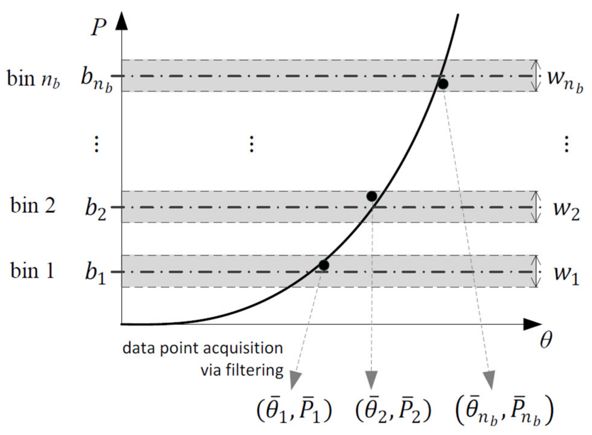
The MCPEs in literatures were mainly based on the relationship between the master cylinder piston position (which can be obtained from the motor rotational angle and the transmission ratio of the reduction mechanism) and the master cylinder pressure. A first-order polynomial, a second-order polynomial, and a look-up table were used to render the pressure–position relationship in [16,21,22], respectively. However, due to the hysteresis and time-varying characteristics of the pressure–position relationship, the above methods were not accurate all the time. For this reason, the extended least squares and the recursive least squares were adopted to update the coefficients of the quadratic polynomial in [23,24], respectively. In [18], the coefficients were further reduced to one and updated by the recursive least squares with a fixed forgetting factor. Although the above algorithms can adjust the pressure–position model online, the coefficients of the polynomials fluctuate violently during the adaptive process due to the significant uncertainty of EHB (e.g., temperature, motor speed, brake pads wear, and so on). Once the pressure sensor fails, the values of coefficients at that moment are fixed for MCPE, resulting in an inaccurate pressure estimation with large uncertainty. Furthermore, if the EHB is only operated within a small pressure region, the pressure–position model may be over-fitted to this region. This would be a common occurrence in road vehicles since most instances of braking in daily driving involve only low decelerations. To this end, Ref. [25] proposed a bin-least-square algorithm, in which the measured (θ, P) data points were allocated according to the P value into nb “bins”, each of which corresponded to a small window of P. These windows were non-overlapping and distributed over the operating range of P as shown in Figure 1. The data points allocated to each bin were aggregated over time into single θ and P values; the (θ, P) pairs from all nb bins were then imported to the least square algorithm. Although this method improved the stability of polynomial coefficients, it also deteriorated the accuracy of MCPE by reducing the sensitivity of polynomial coefficients to system pressure-position uncertainty.
It is worth pointing out that all the above MCPE algorithms were based on the pressure sensors and cannot be used in EHB unequipped with pressure sensors. To this end, Ref. [26] proposed an interconnected pressure estimation method in which the key characteristic parameter of the pressure–position curve, namely, the nonlinearly parameterized perturbations, could be estimated via EHB’s dynamics based on the LuGre friction model. The problem is that the friction itself in EHB is time-varying, and this method needs to be demonstrated through extensive real vehicle verifications in the future.
The above-mentioned methods considered only the actuator characteristics (e.g., pressure–position model, friction model of EHB) and depended on the model accuracy. Inspired by the wheel cylinder pressure estimation algorithms [27], Ref. [28] proposed a MCPE algorithm based on vehicle longitudinal dynamics and wheel dynamics for the first time. Real vehicle test demonstrated that the MCPE outperformed that proposed in [26]. However, the brake linings’ coefficient of friction (BLCF) was regarded as constant. In fact, the BLCF is greatly affected by vehicle speed, brake pressure and brake linings’ temperature [29].
Summarized by the above literature, the MCPE for EHB requires further improvement on accuracy and robustness, and the BLCF needs to be studied further. Two main contributions make this work distinctive from the previous studies: (1) the MCPE in [28] has been expanded in this article to adapt it to more working conditions, such as slope condition, based on inertial measurement unit (IMU), which is easily accessible for vehicles equipped with an electronic stability control system (ESC); (2) a revised model of BLCF is proposed based on extensive real vehicle tests, which contributes to a more accurate MCPE. The rest of this article is organized as follows. The vehicle platform and the EHB prototype under consideration are introduced in Section 2. The MCPE is proposed based on the longitudinal dynamics of the vehicle in Section 3. The driving resistance is tested through real vehicle tests in Section 4. The effect of different initial temperatures, different brake pressures, and different initial vehicle speeds on the BLCF is studied through extensive real vehicle tests, and a revised model of the BLCF is proposed in Section 5. Real vehicle tests under normal driving conditions, including flat road and slope road, are conducted to verify the proposed MCPE in Section 6. Section 7 concludes this article.
2. Test Vehicle and the EHB Prototype
2.1. Test Vehicle
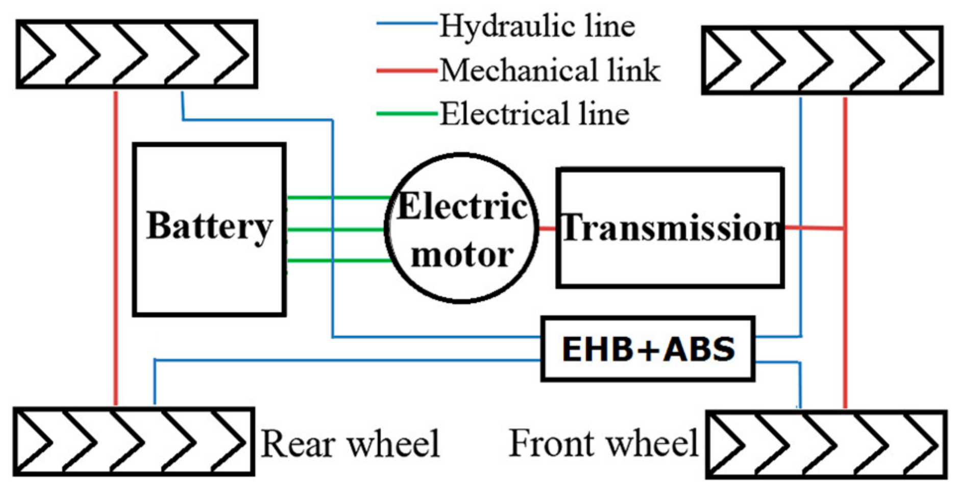
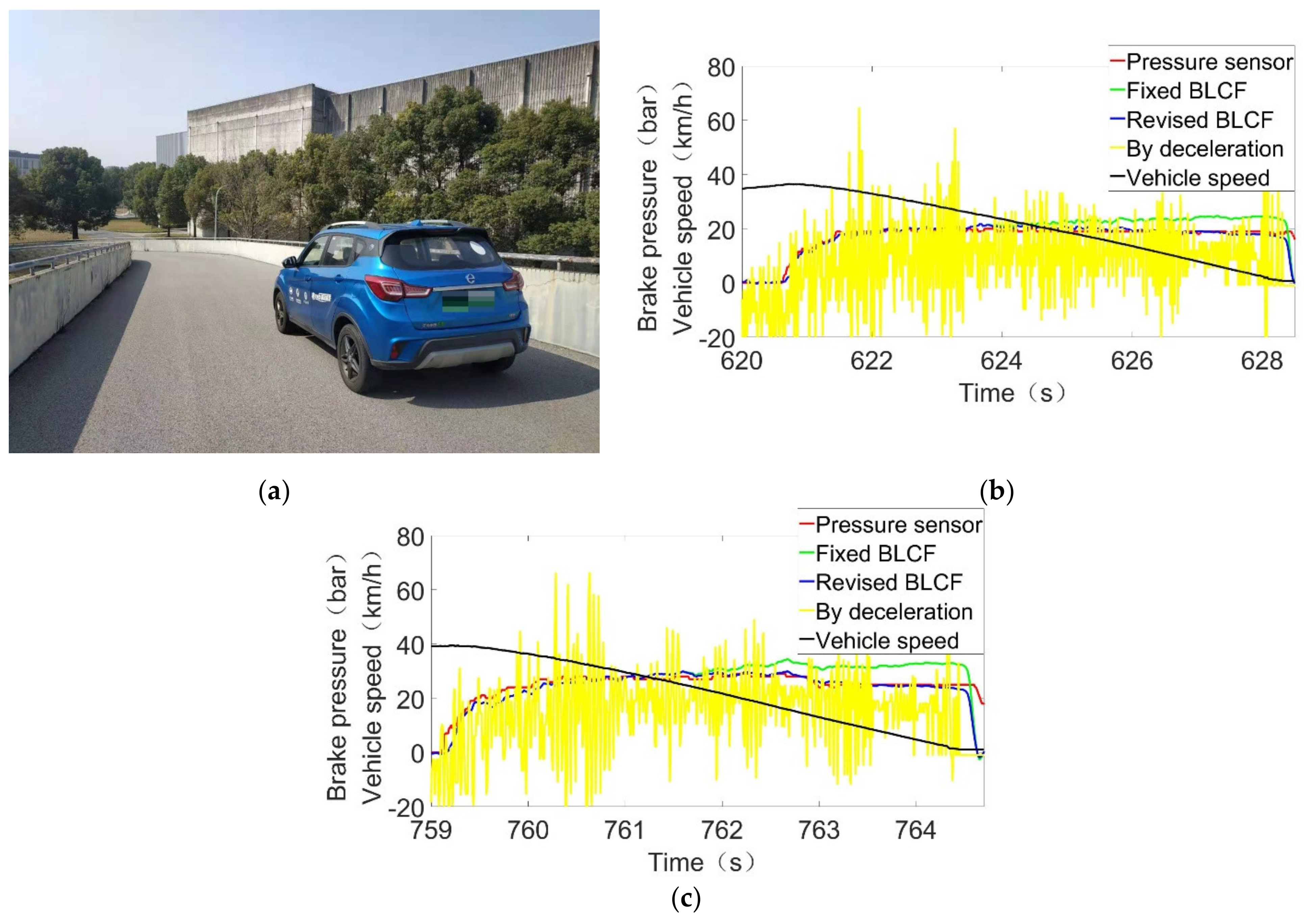
A front-wheel-drive electric vehicle equipped with EHB is selected as the test vehicle, as shown in Figure 2. In this work, the regenerative brake function of the driven motor was invalid in braking, and all the braking force was supplied by the EHB. The test vehicle was equipped with the anti-lock brake system (ABS) and an additional IMU needed to be installed on the test vehicle.
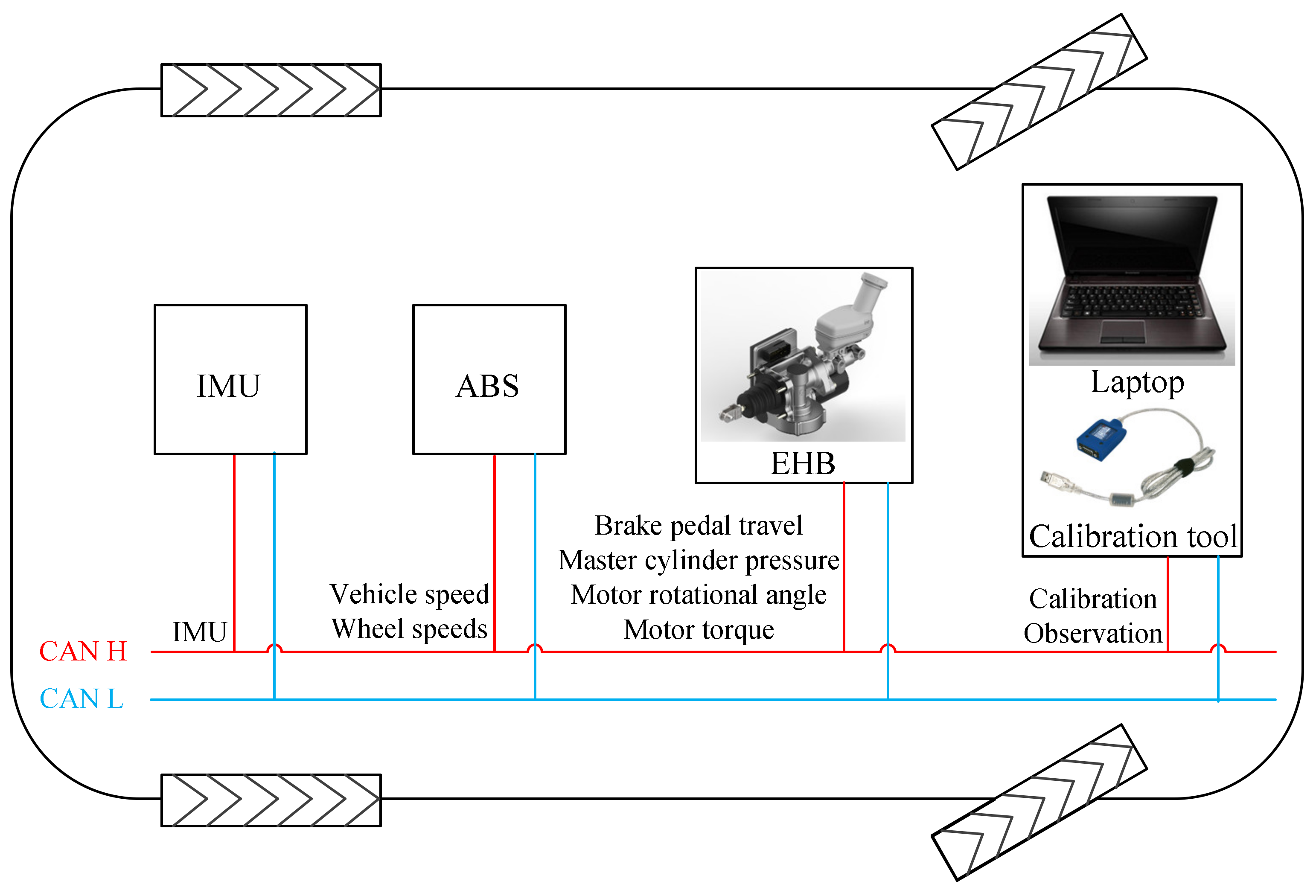
The scheme of the vehicle platform is displayed in Figure 3; messages could be transferred from one node to another through controller area network (CAN). The electric control unit (ECU) of EHB received signals from the ABS, IMU, and sensors equipped in EHB and generated the control demand to the electric motor of EHB, which drove the reduction gear that directly pushed the master cylinder to generate pressure. A laptop was used for online calibration and observation via corresponding tools. There were two working modes of EHB: normal mode and X-by-wire mode. In normal mode, the EHB tracked the target pressure generated by the brake pedal, while in the X-by-wire mode, the EHB tracked the target pressure generated by the laptop.
2.2. EHB Prototype
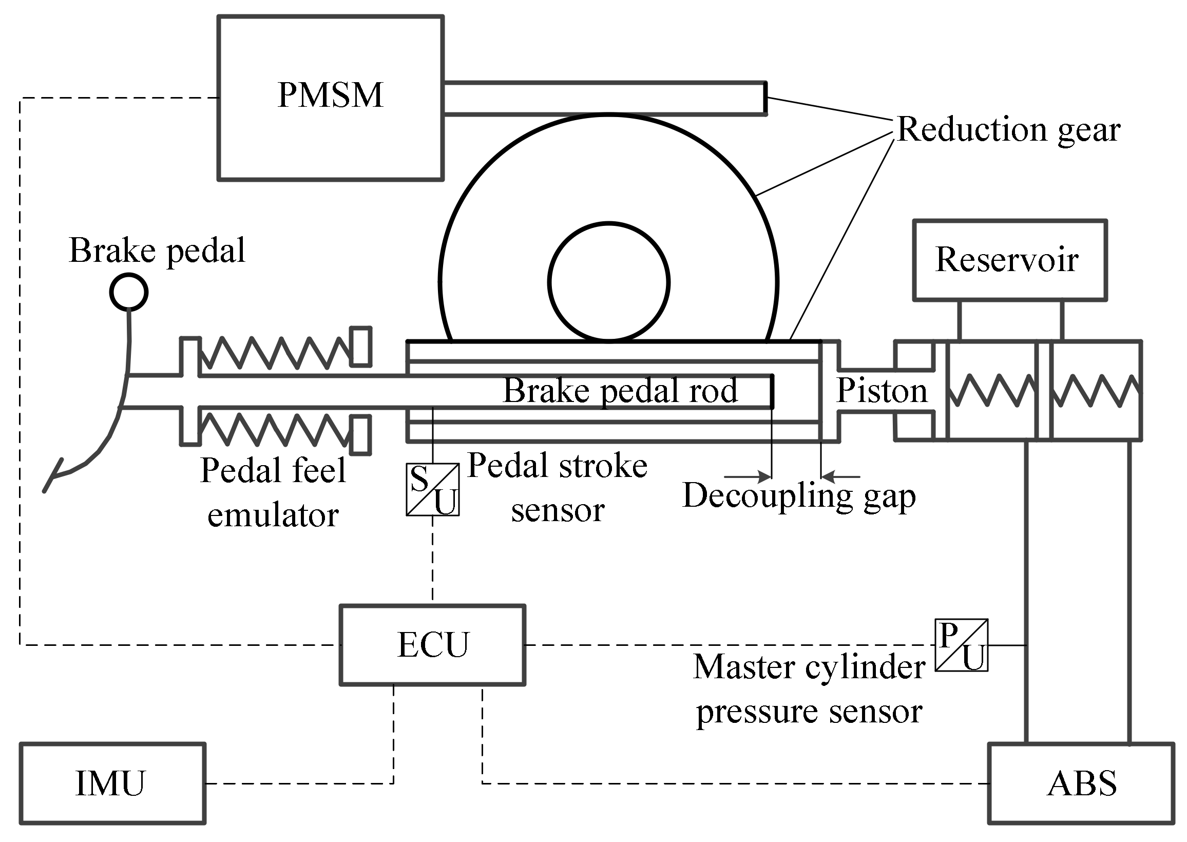
The scheme of EHB is shown in Figure 4. The EHB consisted of four parts: brake pedal unit, motor driven unit, brake execution unit, and ECU. The brake pedal unit, which included a brake pedal and a pedal feel simulator, provided the driver with a good pedal feel. The motor driven unit was the power source of the system, including a permanent magnet synchronous motor (PMSM) and reduction gear. The brake execution unit had the same structure as the conventional hydraulic brake system and included the master cylinder, the brake pipelines, and the ABS. A decoupling gap was designed to realize system decoupling, that is, the brake pedal and the master cylinder were not directly connected. In normal mode, the driver depressed the brake pedal, and the brake pedal rod compressed the pedal feel emulator to generate a brake feel. ECU analyzed the driver’s braking intention according to the pedal stroke signal and controlled the PMSM to generate corresponding torque; therefore, there was no mechanical connection between the brake pedal and the master cylinder [12]. The pressure sensor was adopted as a feed-back signal for master cylinder pressure control and played no role in MCPE.
3. MCPE Algorithm Design
3.1. Assumptions
In this work, the following assumptions are considered:
- This work investigates the MCPE in the ordinary braking scenarios. The ABS must not work;
- The master cylinder pressure is the same as the wheel cylinder pressure. In other words, the pressure wave propagation dynamics are ignored;
- In the vehicle longitudinal dynamics, the longitudinal tire slip ratio is ignored;
- The vehicle mass is assumed to be known or could be obtained by using the estimation method during the acceleration process [30];
- The vehicle lateral dynamics are ignored.
3.2. MCPE Based on Vehicle Longitudinal Dynamics
Under braking conditions, the vehicle longitudinal dynamics can be expressed by Equation (1) [32].
where denotes the vehicle mass, ; denotes the vehicle rotational mass, ; denotes the vehicle longitudinal deceleration, ; denotes the braking force, ; denotes the rolling resistance, ; denotes the wind resistance, ; denotes the slope resistance, , as shown in Figure 5.
The vehicle longitudinal dynamics of Equation (1) already include the wheel rotational dynamics so the braking force of each wheel can be expressed by Equation (2).
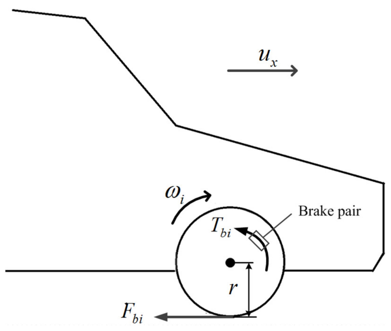
where the subscript () denotes the front left wheel, the front right wheel, the rear left wheel, and the rear right wheel, respectively. denotes the braking torque of a certain wheel, ; denotes the wheel rolling radius, , as shown in Figure 6.
The braking torque of each wheel can be expressed by Equation (3).
where denotes the pressure of the hydraulic circuit, ; , and denote the wheel cylinder piston area, the BLCF, and the effective friction radius of each wheel, respectively. Both and are constant. To simplify the problem, a new variable is defined to render the characteristic of BLCF as Equation (4).
where denotes the pressure–torque factor of each wheel, .
Substituting Equations (2)–(4) into Equation (1), the pressure can be calculated by Equation (5):
Some variables in Equation (5) can be further expressed as follows:
where denotes the acceleration of gravity, ; denotes the road slope, ; denotes the rolling resistance coefficient.
The signal of the IMU can be expressed by Equation (8) according to its working principle.
A new variable is defined to render the equivalent characteristic of all the BLCFs as Equation (9).
Substituting Equations (6), (8), and (9) into Equation (5), the MCPE algorithm can be expressed as follows:
It should be noted that renders all the rotational mass of the vehicle, which mainly includes the wheels and the rotor of the driven motor, so it can be expressed by Equation (11).
where denotes the moment of inertia of a single wheel, ; denotes the moment of inertia of the driven motor’s rotor, ; and denote the transmission ratio and transmission efficiency of the vehicle transmission system. Table 1 provides the specifications of the test vehicle, in which all the vehicle parameters have been calibrated off line.
According to Equation (11) and Table 1, we see that , so the value of is too small to be ignored compared to . Furthermore, the signal of , which is obtained by vehicle speed or wheels speeds, is full of noise [28]. Considering the above reasons, is ignored in Equation (11), and the MCPE algorithm is finally designed as follows:
According to Equation (12), in order to estimate the brake pressure, we must first determine , i.e., the driving resistance, and , i.e., the sum of the pressure–torque factors of all wheels.
4. Driving Resistance
Driving resistance of the vehicle, including the rolling resistance and the wind resistance, can be expressed as follows:
The driving resistance is affected by the slope. In fact, the slope of normal road is not large, that is, . Therefore, the influence of slope change on driving resistance is ignored.
Driving resistance is generally obtained through real vehicle tests. Under the coasting condition, the vehicle longitudinal dynamics can be expressed by Equation (14).
Substituting Equation (8) into Equation (14) and ignoring , driving resistance can be acquired by Equation (15).
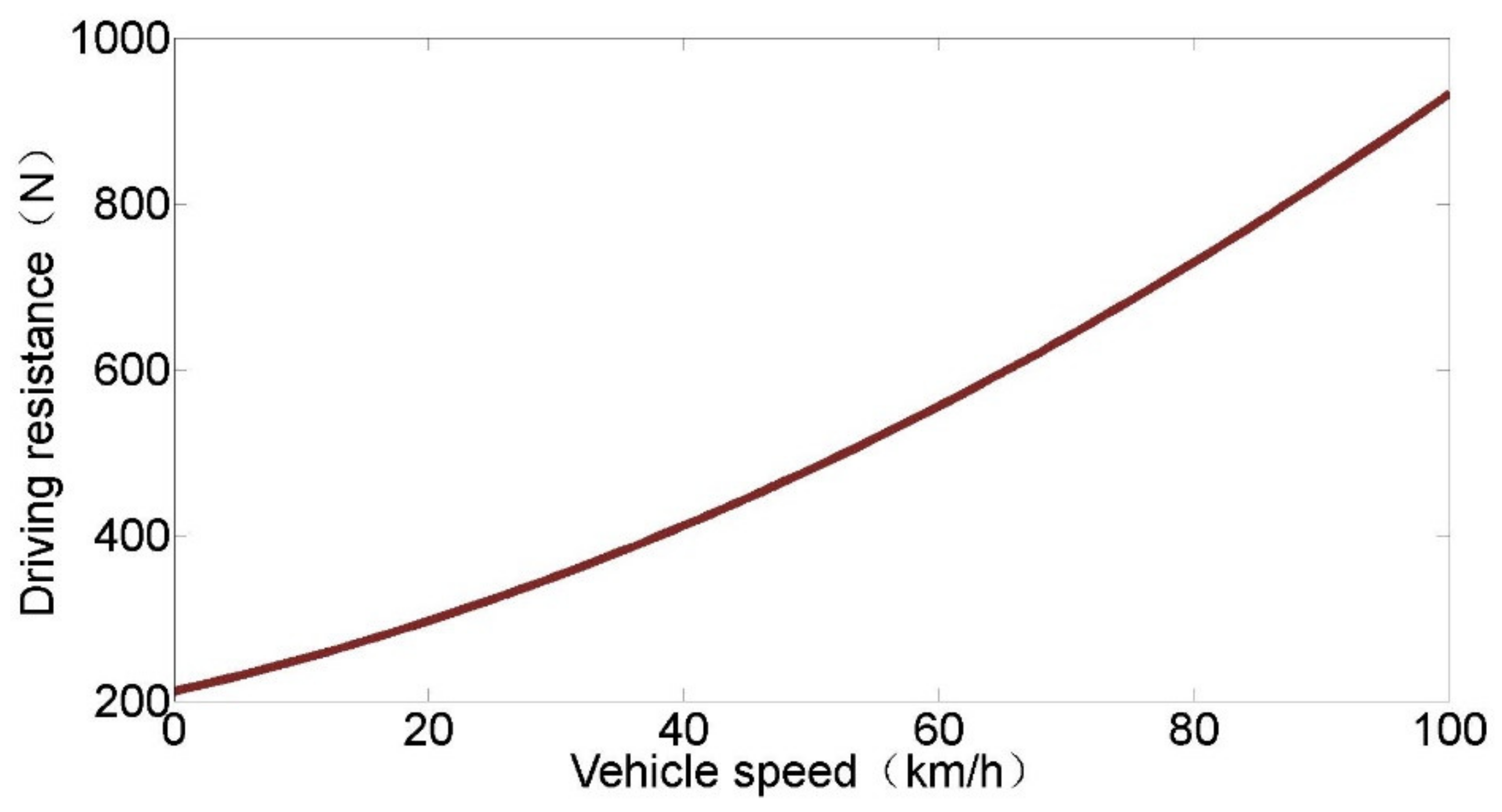
Generally, a special road is required to conduct the coasting test. Due to the limitation of test conditions, this article adopted the method of segmented testing, that is, the coasting test was broken down into multiple different vehicle speed segments to be tested separately, and finally, the test data are integrated and fitted by a quadratic polynomial, as shown in Figure 7.
The analytical model of the driving resistance is shown in Equations (16) and (17).
where denotes the vehicle speed, .
5. Revised Model of the BLCF
The BLFC has been widely studied in literature and is affected by several phenomena: fading [33,34]; bedding [35]; hysteresis against the pressure [36]; hysteresis against the speed [37], wear [38,39], and aging [35]; and variation in the environmental conditions [40]. The behavior of a pad–disc coupling is also dependent on the chemical composition and mechanical properties of each component [41]. Therefore, the BLCF can range between 0.3 and 0.6 [41,42], with peaks up to 0.8 and down to 0.1 [36,43].
There are mainly two methods in the literature to estimate the BLCF:
- Model based analytical approach: which strives for a physical understanding and analytical description of the friction behavior. Accurate BLCF models usually incorporate a temperature model, which is solved by the finite element method (FEM). However, owing to the high computational burden, it is not possible to use this approach for an online estimation of the brake temperature. For this reason, it is not feasible to use the FEM, along with a friction model, for estimation purposes [43,44,45].
- Neural-networks: which found an extensive application in friction modelling in recent years due to the capability of accurately modeling complex nonlinear phenomena with several inputs. The main limitation of the neural-network approach is the high experimental burden for the training/learning processes. Furthermore, the approach based on the neural-network is purely black box; therefore, it is not able to describe the actual phenomenology of the tribological contact [46,47,48].
The most recent research put forth a semi-empirical dynamic model of BLCF resulting from a thorough experimental campaign conducted on a brake dynamometer. The model rendered the rotor speed, rotor temperature, and contact area dynamics by means of a set of three differential equations and validated for three passenger cars’ brake systems [29]. Though the state-of-the-art BLCF model can account for several tribological phenomena, parameter calibration requires lots of experiments.
As far as the author knows, all the above-mentioned methods are based on brake dynamometers, in other words, none of them are based on vehicle test. Furthermore, in normal braking conditions, the variation range of influencing factors of BLCF, such as temperature, may not be that large.
In this article, to estimate brake pressure, needs to be identified. Although is the sum of the pressure–torque factor of all wheels and not the same as BLCF of each wheel, can render the equivalent characteristics of sum of the front and rear BLCFs for both and , which are constant. In this sense, and BLCF have similarities in characteristics. Therefore, the characteristics of BLCF can also be used to explain and analyze the characteristics of .
According to Equation (12), can be measured by the following equation based on a vehicle test:
where the brake pressure can be obtained by pressure sensor. When is 0, the above equation diverges so that the value of is set to not less than 2 bar.
5.1. Error Analysis
There are two things to point out: (1) is ignored in Equation (12). (2) is also ignored in Equation (15) when identifying the driving resistance. That is, the ignored is balanced in Equations (12) and (18). In other words, Equations (12) and (18) are the exact formula to calculate and , respectively.
Table 2 and Table 3 provide the specifications of the IMU and the master cylinder pressure sensor, respectively.
It can be roughly calculated from the sensors’ specifications that the error between the calculated by Equation (18) and the actual value should be within ±1.8%.
5.2. The Effect of Temperature on
5.2.1. The Effect of Initial Disc Temperature on the Evolution of
Although there are many factors affecting BLCF, the most important are the temperature, brake pressure, and vehicle speed [29]. During the braking process, kinetic energy of the vehicle is converted into heat, and the temperature of the friction pair rises sharply. For organic friction material, which is the most widely used in brakes at present, the BLCF increases first and then decreases with disc temperature. The turning point (critical temperature) varies with different specific ingredients and their ratio. The experimental results in Ref. [49] show that the critical temperature of BLCF under different Sb2S3 and ZrSiO4 ratios ranges from 230 °C to 330 °C. Other literature shows that the critical temperature of BLCF is generally around 230 °C [29,50]. For the friction material of the test vehicle in this article, the author only knows that it is organic friction material, but the specific composition and ratio are difficult to find due to proprietary reasons.
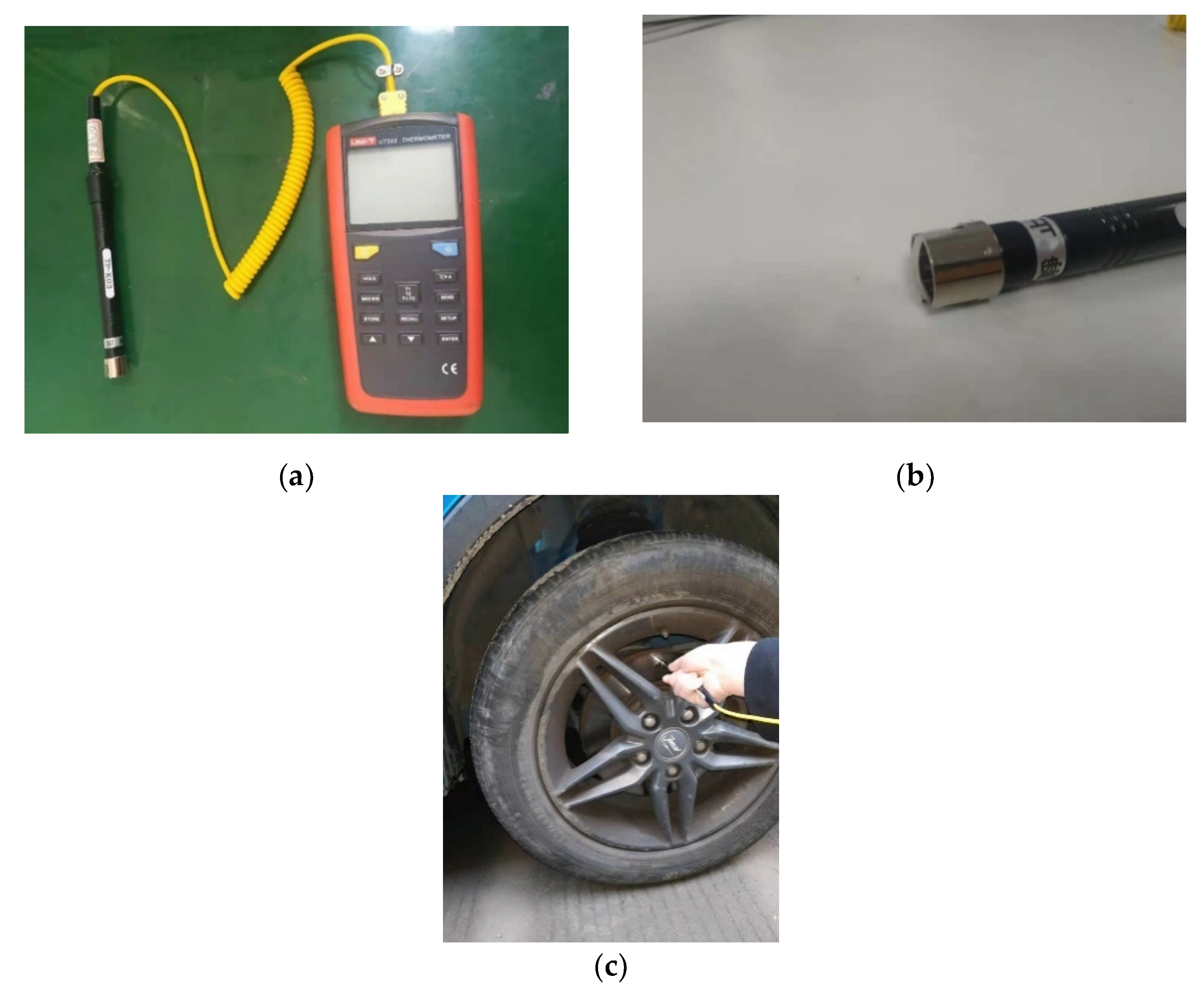
In this work, a contact temperature sensor was adopted to measure the disc’s temperature, as shown in Figure 8. When the vehicle was static, the probe of the temperature sensor was touched to the surface of the brake disc, and the temperature on the display instrument was stable in 3–5 s.
The test process was as follows: when the vehicle was static, we, first, measured the temperature of the brake discs, then, accelerated the vehicle to a predetermined speed, and finally, braked. The temperature could only be measured when the vehicle was static. Therefore, we tried to speed up the vehicle as quickly as possible in the test to reduce the temperature change during this period. Six groups of tests with different initial temperatures of the brake discs were conducted, as shown in Table 4. Test results (i.e., evolution of ) are shown in Figure 9.
In Figure 9a, stayed around zero at the beginning when there was no brake pressure and quickly dropped and converged to a negative value after the vehicle speed was reduced to zero, which verifies the correctness of Equation (18) and the accuracy of driving resistance identification. When braking, rose quickly and converged, indicating that there was a small delay between the brake pressure and the vehicle deceleration (50–100 ms). When braking under a constant pressure, became larger and larger with time because the temperature of the friction pair rose sharply (but did not reach the critical temperature). In addition, the decrease in vehicle speed during braking also led to an increase in , which was the so called “Stribeck” effect.
We heated the brake disc by repeated accelerations and brakings; the temperature of the disc was increased. Figure 9b–f show the constant pressure braking test with the initial vehicle speed of 65–80 km/h and the brake pressure of 35–60 bar, but the initial braking temperature is different. We can conclude that, when the initial temperature of the brake disc is within 130 °C, the temperature has little effect on the evolution of , but the effect is greater when the temperature is above 200 °C, where the temperature of the brake pair reaches the critical value. In addition, the violent fluctuation between 5000 and 5000.5 s in Figure 9b was caused by the speed bump on the road.
5.2.2. Statistics of Initial Disc Temperature
Although the effect of temperature on was studied in Section 5.2.1, the temperature of the brake disc is usually not very high in practice. Generally speaking, the thermal balance of the brake disc is maintained at about 100 °C during low-intensity braking, which is common in city driving conditions [48,50,51].
Additionally, this article recorded statistics of the front brake disc temperature at the end of several regular driving trips, as shown in Figure 10. Due to the different driving styles of the drivers, the most “prudent” driver and the most “adventurous” driver were selected for testing. The results are shown in Table 5 and Table 6.
The temperature of the brake disc after each trip was related to the driving style, traffic condition, and ambient temperature. Most of the statistics were within 130 °C and the average was about 90 °C.
It can be concluded from the above that the influence of the initial disc temperature on the evolution of can be ignored under normal driving conditions.
5.3. The Effect of Brake Pressure on
The influence of brake pressure on the BLCF was related to the material of the friction pair, and specific tests were required. Ref. [52] pointed out that, for organic friction materials, BLCF first increases and then decreases with the increase of brake pressure; for powder metallurgy friction materials, BLCF decreases with the increase of braking pressure.
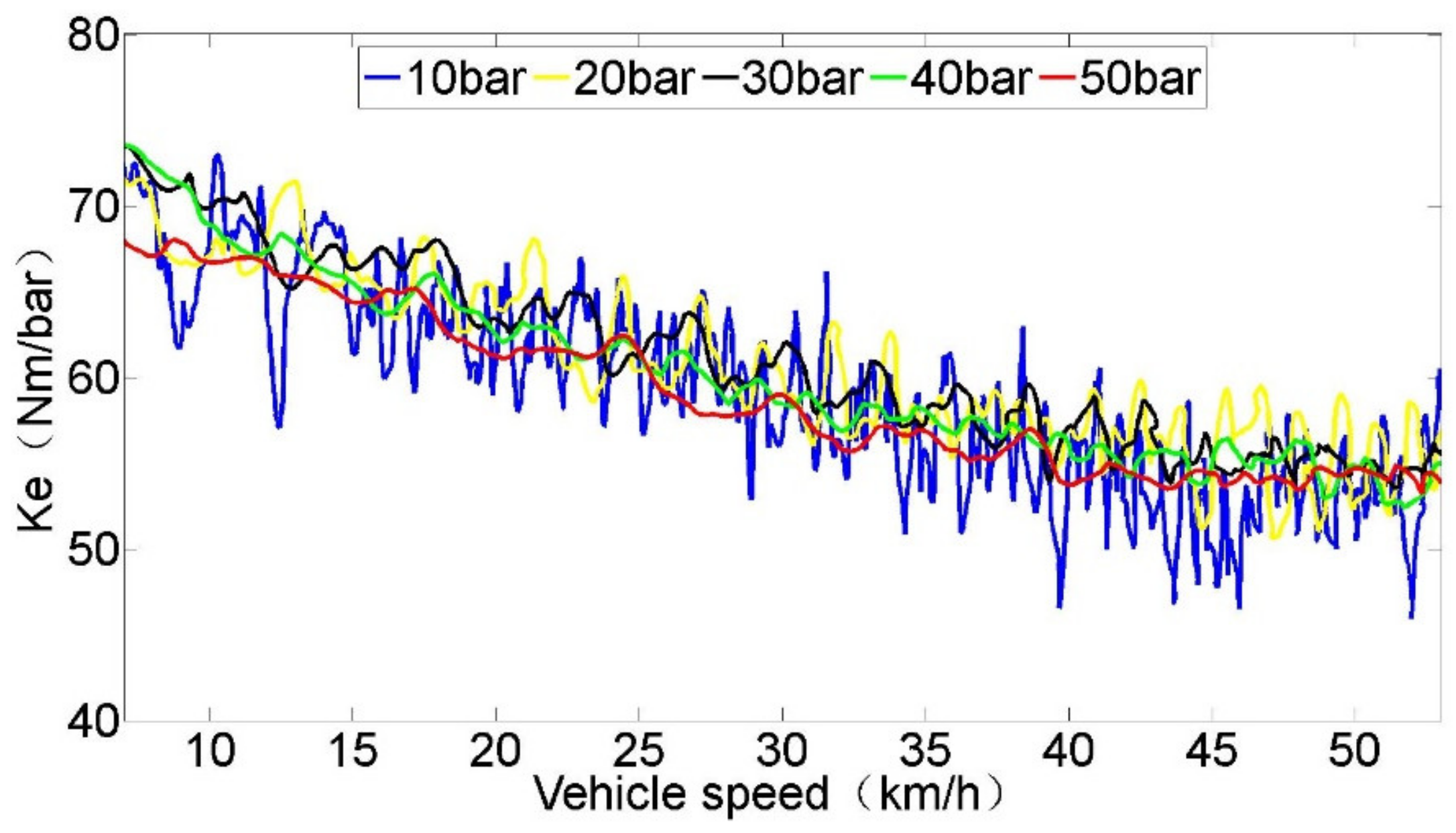
This article carried out tests with initial vehicle speed of 60 km/h and brake pressure of 10 bar, 20 bar, 30 bar, 40 bar, and 50 bar based on the X-by-wire function of EHB. The initial temperature of the brake disc was set to 90 °C each time at the beginning of the test. The test results are shown in Figure 11.
From the perspective of the entire vehicle speed range, the average value of first increased and then decreased with the increase of brake pressure, but the overall change was not large (especially within the range of normal brake pressure). Therefore, the effect of brake pressure on is ignored in this article.
5.4. The Effect of Vehicle Speed on
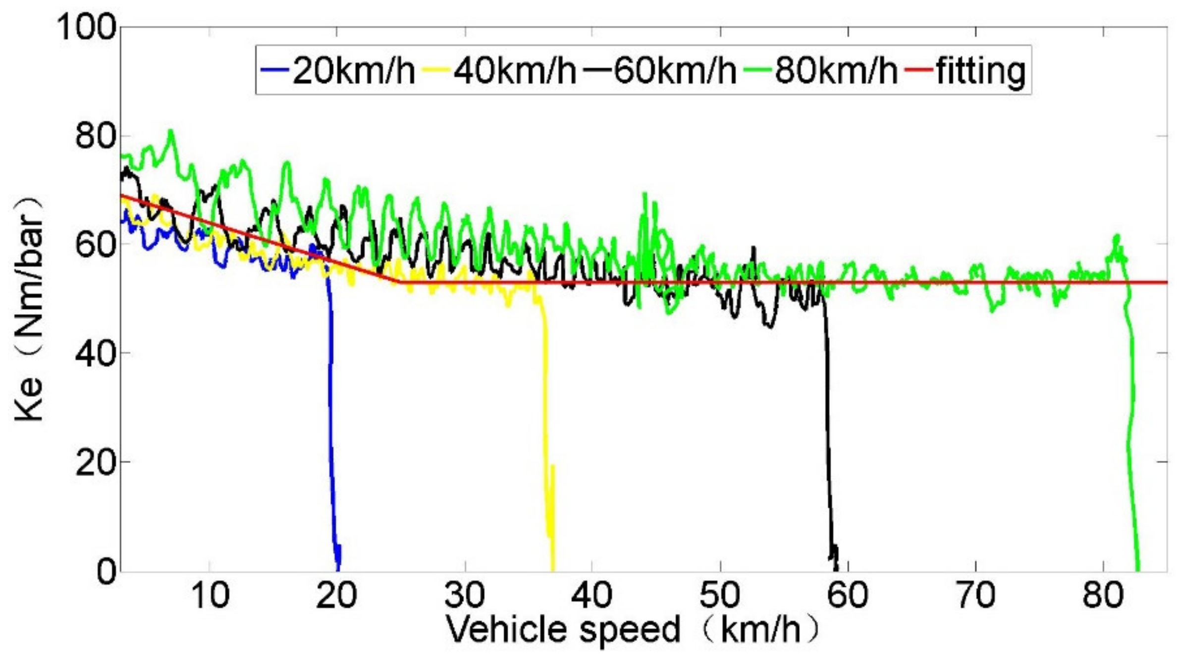
The BLCF was affected by the speed of the vehicle and obeyed the Stribeck characteristic [53,54,55,56], that is, the BLCF was greatly affected by speed.
Under normal driving conditions, the brake pressure was within 30 bar. Vehicle tests with the brake pressure of 15 bar and initial vehicle speed of 20 km/h, 40 km/h, 60 km/h, and 80 km/h were carried out based on the X-by-wire function of EHB with initial disc temperature of 90 °C. Test results are shown in Figure 12.
had a Stribeck effect with the vehicle speed and increased when the vehicle speed was under the critical speed. Specifically, the critical speed was about 30 km/h, 45 km/h and 60 km/h with the initial vehicle speed of 40 km/h, 60 km/h, and 80 km/h, respectively (phenomenon 1). The evolution of with different initial vehicle speeds did not coincide. The greater the initial vehicle speed, the greater the at the end of braking (phenomenon 2).
The explanation of the above two phenomena is that the temperature of the friction pair increased during braking (especially when the initial braking speed was high), which made the BLCF increase. The conclusion in Section 5.2 “The influence of the initial temperature on the evolution of under normal driving conditions is negligible” is based on the condition “at the same initial vehicle speed”. However, when the initial vehicle speed is different, due to the different braking temperature evolution in the process, even if the initial temperature is the same, the evolution of will be different.
It should be noted that, in normal driving conditions, it is rare to decelerate the vehicle from 80 km/h to zero all at once. The more common situation is to decelerate the vehicle from “80 km/h to 60 km/h”, from “60 km/h to 40 km/h”, from “40 km/h to 20 km/h”, and from “20 km/h to zero” in a braking process. From this point of view, the revised BLCF model was defined as a piecewise linear function according to the trend of in the above several speed ranges. That is, when the vehicle speed was lower than a certain critical speed, increased as the vehicle speed decreased; when the vehicle speed was above the critical speed, was fixed, as shown in Equation (19).
where denotes the critical vehicle speed, ; denotes the when the vehicle speed is zero, ; denotes the when the vehicle speed exceeds the critical speed, .
There was a certain degree of subjectivity when dividing the speed zone. In addition, defining the revised BLCF model as a piecewise linear function approximated the test results. Based on the above reasons, the three parameters in Equation (19) can be calibrated more accurately in real vehicle tests. The calibration result of this article is shown in Equation (20).
6. MCPE Based on the Revised BLCF Model
6.1. Flat Road
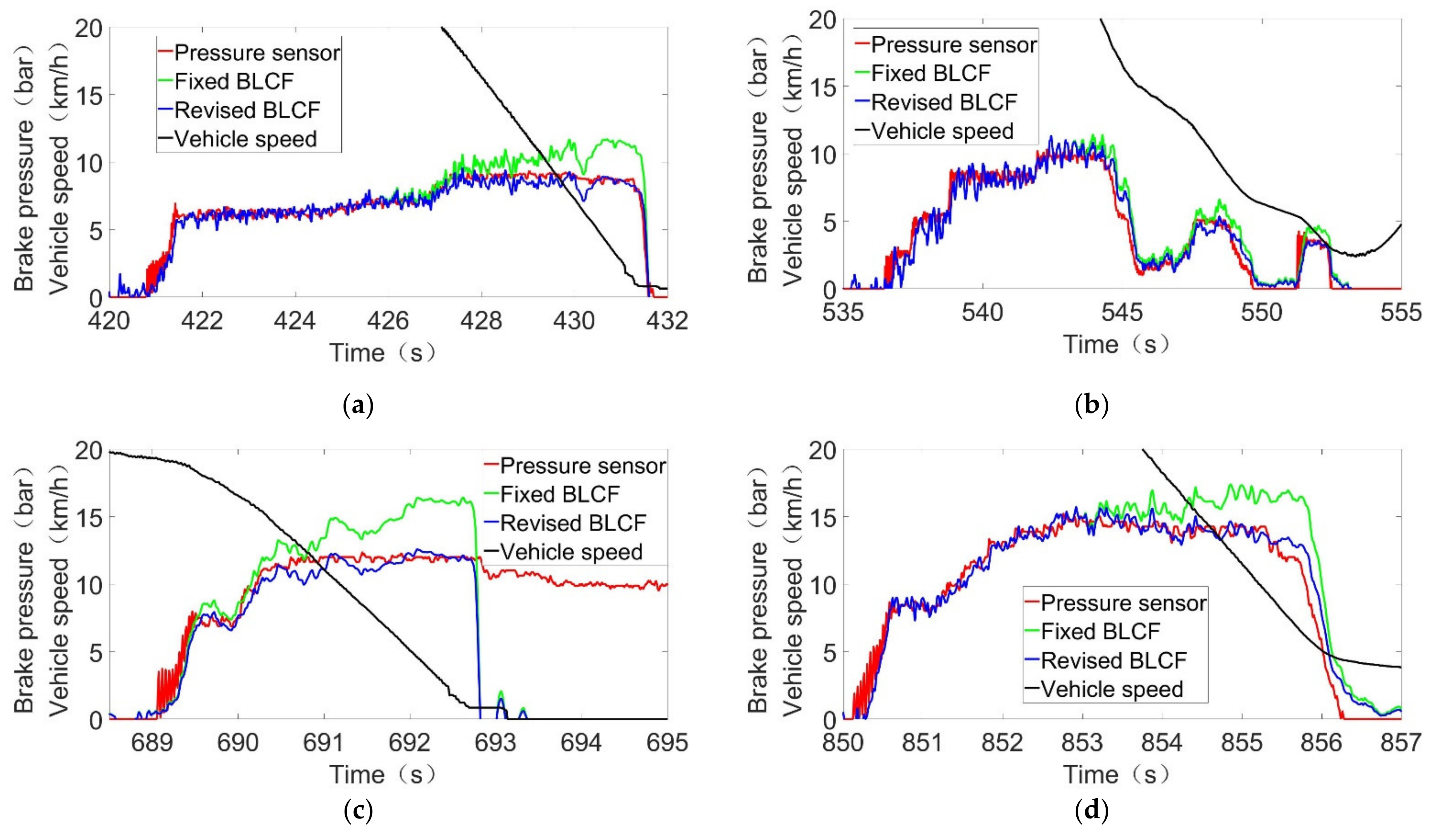
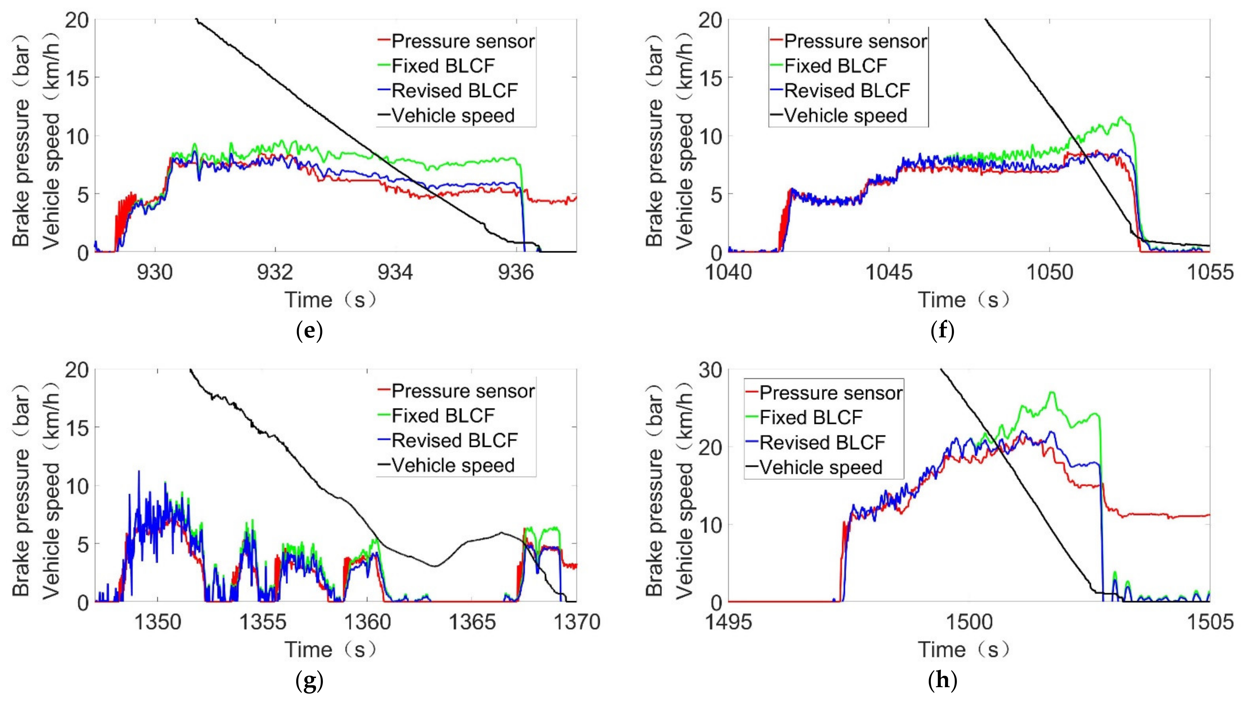
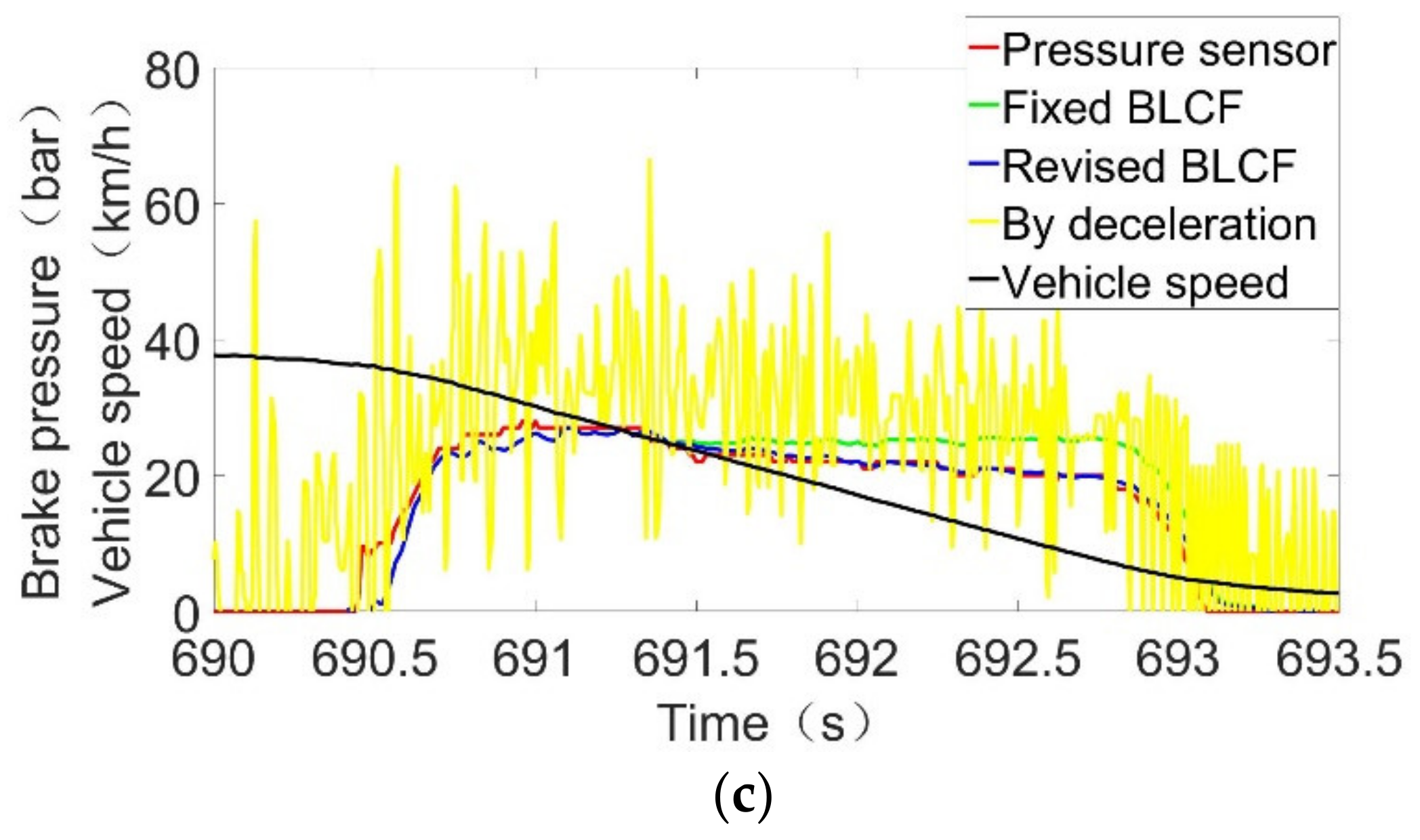
The master cylinder pressure can be estimated by Equations (12) and (20). The MCPE was verified by real vehicle tests under normal driving conditions. In order to highlight the superiority of the revised BLCF model, it was compared with the fixed BLCF (). Test results are shown in Figure 13. In the legend, “fixed BLCF” refers to “pressure estimated based on fixed BLCF model”, and the legend “revised BLCF” refers to “pressure estimated based on revised BLCF model” in Figure 13.
Thanks to the revised model of BLCF, the pressure estimation algorithm proposed in this article was much more accurate when the vehicle speed is low, and the root mean square error (RMSE) was 0.9182 bar. It was much smaller than 1.8248 bar of the MCPE with a fixed BLCF model.
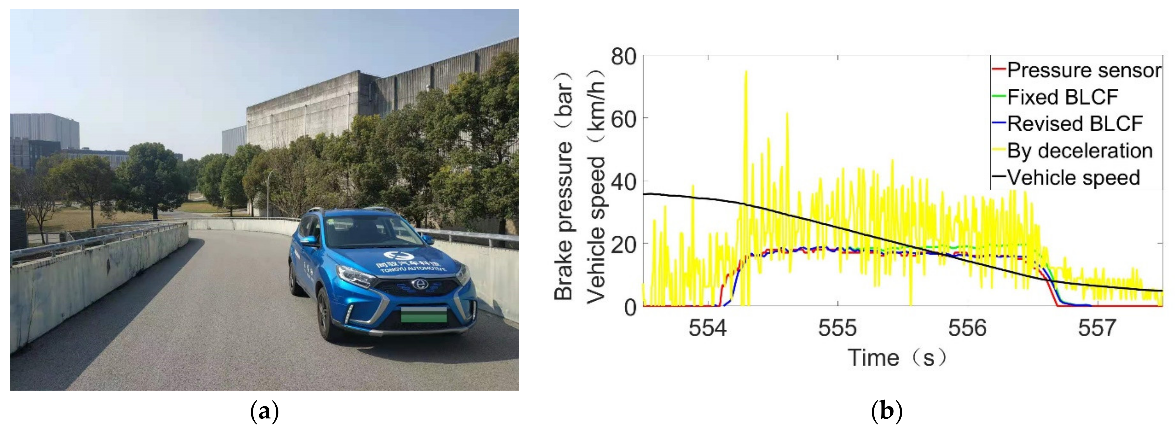
6.2. Slope Road
Section 6.1 proves the superiority of the MCPE based on revised BLCF model, while this section tries to prove slope adaptability of the proposed method.
The MCPE algorithm, based on longitudinal deceleration, which ignored the road slope, can be expressed by Equation (21) as proposed in [28].
Vehicle tests were conducted on a road with slope of 5.5°; test results are shown in Figure 14 and Figure 15.
The error between the MCPE based on vehicle longitudinal deceleration and the actual pressure can be derived by comparing Equations (21) and (12):
We could conclude from Equation (22) that the estimated pressure was higher than the actual pressure when the vehicle was going uphill and lower than the actual pressure when the vehicle was going downhill, which was consistent with the test results. Furthermore, the error was greatly affected by the slope; even a slope of 5.5° could cause a pressure estimation error of about 9 bar. In addition, the deceleration signal was obtained from the difference between the vehicle speeds at different times and fluctuated sharply, which led to a lot of noise in the estimated pressure.
7. Conclusions
Aiming at the problems of low accuracy and poor robustness of the MCPE algorithm, based on EHB’s own sensor information, a MCPE algorithm based on vehicle information is proposed. Compared with the existing literature, the innovation of this article lies in the fact that the BLCF is affected by temperature, brake pressure, and vehicle speed. Additionally, a revised BLCF model is proposed based on a thorough experimental campaign, which is finally verified by real vehicle tests. Compared with the MCPE based on a fixed friction factor, the accuracy is greatly improved. In addition, by adopting IMU information, pressure can be accurately estimated on slopes. In short, the proposed MCPE algorithm can provide EHB with an accurate, robust feedback signal that can be used for pressure control, which can save EHB costs and reduce the risk of pressure sensor failure.
Future works can further study how to integrate different pressure estimation algorithms, such as the MCPE proposed in this work and the MCPEs based on EHB’s own information, to further improve the accuracy and robustness of the MCPE algorithm. Furthermore, the effect of the variability of disc thickness, block thickness, etc. on and the MCPE, can be studied in future works.
Author Contributions
Conceptualization, B.S.; Data curation, B.S.; Formal analysis, B.S.; Funding acquisition, L.X. and Z.Y.; Investigation, B.S.; Methodology, B.S.; Project administration, L.X. and Z.Y.; Resources, B.S.; Software, B.S.; Supervision, L.X. and Z.Y.; Validation, B.S.; Visualization, B.S.; Writing—original draft, B.S.; Writing—review and editing, B.S. All authors have read and agreed to the published version of the manuscript.
Funding
This research was funded by the Research on Development of Electronic Control Chassis System and Active Control Technology (Grant No. 20511104601).
Institutional Review Board Statement
Not applicable.
Informed Consent Statement
Not applicable.
Data Availability Statement
Detailed data are contained within the article. More data that support the findings of this study are available from the author B.S. upon reasonable request.
Acknowledgments
The authors are thankful for the support of the School of Automotive Studies and the IIV (Institute of Intelligent Vehicle) of Tongji University and Tongyu Automobile Technology Co., Ltd.
Conflicts of Interest
The authors declare no conflict of interest.
Abbreviations
| MCPE | Master cylinder pressure estimation |
| EHB | Electro-hydraulic brake system |
| BLCF | Brake linings’ coefficient of friction |
| IMU | Inertial measurement unit |
| BBW | Brake by wire system |
| ESC | Electronic stability control system |
| ABS | Anti-lock brake system |
| CAN | Controller area network |
| ECU | Electric control unit |
| PMSM | Permanent magnet synchronous motor |
| FEM | Finite element method |
References
- Schenk, D.E.; Wells, R.L.; Miller, J.E. Intelligent Braking for Current and Future Vehicles. Int. Congr. Expo. 1995. [Google Scholar] [CrossRef]
- Jonner, W.; Winner, H.; Dreilich, L.; Schunck, E. Electrohydraulic Brake System-The First Approach to Brake-by-Wire Technology. SAE Trans. 1996, 105, 1368–1375. [Google Scholar] [CrossRef]
- Reuter, D.F.; Lloyd, E.W.; Zehnder, J.W.; Elliott, J.A. Hydraulic Design Considerations for EHB Systems. Braking Syst. 2003. [Google Scholar] [CrossRef]
- D’alfio, N.; Morgando, A.; Sorniotti, A. Electro-hydraulic brake systems: Design and test through hardware-in-the-loop simulation. Veh. Syst. Dyn. 2006, 44, 378–392. [Google Scholar] [CrossRef]
- Sorniotti, A.; Repici, G. Hardware in the Loop with Electro-Hydraulic Brake Systems. In Proceedings of the 9th WSEAS International Conference on Systems, Athens, Greece, 11 July 2005. [Google Scholar]
- Duval-Destin, M.; Kropf, T.; Abadie, V. Effects of an Electric Actuator to the Brake System. ATZ Automob. Tech. Mag. 2011, 113, 638–643. [Google Scholar] [CrossRef]
- Aoki, Y.; Suzuki, K.; Nakano, H.; Akamine, K.; Shirase, T.; Sakai, K. Development of Hydraulic Servo Brake System for Cooperative Control with Regenerative Brake. SAE Tech. Pap. 2007. [Google Scholar] [CrossRef]
- Leiber, T.; Köglsperger, C.; Unterfrauner, V. Modular brake system with integrated functionalities. Auto. Tech. Rev. 2012, 1, 24–29. [Google Scholar] [CrossRef]
- Feigel, H.J. Integrated Brake System without Compromises in Functionality. Atz. Worldw. 2012, 114, 46–50. [Google Scholar] [CrossRef]
- Xiong, L.; Yuan, B.; Guang, X.; Xu, S. Analysis and Design of Dual-Motor Electro-Hydraulic Brake System. SAE Tech. Pap. 2014. [Google Scholar] [CrossRef]
- Wang, Z.; Yu, L.; Wang, Y.; You, C.; Ma, L.; Song, J. Prototype of Distributed Electro-Hydraulic Braking System and Its Fail-Safe Control Strategy. SAE Tech. Pap. 2013. [Google Scholar] [CrossRef]
- Yu, Z.; Xu, S.; Xiong, L.; Han, W. An Integrated-Electro-Hydraulic Brake System for Active Safety. SAE Tech. Pap. 2016. [Google Scholar] [CrossRef]
- Liu, Q.H.; Rong, Y.C. Research on Electro-Hydraulic Hybrid Brake System Combined with ABS. Appl. Mech. Mater. 2014, 543–547, 1525–1528. [Google Scholar] [CrossRef]
- Yang, X.; Li, J.; Miao, H.; Shi, Z.T. Hydraulic Pressure Control and Parameter Optimization of Integrated Electro-Hydraulic Brake System. Brake Colloq. Exhib. Annu. 2017. [Google Scholar] [CrossRef]
- Xiong, Z.; Pei, X.; Guo, X.; Zhang, C. Model-Based Pressure Control for an Electro Hydraulic Brake System on RCP Test Environment. SAE Tech. Pap. 2016. [Google Scholar] [CrossRef]
- Yong, J.W.; Gao, F.; Ding, N.G.; He, Y.P. Pressure-tracking control of a novel electro-hydraulic braking system considering friction compensation. J. Cent. South Univ. 2017, 24, 1909–1921. [Google Scholar] [CrossRef]
- Han, W.; Xiong, L.; Yu, Z. Braking Pressure Tracking Control of a pressure sensor unequipped Electro-Hydraulic Booster based on a Nonlinear Observer. SAE Tech. Pap. Ser. 2018. [Google Scholar] [CrossRef]
- Han, W.; Xiong, L.; Yu, Z. Braking pressure control in electro-hydraulic brake system based on pressure estimation with nonlinearities and uncertainties. Mech. Syst. Signal Process. 2019, 131, 703–727. [Google Scholar] [CrossRef]
- Han, W.; Xiong, L.; Yu, Z. Interconnected Pressure Estimation and Double Closed-Loop Cascade Control for an Integrated Electro-Hydraulic Brake System. IEEE ASME Trans. Mechatron. 2020, 99, 1. [Google Scholar] [CrossRef]
- Ohkubo, N.; Matsushita, S.; Ueno, M.; Akamine, K.; Hatano, K. Application of Electric Servo Brake System to Plug-In Hybrid Vehicle. SAE Int. J. Passeng. Cars 2013, 6, 255–260. [Google Scholar] [CrossRef]
- Todeschini, F.; Formentin, S.; Panzani, G.; Corno, M.; Savaresi, S.M.; Zaccarian, L. Deadzone compensation and anti-windup design for brake-by-wire systems. In Proceedings of the 2014 American Control Conference, Portland, OR, USA, 4–6 June 2014. [Google Scholar]
- Zhao, J.; Hu, Z.; Zhu, B. Pressure Control for Hydraulic Brake System Equipped with an Electro-Mechanical Brake Booster. SAE Tech. Pap. Ser. 2018. [Google Scholar] [CrossRef]
- Todeschini, F.; Corno, M.; Panzani, G.; Savaresi, S.M. Adaptive position–pressure control of a brake by wire actuator for sport motorcycles. Eur. J. Control 2014, 20, 79–86. [Google Scholar] [CrossRef]
- Todeschini, F.; Corno, M.; Panzani, G.; Fiorenti, S.; Savaresi, S.M. Adaptive Cascade Control of a Brake-By-Wire Actuator for Sport Motorcycles. IEEE ASME Trans. Mechatron. 2015, 20, 1310–1319. [Google Scholar] [CrossRef]
- Ho, L.M.; Satzger, C.; de Castro, R. Fault-Tolerant Control of an Electrohydraulic Brake Using Virtual Pressure Sensor. In Proceedings of the 2017 International Conference on Robotics and Automation Sciences (ICRAS), Hong Kong, China, 26–29 August 2017; pp. 76–82. [Google Scholar]
- Han, W.; Xiong, L.; Yu, Z. Pressure Estimation Algorithms in Decoupled Electro-Hydraulic Brake System Considering the Friction and Pressure-Position Relationship. SAE Tech. Pap. 2019. [Google Scholar] [CrossRef]
- Jiang, G.; Miao, X.; Wang, Y.; Chen, J.; Li, D.; Liu, L.; Muhammad, F. Real-time estimation of the pressure in the wheel cylinder with a hydraulic control unit in the vehicle braking control system based on the extended Kalman filter. Proc. Inst. Mech. Eng. Part D J. Automob. Eng. 2017, 10. [Google Scholar] [CrossRef]
- Han, W.; Xiong, L.; Yu, Z.; Xu, S. Vehicle Validation for Pressure Estimation Algorithms of Decoupled EHB Based on Actuator Characteristics and Vehicle Dynamics. WCX SAE World Congr. Exp. 2020. [Google Scholar] [CrossRef]
- Ricciardi, V.; Travagliati, A.; Schreiber, V.; Klomp, M.; Ivanov, V.; Augsburg, K.; Faria, C. A novel semi-empirical dynamic brake model for automotive applications. Tribol. Int. 2020, 146, 106223. [Google Scholar] [CrossRef]
- McIntyre, M.; Ghotikar, T.; Vahidi, A.; Song, X.; Dawson, D. A Two-Stage Lyapunov-Based Estimator for Estimation of Vehicle Mass and Road Grade. IEEE Trans. Veh. Technol. 2009, 58, 3177–3185. [Google Scholar] [CrossRef]
- Ricciardi, V.; Acosta, M.; Augsburg, K.; Kanarachos, S.; Ivanov, V. Robust brake linings friction coefficient estimation for enhancement of ehb control. In Proceedings of the 2017 XXVI International Conference on Information, Communication and Automation Technologies (ICAT), Sarajevo, Bosnia and Herzegovina, 26–28 October 2017. [Google Scholar]
- Mitschke, M.; Wallentowitz, H. Dynamik der Kraftfahrzeuge; Springer: Berlin/Heidelberg, Germany, 2004. [Google Scholar]
- Balotin, J.; Neis, P.; Ferreira, N. Analysis of the influence of temperature on the friction coefficient of friction materials. ABCM Symp. Ser. Mechatron. 2010, 10, 774–785. [Google Scholar]
- Talati, F.; Jalalifar, S. Analysis of heat conduction in a disk brake system. Heat Mass. Transf. 2009, 45, 1047–1059. [Google Scholar] [CrossRef]
- Eriksson, M.; Bergman, F.; Jacobson, S. On the nature of tribological contact in automotive brakes. Wear 2002, 252, 26–36. [Google Scholar] [CrossRef]
- Shyrokau, B.; Wang, D.; Augsburg, K.; Ivanov, V. Vehicle Dynamics with Brake Hysteresis. Proc. Inst. Mech. Eng. Part D J. Automob. Eng. 2013, 227, 139–150. [Google Scholar] [CrossRef] [Green Version]
- Hess, D.; Soom, A. Friction at a lubricated line contact operating at oscillating sliding velocities. J. Tribol. 1990, 112, 147–152. [Google Scholar] [CrossRef]
- Thuresson, D. Thermomechanical analysis of friction brakes. SAE Tech. Pap. 2000, 149–159. [Google Scholar] [CrossRef]
- Blau, P.J. Embedding wear models into friction models. Tribol. Lett. 2009, 34, 75–79. [Google Scholar] [CrossRef]
- Chan, D.; Stachowiak, W. Review of automotive brake friction materials. Proc. Inst. Mech. Eng. Part D J. Automob. Eng. 2004, 218, 953–963. [Google Scholar] [CrossRef]
- Nagesh, S.; Siddaraju, C.; Prakash, S.; Ramesh, M. Characterization of brake pads by variation in composition of friction materials. Proc. Mater. Sci. 2014, 5, 295–302. [Google Scholar] [CrossRef] [Green Version]
- Kim, M. Development of the braking performance evaluation technology for high speed brake dynamometer. Int. J. Syst. Appl. Eng. Dev. 2012, 6, 122–129. [Google Scholar]
- Ostermeyer, G. On the dynamics of the friction coefficient. Wear 2003, 254, 852–858. [Google Scholar] [CrossRef]
- Wei-Yi, L.; Hecht Basch, R.; Li, D.; Sanders, P. Dynamic Modelling of Brake Friction Coefficients. SAE Tech. 2001, 110, 2627–2636. [Google Scholar]
- Zhishuai, W.; Xiandong, L.; Haixa, W.; Yingchun, S. Research on the Time-Varying Properties of Brake Friction. IEEE Access 2018, 6, 69742–69749. [Google Scholar]
- Frangu, L.; Ripa, M. Artificial Neural Networks Applications in Tribology—A Survey. In Proceedings of the Advanced Study Institute on Neural Networks for Instrumentation, Measurement, and Related Industrial Applications: Study Cases, Crema, Italy, 9–20 October 2001. [Google Scholar]
- Argatov, I. Artificial Neural Networks (ANNs) as a Novel Modeling Technique in Tribology. Front. Mech. Eng. 2019, 5, 1–9. [Google Scholar] [CrossRef] [Green Version]
- Aleksendric, D.; Barton, D. Neural Network Prediction of Disc Brake Performance. Tribol. Int. 2009, 42, 1074–1080. [Google Scholar] [CrossRef]
- Jang, H.; Kim, S.J. The effects of antimony trisulfide (Sb2S3) and zirconium silicate (ZrSiO4) in the automotive brake friction material on friction characteristics. Wear 2000, 239, 229–236. [Google Scholar] [CrossRef]
- Chu, L.; Ma, W.; Cai, J.; Liu, D.; Zhang, Y.; Wei, W. Realtime Disc Brake Temperature Model Based on Vehicle Speed. Automot. Eng. 2016, 38, 61–64. [Google Scholar]
- Cirovic, V.; Aleksendric, D. Dynamic Modeling of Disc Brake Contact Phenomena. FME Trans. 2020, 39, 177–183. [Google Scholar]
- Xiao, X.; Yin, Y.; Bao, J.; Lu, L.; Feng, X. Review on the friction and wear of brake materials. Adv. Mech. Eng. 2016, 8, 8. [Google Scholar] [CrossRef] [Green Version]
- Jang, H.; Lee, J.S.; Fash, J.W. Compositional effects of the brake friction material on creep groan phenomena. Wear 2001, 251, 1477–1483. [Google Scholar] [CrossRef]
- Senatore, A.; D’Agostino, V.; Di Giuda, R.; Petrone, V. Experimental investigation and neural network prediction of brakes and clutch material frictional behaviour considering the sliding acceleration influence. Tribol. Int. 2011, 44, 1199–1207. [Google Scholar] [CrossRef]
- Oumlktem, H.; Uygur, I. Advanced Friction–Wear Behavior of Organic Brake Pads Using a Newly Developed System. Tribol. Trans. 2019, 62, 51–61. [Google Scholar]
- Martínez, C.M.; Velenis, E.; Tavernini, D.; Gao, B.; Wellers, M. Modelling and estimation of friction brake torque for a brake by wire system. In Proceedings of the 2014 IEEE International Electric Vehicle Conference (IEVC), Florence, Italy, 17–19 December 2014. [Google Scholar] [CrossRef]
Figure 1.
Schemes of the bin least square.

Figure 2.
Schematic of the test vehicle.

Figure 3.
Scheme of the vehicle platform.

Figure 4.
Scheme of the electro-hydraulic brake system (EHB).

Figure 5.
Scheme of the vehicle longitudinal dynamics.

Figure 6.
Scheme of the wheel rotational dynamics.

Figure 7.
Vehicle driving resistance.

Figure 8.
Picture of the contact temperature sensor: (a) Picture of the temperature sensor and display instrument; (b) Picture of the probe of the temperature sensor; (c) Picture of the temperature sensor being used.
Figure 8.
Picture of the contact temperature sensor: (a) Picture of the temperature sensor and display instrument; (b) Picture of the probe of the temperature sensor; (c) Picture of the temperature sensor being used.

Figure 9.
Evolution of under different initial temperatures of the brake discs: (a–f) represent different initial disc temperatures of test groups 1–6, shown in Table 2, respectively.
Figure 9.
Evolution of under different initial temperatures of the brake discs: (a–f) represent different initial disc temperatures of test groups 1–6, shown in Table 2, respectively.

Figure 10.
Test route in Google Maps.

Figure 11.
Evolution of under different brake pressure.

Figure 12.
Evolution of under different initial vehicle speeds.

Figure 13.
Test results of master cylinder pressure estimation (MCPE): (a–h) represent different brake conditions.
Figure 13.
Test results of master cylinder pressure estimation (MCPE): (a–h) represent different brake conditions.


Figure 14.
Test results of MCPE on the uphill: (a) Test vehicle on the uphill, (b,c) show the test results.
Figure 14.
Test results of MCPE on the uphill: (a) Test vehicle on the uphill, (b,c) show the test results.


Figure 15.
Test results of MCPE on the downhill: (a) Test vehicle on the downhill, (b,c) show the test results.
Figure 15.
Test results of MCPE on the downhill: (a) Test vehicle on the downhill, (b,c) show the test results.


Table 1.
Specifications of the test vehicle.
| Item | Value |
|---|---|
| 1580 kg | |
| 0.3183 m | |
| , | 0.67 kg·m2 |
| , | 0.76 kg·m2 |
| 7.65 | |
| 0.053 kg·m2 | |
| 0.97 |
Table 2.
Specifications of the inertial measurement unit (IMU).
| Item | Value |
|---|---|
| Measuring range | ±4.9 g |
| Sensitivity | 0.00015 g |
| Accuracy | 0.8% |
Table 3.
Specifications of the master cylinder pressure sensor.
| Item | Value |
|---|---|
| Measuring range | 0–300 bar |
| Sensitivity | 0.125 bar |
| Accuracy | 1% |
Table 4.
Initial temperatures of the brake discs.
| Group | Initial Temperatures of the Front Brake Discs (°C) | Initial Temperatures of the Rear Brake Discs (°C) |
|---|---|---|
| 1 | 28 | 22 |
| 2 | 50 | 31 |
| 3 | 100 | 70 |
| 4 | 130 | 90 |
| 5 | 200 | 150 |
| 6 | 300 | 230 |
Table 5.
Static disc temperature under normal driving conditions (prudent driver).
| Group | Ambient Temperature (°C) | Temperature of the Front Brake Disc (°C) |
|---|---|---|
| 1 | 3 | 52 |
| 2 | 5 | 38 |
| 3 | 8 | 51 |
| 4 | 9 | 52 |
| 5 | 9 | 59 |
| 6 | 10 | 51 |
| 7 | 10 | 55 |
| 8 | 10 | 58 |
| 9 | 12 | 55 |
| 10 | 14 | 62 |
| 11 | 15 | 76 |
| 12 | 17 | 60 |
Table 6.
Static disc temperature under normal driving conditions (adventurous driver).
| Group | Ambient Temperature (°C) | Temperature of the Front Brake Disc (°C) |
|---|---|---|
| 1 | 8 | 102 |
| 2 | 10 | 122 |
| 3 | 10 | 110 |
| 4 | 14 | 116 |
| 5 | 15 | 132 |
| 6 | 15 | 131 |
| 7 | 16 | 126 |
| 8 | 17 | 124 |
Publisher’s Note: MDPI stays neutral with regard to jurisdictional claims in published maps and institutional affiliations. |
© 2021 by the authors. Licensee MDPI, Basel, Switzerland. This article is an open access article distributed under the terms and conditions of the Creative Commons Attribution (CC BY) license (https://creativecommons.org/licenses/by/4.0/).
Share and Cite
MDPI and ACS Style
Shi, B.; Xiong, L.; Yu, Z. Pressure Estimation Based on Vehicle Dynamics Considering the Evolution of the Brake Linings’ Coefficient of Friction. Actuators 2021, 10, 76. https://0-doi-org.brum.beds.ac.uk/10.3390/act10040076
AMA Style
Shi B, Xiong L, Yu Z. Pressure Estimation Based on Vehicle Dynamics Considering the Evolution of the Brake Linings’ Coefficient of Friction. Actuators. 2021; 10(4):76. https://0-doi-org.brum.beds.ac.uk/10.3390/act10040076
Chicago/Turabian StyleShi, Biaofei, Lu Xiong, and Zhuoping Yu. 2021. "Pressure Estimation Based on Vehicle Dynamics Considering the Evolution of the Brake Linings’ Coefficient of Friction" Actuators 10, no. 4: 76. https://0-doi-org.brum.beds.ac.uk/10.3390/act10040076
Note that from the first issue of 2016, this journal uses article numbers instead of page numbers. See further details here.