Road Roughness Estimation Based on the Vehicle Frequency Response Function

Abstract

Road roughness is an important factor in road network maintenance and ride quality. This paper proposes a road-roughness estimation method using the frequency response function (FRF) of a vehicle. First, based on the motion equation of the vehicle and the time shift property of the Fourier transform, the vehicle FRF with respect to the displacements of vehicle–road contact points, which describes the relationship between the measured response and road roughness, is deduced and simplified. The key to road roughness estimation is the vehicle FRF, which can be estimated directly using the measured response and the designed shape of the road based on the least-squares method. To eliminate the singular data in the estimated FRF, the shape function method was employed to improve the local curve of the FRF. Moreover, the road roughness can be estimated online by combining the estimated roughness in the overlapping time periods. Finally, a half-car model was used to numerically validate the proposed methods of road roughness estimation. Driving tests of a vehicle passing over a known-sized hump were designed to estimate the vehicle FRF, and the simulated vehicle accelerations were taken as the measured responses considering a 5% Gaussian white noise. Based on the directly estimated vehicle FRF and updated FRF, the road roughness estimation, which considers the influence of the sensors and quantity of measured data at different vehicle speeds, is discussed and compared. The results show that road roughness can be estimated using the proposed method with acceptable accuracy and robustness.

1. Introduction

Road surface conditions play an important role in road driving quality, comfort, and safety [1,2,3], and they are also essential for vehicle dynamics design and fatigue life [4,5,6]. Furthermore, they can provide valid data for road network maintenance [7,8] and durability applications [9]. Currently, artificial observation methods and accurate measurement technologies are commonly used for pavement condition evaluation [10,11]. The cost of the artificial observation method is low; however, its accuracy depends on observers with strong subjectivity. Automatic detection equipment is highly precise; however, it is expensive and not suitable for the frequent evaluation of ordinary roads. Therefore, the development of low-cost methods for accurate estimation of road roughness remains an important research topic. This work addresses the roughness estimation problem using measured vehicle accelerations and vehicle frequency response function in an approach that is easy to be performed and inexpensive.

For moving vehicles, the road roughness can be regarded as an external excitation; therefore, force construction methods based on a dynamic response [12,13,14] can usually be employed for road roughness identification. In recent years, road roughness identification methods based on vehicle responses have been widely studied because vehicle responses can be easily measured by low-cost and conventional sensors, such as displacement and acceleration sensors.

Using the measured vertical accelerations and displacements of vehicle wheels, and rotational movement of the vehicle body, Imine et al. [15] developed a method for road profile estimation based on sliding mode observers considering the full car model with known vehicle parameters. Ngwangwa et al. [16] reconstructed road surface profiles from measured vehicle accelerations through artificial neural networks (ANNs), which may eliminate the need for the characterization and calculation of systems through the utilization of supervised learning. Doumiati et al. [17] studied a real-time estimation method based on a Kalman filter using the measured dynamic responses of a vehicle. A known quarter-car model is considered, and the experimental results show the accuracy and potential of the proposed estimation process. Fauriat et al. [18] proposed a method for estimating road profiles via vehicle response using augmented Kalman filters in a stochastic framework, which offers a fast algorithm by combining information from different sensors through a simple linear quarter-car model of the vehicle with a priori knowledge of system parameters. Kang et al. [19] proposed a road-roughness estimation method based on a discrete Kalman filter with unknown input. Kim et al. [20] presented an improved Kalman filter that can simultaneously estimate the state variables and road roughness without any prior information about the vehicle suspension control system. Jiang et al. [21] proposed an inverse algorithm to construct road profiles in time using one iteration to update the wheel forces, which were then used to identify the road roughness. The proposed algorithm was evaluated for different types of road roughness profiles. Jeong et al. [22] proposed a deep learning estimation method utilizing the international roughness index (IRI) with the goal of using anonymous vehicles and their responses measured by a smartphone. The above methods were carried out in the time domain. Several other time-domain methods and algorithms, such as eigen perturbation techniques [23,24], are amenable for real-time structural inspection and can be adapted for the detection of road cracks and surface irregularities.

Compared with time-domain methods, frequency-domain methods are more efficient and less sensitive to noise. Therefore, the power spectral density (PSD) of road profiles provides a convenient way to assess and classify road roughness [25]. Liu et al. [26] proposed a construction method for road roughness in the left and right wheel paths based on the PSD and coherence function. In this method, the road roughness is divided into original and perturbed parts, and the perturbed parts of the two parallel wheels are considered to be stochastic and independent. González et al. [27] presented a method for estimating the PSD of a road profile from the PSD of the axle or body accelerations measured over the road profile considering a half-car model that requires prior knowledge of the vehicle transform function. Qin et al. [28] developed a method to estimate road roughness by measuring and calculating the PSD of unsprung mass accelerations using a two degrees-of-freedom (DOFs) quarter-car model through a transform function related to the vehicle parameters. Huseyin et al. [29] studied the estimator accuracy in road profile identification and derived a Cramer–Rao lower bound on the variance of all unbiased waviness parameter estimators. Turkay et al. [30] studied the modeling of road roughness from the power spectrum and coherence measurements of parallel tracks based on full-car models. Turkay et al. [31] utilized two methods to construct the road roughness model for the right and left tracks, of which one method is the Welch method and the other is a multi-input/multi-output subspace-based identification algorithm. Zhao et al. [11,32,33] evaluated the IRI using the dynamic responses of ordinary vehicles in the frequency domain.

The current methods of road profile estimation using the vehicle’s response present different levels of complexity, precision, and computer intensity. However, most of them require the characteristics of the vehicle parameters to be known or identified in advance. This paper presents an estimation method for road profiles that uses the measured accelerations of a vehicle and is based on the vehicle frequency response function (FRF) with respect to the displacements of vehicle-road contact points in the frequency domain. The related formulations are deduced and expressed in a discrete system, which is convenient for use in practice. A half-car model, which can be relatively easily expanded to a complex full-vehicle model, is used to illustrate the proposed method. The time-shifting property of the Fourier transform is employed to build the relation between road profiles regarding the front and rear wheel contact points, such that it provides a road profile estimation with high efficiency by solving a linear equation.

This paper is structured as follows. First, the vehicle FRF is derived with regard to the vehicle-road contact points by analyzing the motion equation of the vehicle. Then, estimation methods of the vehicle FRF are discussed using the measured vehicle responses. Finally, a numerical example of the road roughness estimation is used to verify the proposed methods using a half-car model with four degrees of freedom.

2. Road Roughness Estimation

2.1. Vehicle Motion Equation

In this study, a half-car model is taken as an example to illustrate the theoretical derivation, and the theory can be easily expanded into a complex full-vehicle model. The half-car model is shown in Figure 1 with a four-DOF suspension system, which can reproduce the bouncing, pitching, and axle modes of the vehicle. The sprung body mass of vehicle m₁ has vertical body displacement u₁(t) and rotation u₂(t), and the body mass moment of inertia J is denoted as m₂. The two unsprung masses corresponding to the rear and front axles, that is, m₃ and m₄, respectively, have vertical axle displacements u₃(t) and u₄(t). In addition, the tire stiffness is modeled as a linear spring with constant values of k₃ and k₄ for the rear and front wheels, respectively, and the suspension system is also modeled as a linear spring with constant values of k₁ and k₂ for the rear and front axles in parallel with dampers c₁ and c₂, respectively. The horizontal distances from the centroid of the vehicle to the rear and front axles are denoted as e₁ and e₂, respectively.

As a car carries a small number of passengers, the coupling vibration between the wheels and the road is small, and thus can be ignored. Via a dynamic analysis of a vehicle moving on a road surface, the motion equation of the vehicle is shown in Equation (1), where matrices M, C, and K are the system mass, damping, and stiffness of the vehicle, respectively. Vector F represents the excitations applied to the vehicle, which are caused by road roughness r, as shown in Equation (2), and is related to the stiffness $K_t$ of the wheel. The component elements of the system matrices are shown in Equation (3).

$$M\ddot{u}\left(t\right)+C\dot{u}\left(t\right)+Ku\left(t\right)=F\left(t\right)$$

(1)

$$F\left(t\right)=K_{t}r\left(t\right)$$

(2)

$$\{\begin{array}{l}M=\left[\begin{array}{cccc}{m}_1& & & \\ & m_2& & \\ & & m_3& \\ & & & m_4\end{array}\right],K=\left[\begin{array}{cccc}{k}_1+k_2& k_1{e}_1-k_2{e}_2& -k_1& -k_2\\ k_1{e}_1-k_2{e}_2& k_1{e}_1^2+k_2{e}_2^2& -k_1{e}_1& k_2{e}_2\\ -k_1& -k_1{e}_1& k_1+k_3& 0\\ -k_2& k_2{e}_2& 0& k_2+k_4\end{array}\right]\\ C=\left[\begin{array}{cccc}{c}_1+c_2& c_1{e}_1-c_2{e}_2& -c_1& -c_2\\ c_1{e}_1-c_2{e}_2& c_1{e}_1^2+c_2{e}_2^2& -c_1{e}_1& c_2{e}_2\\ -c_1& -c_1{e}_1& c_1& 0\\ -c_2& c_2{e}_2& 0& c_2\end{array}\right],K_t=\left[\begin{array}{cc}0& 0\\ 0& 0\\ k_3& 0\\ 0& k_4\end{array}\right],r=\left[\begin{array}{c}{r}_1\\ r_2\end{array}\right],u=\left[\begin{array}{c}{u}_1\\ u_2\\ u_3\\ u_4\end{array}\right]\end{array}$$

(3)

2.2. Theoretical Reduction

By performing Fourier transform on the two sides of Equations (1) and (2) the vehicle motion equation is obtained in the frequency domain as shown in Equation (4). The expression for the vehicle frequency response $U\left(\omega \right)$ is shown in Equation (5), where matrix $H_{uu}\left(\omega \right)$ is the discrete vehicle FRF with its expression in Equation (6). Let $C_0$ be the observation matrix of the sensor locations on the vehicle, and Equation (7) shows the measured vehicle response $Y\left(\omega \right)$ in the frequency domain, where n represents the types of measured vehicle responses. The vehicle responses may be displacements, velocities, and accelerations, and correspondingly n = 0, 1, 2.

$$-{\omega }^{2}MU\left(\omega \right)+\omega jCU\left(\omega \right)+KU\left(\omega \right)=K_{t}R\left(\omega \right)$$

(4)

$$U\left(\omega \right)=H_{uu}\left(\omega \right)K_{t}R\left(\omega \right),$$

(5)

$$H_{uu}\left(\omega \right)={\left(-{\omega }^{2}M+\omega jC+K\right)}^{-1}$$

(6)

$$Y\left(\omega \right)={\left(\omega j\right)}^n{C}_{0}U\left(\omega \right),$$

(7)

Based on the above reduction, the measured vehicle responses can be expressed by the product of the related frequency response function $H_{yr}$ and road roughness $R\left(\omega \right)$ corresponding to the displacements of the vehicle–road contact points. Matrix $H_{yr}$ is the FRF of the measured vehicle responses with respect to the displacements of the contact points, which can be estimated by Equation (9). Matrix $H_{ur}\left(\omega \right)$ is the FRF of the vehicle responses regarding the displacements of contact points, which can be estimated using Equation (10). Then, it can be seen that the frequency response function $H_{yr}$ can be estimated from the FRF of vehicle $H_{uu}\left(\omega \right)$, which is related to the vehicle system parameters shown in Equation (6). With the estimated vehicle FRF $H_{yr}$ and the measured responses $Y\left(\omega \right)$, the road roughness $R\left(\omega \right)$ can be obtained by solving the linear equation shown in Equation (8) and is expressed in Equation (11), where the matrix $H_{yr}^{+}\left(\omega \right)$ denotes the generalized inverse of matrix $H_{yr}\left(\omega \right)$.

$$Y\left(\omega \right)=H_{yr}\left(\omega \right)R\left(\omega \right),$$

(8)

$$H_{yr}\left(\omega \right)={\left(\omega j\right)}^n{C}_0{H}_{ur}\left(\omega \right),$$

(9)

$$H_{ur}\left(\omega \right)=H_{uu}\left(\omega \right)K_t$$

(10)

$$\{\begin{array}{l}R\left(\omega \right)=H_{yr}^{+}\left(\omega \right)Y\left(\omega \right)\\ H_{yr}^{+}\left(\omega \right)={\left(H_{yr}^T\left(\omega \right)H_{yr}\left(\omega \right)\right)}^{-1}{H}_{yr}^T\left(\omega \right)\end{array}$$

(11)

2.3. Simplification of the Estimation Using Time Shift Property of Fourier Transform

Generally, vehicles run almost along a straight line; therefore, it can be assumed that the road roughness values corresponding to the front and rear wheels are almost the same with only a time difference. Thus, Equation (11) can be further simplified using the time shift property of the Fourier transform.

The distance between the front and rear wheels is e₁ + e₂, and if the vehicle velocity is v, then the time difference between the front wheel and the rear wheel passing through the same position is t₀ = (e₁ + e₂)/v. If r₂(t) denotes the road roughness at the location of the front wheels at time t, then the road roughness with respect to the rear wheel r₁(t) satisfies Equation (12) because the time that the rear wheel passes that position is t + t₀.

r₁(t + t₀) = r₂(t)

(12)

$R_2\left(\omega \right)$ and $R_1\left(\omega \right)$ denote the Fourier transforms of road roughness r₂(t) and r₁(t), respectively, and according to the time shift property of the Fourier transform, $R_2\left(\omega \right)$ and $R_1\left(\omega \right)$ satisfy the relation shown in Equation (13). Therefore, Equation (8) can be simplified to Equation (15), which is used to calculate the road roughness of rear wheel $R_1\left(\omega \right)$. Thus, only one variable must be solved. Then, the road roughness $r_1\left(t\right)$ in the time domain can be obtained by the inverse Fourier transform shown in Equation (17).

$$R_2\left(\omega \right){=\mathrm{e}}^{j\omega t_0}{R}_1\left(\omega \right)$$

(13)

$$R=\left[\begin{array}{c}{R}_1\\ R_2\end{array}\right]=\left[\begin{array}{c}1\\ e^{j\omega t_0}\end{array}\right]R_1\left(\omega \right)$$

(14)

$$Y\left(\omega \right)=H_{yr}\left(\omega \right)\left[\begin{array}{c}1\\ e^{j\omega t_0}\end{array}\right]R_1\left(\omega \right)=H_{yr1}\left(\omega ,v\right)R_1\left(\omega \right)$$

(15)

$$R_1\left(\omega \right)=H_{yr1}^{+}\left(\omega ,v\right)Y\left(\omega \right)$$

(16)

$$r_1\left(t\right)=IFFT\left(R_1\left(\omega \right)\right)$$

(17)

3. Estimation of the Vehicle FRF with Regard to Road Roughness

Equation (16) shows that if the FRF of the measured vehicle response with respect to the displacements of contact points, that is, road roughness $H_{yr}$, is obtained, the road roughness can be easily estimated using the measured vehicle response. However, it is worth noting that in Equation (16) a potential singularity exists in the calculation of the inverse matrix $H_{yr1}^{+}\left(\omega ,v\right)$. Thanks to the popular truncated singular value decomposition (TSVD) [34] or Tikhonov regularization method [35], the singularity can be eliminated. Furthermore, the estimation of vehicle FRF $H_{yr}$ is investigated here via two approaches: the direct estimation and the updated estimation based on the shape function method.

3.1. Direct Estimation of the Vehicle FRF

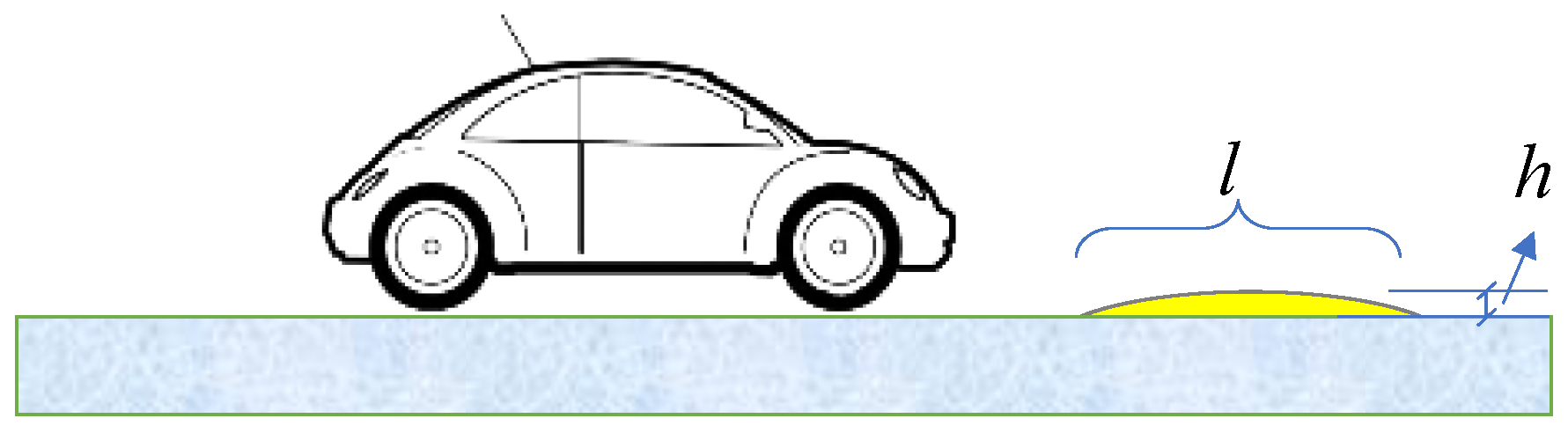
To estimate the FRF $H_{yr}$ of the measured vehicle response with respect to the road roughness, a driving test was designed based on Equation (8) using acceleration sensors to measure the vehicle response $Y\left(\omega \right)$. A known hump is designed using the cosine wave expressed in Equation (18). Let a car drive over the hump with a constant velocity, as shown in Figure 2. The shape of the hump surface represents the displacement of the wheel–road contact point, which in the frequency domain is taken as the road roughness $R\left(\omega \right)$ in Equation (8).

$$r\left(z\right)=\frac{h\left(1-cos\left(\frac{2\pi z}{l}\right)\right)}{2},0\le z\le l$$

(18)

For the half-car model shown in Figure 1, the number of wheel–road contact points is two, and the dimension of the frequency transfer function matrix $H_{yr}\left(\omega \right)$ in Equation (8) is q × 2, where q is the number of sensors located on the vehicle. The dimensions of the contact displacement $R\left(\omega \right)$ are 2 × 1. To accurately estimate the function $H_{yr}\left(\omega \right)$, it is advisable to perform multiple-group tests with different driving speeds to obtain effective data with different frequency bands. Although the shape of the road surface is the same in the tests, the time histories of the contact displacements $r\left(t\right)$ are different owing to different vehicle driving speeds. $r_i\left(t\right)$ and $y_i\left(t\right)$ denote the displacements of the contact points and measured vehicle responses in the ith test, respectively. Accordingly, $R_i\left(\omega \right)$ and $Y_i\left(\omega \right)$ are their Fourier transforms in the frequency domain.

Based on Equation (8), the measured responses $Y_i\left(\omega \right)$ and the corresponding contact displacements $R_i\left(\omega \right)$ from the tests are assembled and expressed in Equation (19). The least-squares method can then be used to estimate the FRF ${\stackrel{-}{H}}_{yr}\left(\omega \right)$ as shown in Equation (20) which represents the relation between the measured vehicle responses and the road roughness.

$$\{\begin{array}{l}\stackrel{-}{Y}\left(\omega \right)={\stackrel{-}{H}}_{yr}\left(\omega \right)\stackrel{-}{R}\left(\omega \right)\\ \stackrel{-}{Y}\left(\omega \right)=\left[Y_1\left(\omega \right),Y_2\left(\omega \right),\cdots ,Y_k\left(\omega \right)\right]\\ \stackrel{-}{R}\left(\omega \right)=\left[R_1\left(\omega \right),R_2\left(\omega \right),\cdots ,R_k\left(\omega \right)\right]\end{array}$$

(19)

$${\stackrel{-}{H}}_{yr}\left(\omega \right)=\stackrel{-}{Y}\left(\omega \right){\stackrel{-}{R}}^T\left(\omega \right)(\stackrel{-}{R}\left(\omega \right){\stackrel{-}{R}}^T\left(\omega \right){)}^{-1}$$

(20)

3.2. Updating the Estimated FRF Based on the Shape Function Method

The direct estimation of the structural FRF using Equation (20) may result in errors due to noise and the frequency band range of the hump excitation. The noise mainly includes test and environmental noises. The frequency band range of the hump excitation depends on the driving velocity, and in the frequency band range corresponding to the excitation with a small amplitude, there will be a relatively large FRF estimation error, which may even cause singular data in those local frequency ranges.

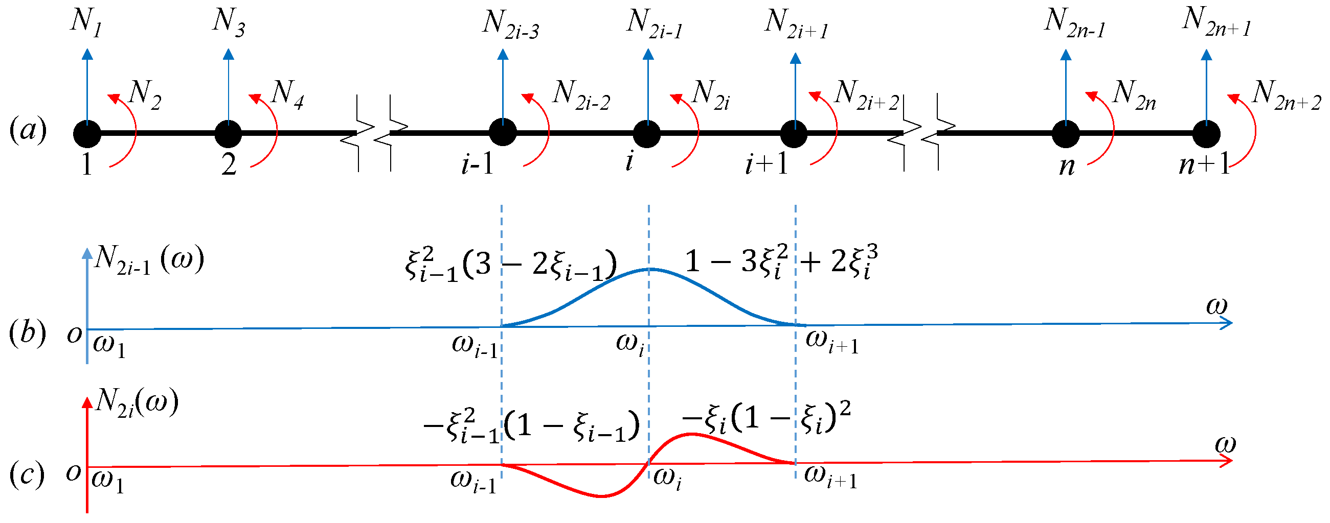
The frequency response is complex and consists of real and imaginary parts. For the FRF of a car, the real and imaginary parts are generally continuous and smooth curves considering vehicle damping. In this way, the shape function method [36] is employed here to fit the real and imaginary parts of the estimated FRF in its local frequency band range with a data singularity to reduce the estimation error. In the shape function method, a continuous curve is compared to the bending deformation of a beam, and the curve is approximated by interpolation. In Figure 3 it can be seen that the curve is divided into several segments. Each segment is considered as a beam element, and the node of each segment is equivalent to the endpoint of the beam element. Using the property of the shape function in the finite element, the value at any point of the curve (the deformation of the beam) can be expressed by the rotation angle and displacement of the node of the segment.

As shown in Figure 3a, the curve is divided into n segments (elements) with a total of n + 1 nodes, and the number of shape functions is 2n + 2. The frequency coordinate corresponding to the ith node is denoted by ${\omega }_i$ as shown in Figure 3b, and N_2i−1(ω) represents the shape function corresponding to its unit vertical deformation, the expression of which is shown in Equation (21). The shape function corresponding to its unit rotational angle is defined as N_2i(ω), the expression of which is shown in Equation (22).

$$\{\begin{array}{c}{N}_{2i-1}\left(\omega \right)=0\omega <{\omega }_{i-1}\mathrm{or}\omega >{\omega }_{i+1}\\ N_{2i-1}\left({\xi }_{i-1}\right)={\xi }_{i-1}^2\left(3-2{\xi }_{i-1}\right);{\xi }_{i-1}=\frac{\omega -{\omega }_{i-1}}{{\omega }_i-{\omega }_{i-1}},{\omega }_{i-1}<\omega <{\omega }_i\\ N_{2i-1}\left({\xi }_i\right)=1-3{\xi }_i^2+2{\xi }_i^3;{\xi }_i=\frac{\omega -{\omega }_i}{{\omega }_{i+1}-{\omega }_i},{\omega }_i<\omega <{\omega }_{i+1}\end{array}$$

(21)

$$\{\begin{array}{c}{N}_{2i}\left(\omega \right)=0;\omega <{\omega }_{i-1}\mathrm{or}\omega >{\omega }_{i+1}\\ N_{2i}\left({\xi }_{i-1}\right)=-{\xi }_{i-1}^2\left(1-{\xi }_{i-1}\right);{\xi }_{i-1}=\frac{\omega -{\omega }_{i-1}}{{\omega }_i-{\omega }_{i-1}},{\omega }_{i-1}<\omega <{\omega }_i\\ N_{2i-1}\left({\xi }_i\right)=-{\xi }_i{\left(1-{\xi }_i\right)}^2;{\xi }_i=\frac{\omega -{\omega }_i}{{\omega }_{i+1}-{\omega }_i},{\omega }_i<\omega <{\omega }_{i+1}\end{array}$$

(22)

Taking the shape functions $N_j\left(\omega \right)$ (j = 1,2,…,2n + 2) as a set of bases, $h\left(\omega \right)$ is assumed to be the real or imaginary part of the frequency response that needs to be updated, and the curve of $h\left(\omega \right)$ can be approximately expressed by these bases and is shown in Equation (23):

$$h\left(\omega \right)={\sum }_{j=1}^{2n+2}{N}_j\left(\omega \right){\alpha }_j,$$

(23)

where ${\alpha }_j$ is the coefficient of the jth shape function. All the directly estimated FRF data $h\left({\omega }_a\right)$ (a = 1,2,…) are assembled into a column vector $h$ that corresponds to the frequency coordinates ${\omega }_a$ (a = 1,2,…), and all the coefficients are assembled into vector $\alpha ={\left[{\alpha }_1,{\alpha }_2,\dots ,{\alpha }_{2n+2}\right]}^{\mathrm{T}}$; then, Equation (23) can be rewritten as a system of linear equations as shown in Equation (24).

$$h=N\alpha ,$$

(24)

where $N$ is a matrix that collects the shape functions $N_j\left({\omega }_a\right)$ (j = 1,2,…,2n + 2; a = 1,2,…). The coefficient $\alpha$ can be calculated by the least-squares method, as shown in Equation (25).

$$\alpha ={\left(N^{\mathrm{T}}N\right)}^{-1}{N}^{\mathrm{T}}h,$$

(25)

The singular data in the directly estimated FRF are certain to cause large errors in the calculation of the coefficient $\alpha$. In this study, singular data are eliminated by setting the threshold value, and an iterative solution is adopted to calculate the coefficient $\alpha$, as expressed in Equation (26):

$${\alpha }^{b+1}={\left(N^{\mathrm{T}}{Q}^{b}N\right)}^{-1}{N}^{\mathrm{T}}{Q}^{b}h,$$

(26)

where ${\alpha }^{b+1}$ is the calculated coefficient in the bth iteration. Herein, the initial value ${\alpha }^1=0$. $Q^b$ represents the weight matrix of the bth iteration, which is a diagonal matrix constituted by the weights $q^b\left({\omega }_a\right)$ (a = 1,2,…). The expression of $q^b\left({\omega }_a\right)$ is given by Equation (27).

$$q^b\left({\omega }_a\right)=\{\begin{array}{c}0,\left|h\left({\omega }_a\right)-{\sum }_{j=1}^{2n+2}{N}_j\left({\omega }_a\right){\alpha }_j^b\right|>{\mathsf{\beta }}^b\\ 1,\left|h\left({\omega }_a\right)-{\sum }_{j=1}^{2n+2}{N}_j\left({\omega }_a\right){\alpha }_j^b\right|\le {\mathsf{\beta }}^b\end{array},$$

(27)

where ${\mathsf{\beta }}^b$ is the threshold for judging whether or not the data are singular. With an increase in iterations, the threshold ${\mathsf{\beta }}^b$ decreases. The iteration stops when the function converges. By substituting the coefficient ${\alpha }^{b+1}$ from the last iteration into Equation (24), the singular data in the frequency response curve can be eliminated. Then, using the obtained vehicle FRF, the road roughness can be estimated by Equation (16) using the measured vehicle responses.

3.3. On-Line Estimation of Road Roughness

Via the vehicle FRF calibrated in advance, the road roughness can be estimated using the measured vehicle responses. The process is performed in the frequency domain, which generally requires the responses to be measured in a certain time period to perform Fourier transform and the estimation. In this case, the following method of segmented data acquisition and calculation is proposed in this paper to achieve on-line identification of road roughness:

(1) Denote by T the time interval for on-line estimation. For the ith time period t ∈$\left(t_i,t_i+4T\right)$, $t_i=\left(i-1\right)T$, the responses measured in the time period t ∈ $\left(t_i,t_i+4T\right)$ are used for road roughness estimation, defined as ${\widehat{r}}_i\left(t\right)$, t ∈ $\left(t_i,t_i+4T\right)$.

(2) Since the initial state of the vehicle is usually unknown, estimation errors can appear in the initial time period. Considering the time coincidence between the ith and the (i − 1)th estimation periods, the estimation accuracy can be improved by combining the two estimated roughness profiles in the overlapping time period. Therefore, the on-line road roughness estimation is performed as shown in Equation (28)

$$\{\begin{array}{l}r\left(t\right)=\left(\frac{t_i+2T-t}{T}\right){\widehat{r}}_{i-1}\left(t\right)+\left(\frac{t-t_i-T}{T}\right){\widehat{r}}_i\left(t\right)\mathrm{for}t\in \left(t_i+T,t_i+2T\right),\\ r\left(t\right)={\widehat{r}}_i\left(t\right)\mathrm{for}t\in \left(t_i+2T,t_i+4T\right),\end{array}$$

(28)

where $\left(\frac{t_i+2T-t}{T}\right)$ and $\left(\frac{t-t_i-T}{T}\right)$ are the weighting coefficients of the two overlapping time periods in order to make the estimated road roughness curve continuous.

(3) Let i = i + 1, and repeat the above steps.

4. Numerical Simulation

To numerically demonstrate the proposed methods, a half-car model with four DOFs is used. The vehicle model parameters are listed in

Table 1. Parameters values of the vehicle model.

m1 (kg)	m2 (kg·m2)	m3 (kg)	m4 (kg)	k1 = k2 (N/m)	k3 = k4 (N/m)	c1 = c2 (N·s /m)	e1 (m)	e2 (m)
1000	4000	100	150	20,000	300,000	4000	1.6	1.6

, which are selected based on reference [11].

4.1. Characteristic Analysis of the Vehicle FRF

The four natural frequencies are shown in

Table 2. Four natural frequencies of the half-car model (Hz).

Order	1	2	3	4
natural frequency	0.779	0.974	7.355	9.006

and correspond to the bouncing, pitching, front axle, and rear axle-top modes of the vehicle.

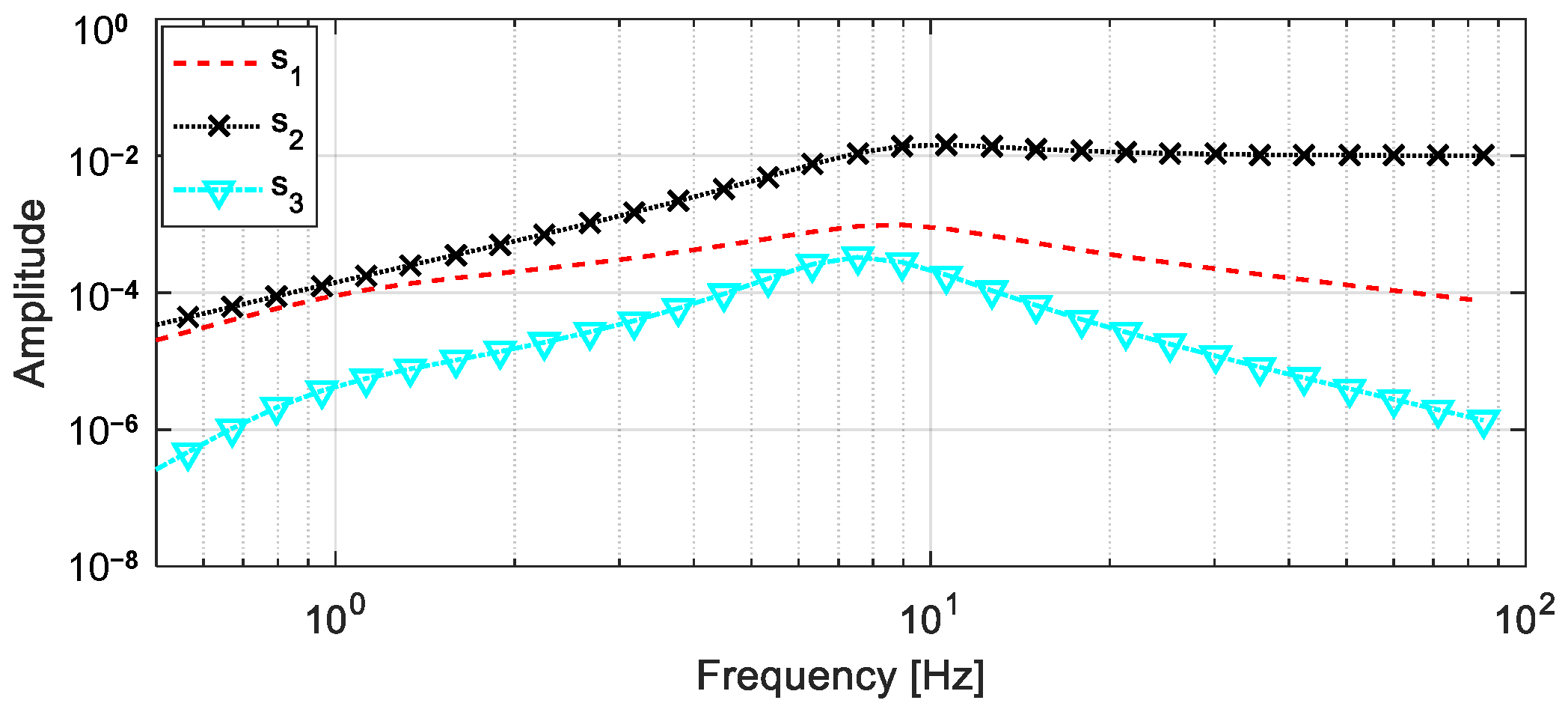
Vehicle accelerations, which are generally easy to obtain via sensors, were measured in this study. It was assumed that three sensors were located along the DOFs of the vehicle body u₁, rear wheel u₃, and front wheel u₄, denoted by S₁, S₂, and S₃, respectively. The vehicle vertical acceleration responses are measured, and the observation matrix C₀ is shown in Equation (29).

$$C_0=\left[\begin{array}{cccc}1& 0& 0& 0\\ 0& 0& 1& 0\\ 0& 0& 0& 1\end{array}\right]$$

(29)

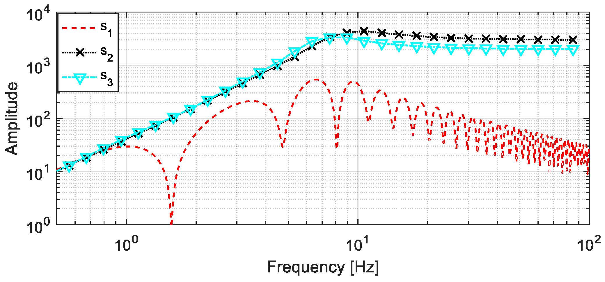
By applying a unit impulse on the rear wheel along DOF u₃, the acceleration frequency responses of the vehicle at the measurement points can be expressed as $H_{su}\left(\omega \right)=-{\omega }^2{C}_0{H}_{uu}\left(\omega \right)B_{u3}$, where $B_{u3}={\left[\begin{array}{cccc}0& 0& 1& 0\end{array}\right]}^{\mathrm{T}}$, and the amplitude of the corresponding frequency responses are shown in Figure 4. Taking the unit vertical displacement of the rear wheel contact point, that is, the road roughness, as the excitation, the observed acceleration frequency responses of the vehicle can be expressed as $H_{sr}\left(\omega \right)=-{\omega }^2{C}_0{H}_{ur}\left(\omega \right)B_{r1}$, where $B_{r1}={\left[\begin{array}{cc}1& 0\end{array}\right]}^{\mathrm{T}}$. Their amplitudes are shown in Figure 5. Although the amplitudes of the two types of frequency responses shown in Figure 4 and Figure 5 are different, they have similar change regularities. Comparatively speaking, in the calculation of responses $H_{sr}\left(\omega \right)$, the stiffness and damping of the vehicle wheel are added; therefore, their amplitude is larger than the frequency responses $H_{su}\left(\omega \right)$.

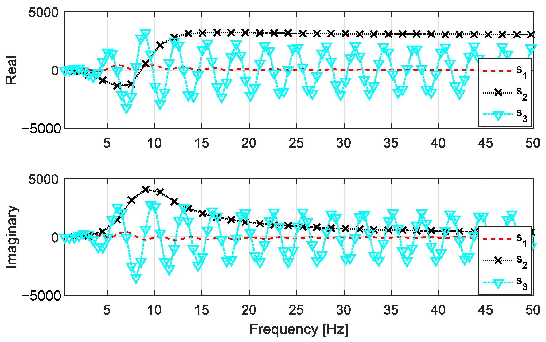
The distance between the front and rear wheels is 3.2 m; therefore, with a driving velocity of 10 m/s, the time shift between the front and rear wheels is t₀ = 0.32 s. Assuming that the front and rear wheels drive along a straight line, the measured acceleration frequency responses of the vehicle with regard to the unit displacement of the rear wheel contact point $H_{yr1}\left(\omega ,v\right)$ can be calculated using Equation (15). Figure 6 shows the amplitude of $H_{yr1}\left(\omega ,v\right)$, and its real and imaginary parts are shown in Figure 7. Because both the front and rear wheels are excited in order, the frequency responses of the vehicle with respect to the rear wheel in Figure 6 and Figure 7 are different from those shown in Figure 4 and Figure 5. There exists a time shift of t₀ = 0.32 s between the excitations applied successively on the front and rear wheels, and there is one more item $e^{j\omega t_0}$ in the corresponding frequency responses; therefore, the frequency response curve has a periodic change rule, i.e., 1/t₀ = 3.12 Hz, which can be seen as “S₃” in Figure 7. It can be seen that there is a phase difference of π/2 between the real and imaginary parts of the acceleration frequency responses of the vehicle.

4.2. Simulation of the Measured Vehicle Accelerations

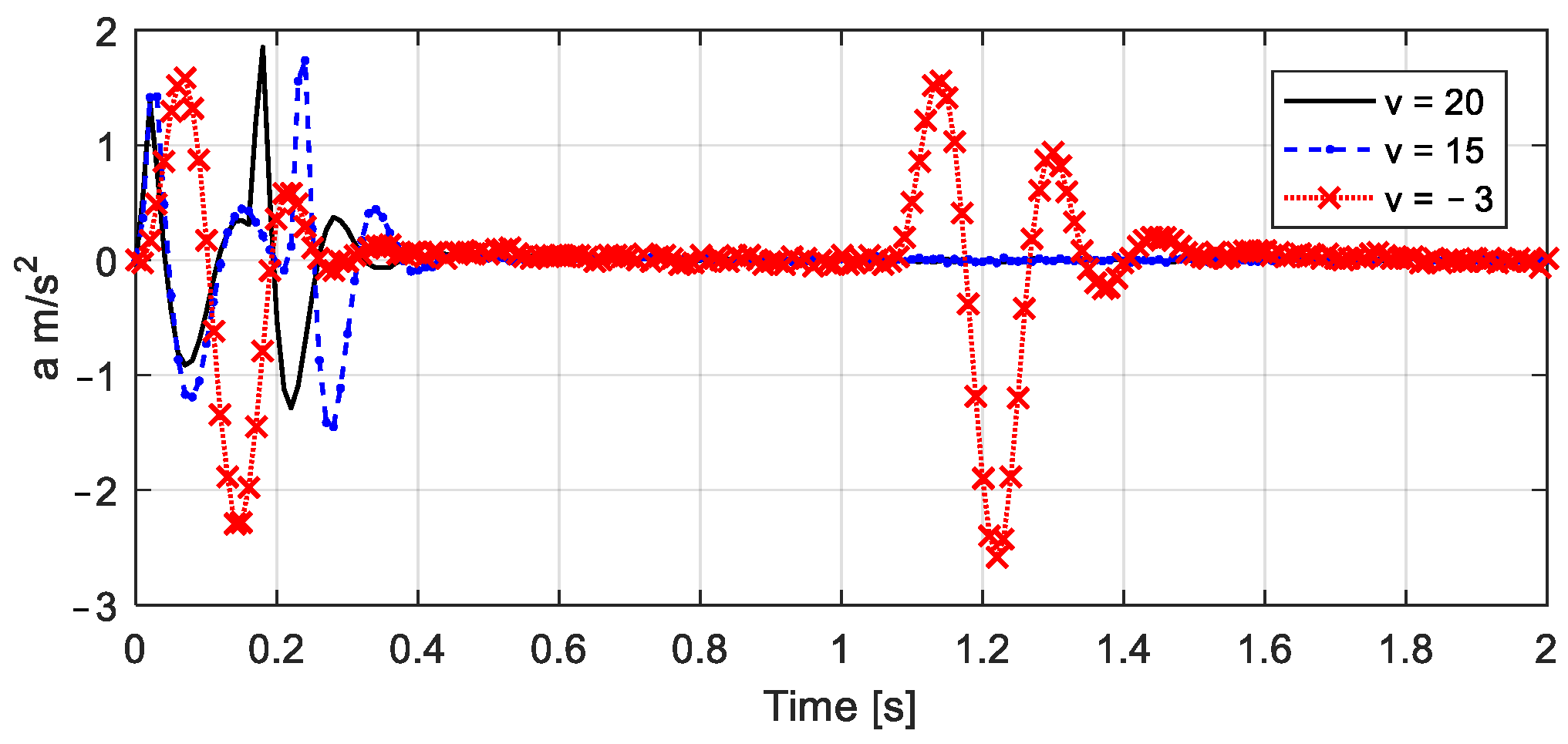
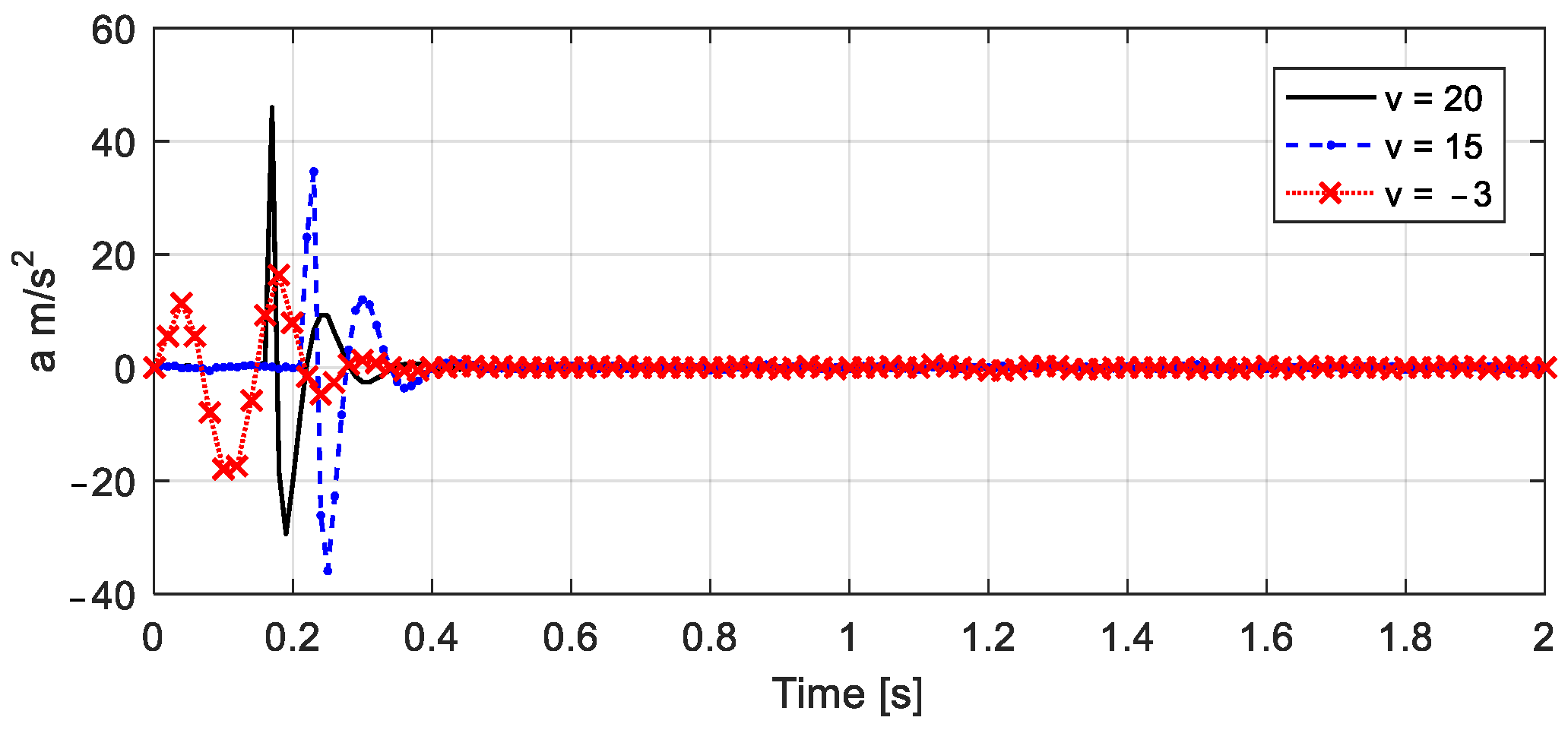
Let the vehicle drive past a well-designed hump shown in Figure 2 with a height h = 0.02 m and length l = 0.5 m. Eight groups of driving tests were performed with velocities of [20, 17, 15, 13, 11, 7, 5, −3] m/s, where a negative value indicates that the car moves backward. In practice, the initial position of the vehicle needs to be at a certain distance from the hump in order to allow the vehicle to accelerate and then run at a constant speed, but in the numerical example, the initial position can be right in front of the hump and the influence of the vehicle wheel shape is also neglected. The measured vehicle accelerations are simulated via the equation of motion of the vehicle, i.e., Equation (1), using the Newmark-β method. Additionally, a 5% Gaussian noise is considered. Figure 8 shows the accelerations of the vehicle body measured by S₁ with velocities of [20, 15, −3] m/s, while Figure 9 shows the accelerations of the rear wheel measured by S₂ with velocities of [20, 15, −3] m/s.

4.3. Estimation of Vehicle FRF

To identify the road roughness via Equations (16) and (17), the vehicle FRF estimation is first discussed and verified using the direct estimation. Furthermore, the shape function method is used to deal with singular points.

4.3.1. Direct Estimation Using Measured Responses

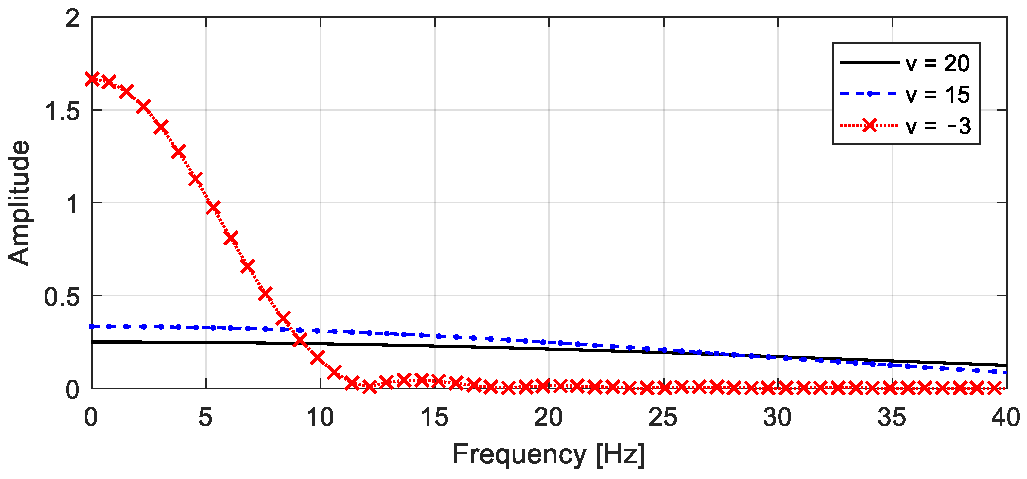
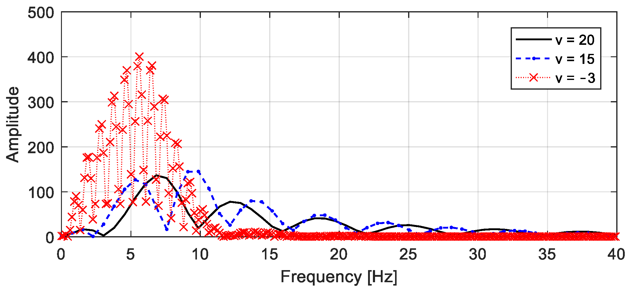
Although the hump profile is the same in the different tests, the time histories of the hump profile, that is, the road roughness, differ with respect to the different driving velocities. The frequency spectra of the hump with respect to different velocities are shown in Figure 10, and the frequency spectra of the vehicle accelerations along DOF u₁ are shown in Figure 11.

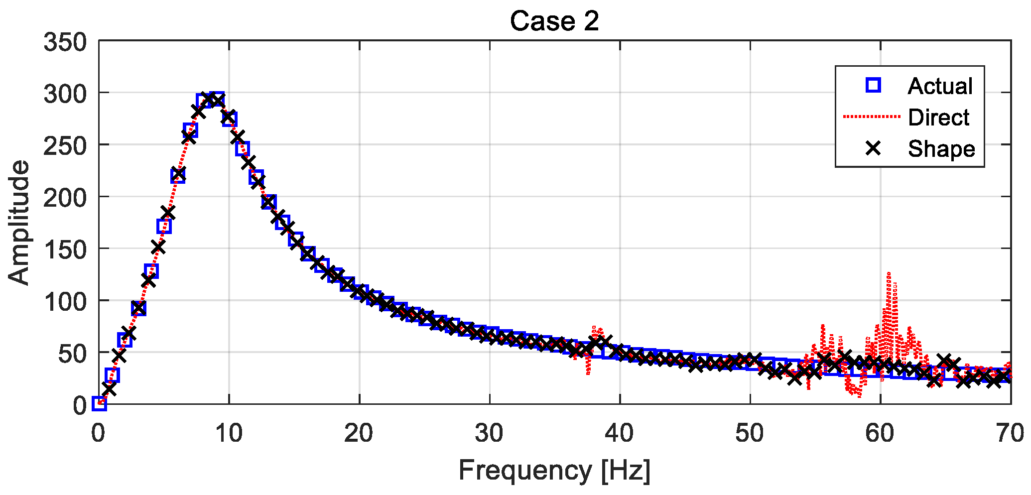
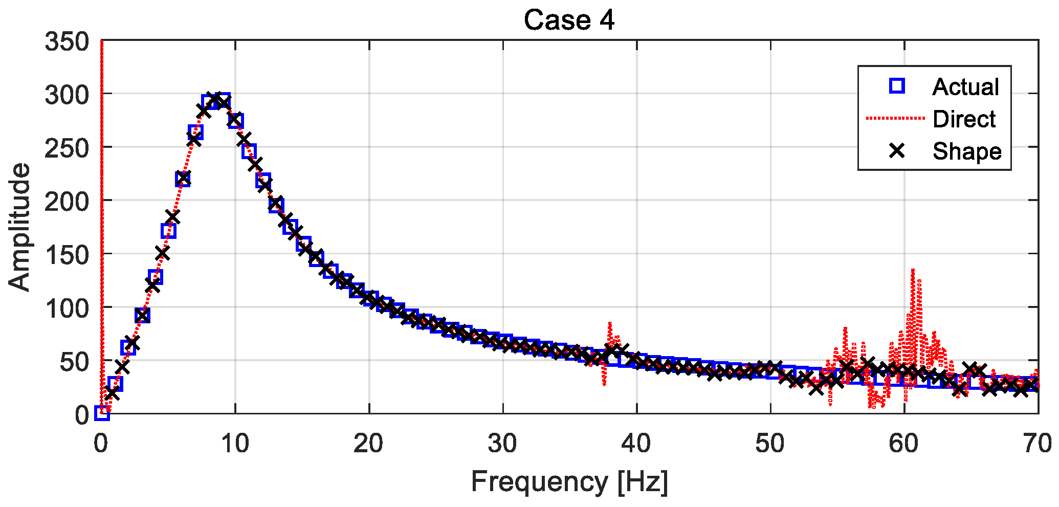
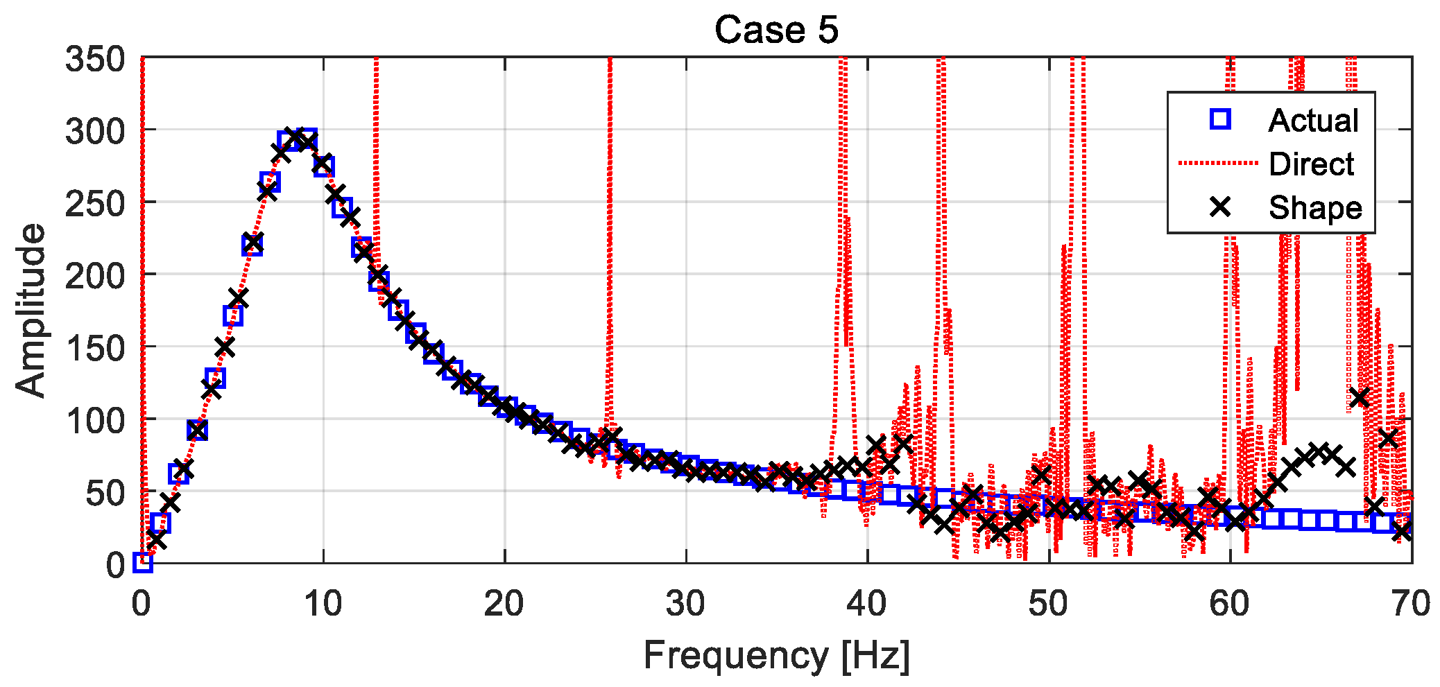
To investigate the influence of the measured data on the FRF estimation, the measured responses were combined into five cases, as shown in

Table 3. Combination of measured responses in different cases.

Case	Case 1	Case 2	Case 3	Case 4	Case 5
Sets of velocity (m/s)	20, 17, 15, 13, 11, 7, 5, −3	20, 15, 11, 5, −3	20, 15, 11, 5	20,15, 1	15, 11

which were employed to estimate the vehicle FRF. In different cases, the amplitudes of the vehicle acceleration FRF along DOF u₁ are estimated and compared in Figure 12, Figure 13, Figure 14, Figure 15 and Figure 16 and denoted as “Direct”. It can be seen that the accuracy is the highest in Case 1 which uses all the measured responses at different speeds. It also shows that the driving speed and measured data volume may influence the estimation results.

It can be seen that the estimated FRF in Case 1 using eight groups of measured data is smoother than those estimated in the remaining cases, and singular data appear in the frequency band range greater than 50 Hz. In Case 2, which uses five groups of measured data, singular data in the FRF appeared around the frequency band range between 19 Hz and 38 Hz and greater than 50 Hz. More singular data appear in Cases 3 and 4, and there is a large quantity of singular data in Case 5. It is worth noting that the estimation error is obvious in the frequency band range larger than 40 Hz because the excitations in that range are close to zero. However, this part of the FRF has little influence on related problems. For brevity, only the related FRFs of the vehicle acceleration along DOF u₁ are shown in this paper, and the estimated FRFs of the rear and front wheels have similar accuracy.

4.3.2. Updating the Vehicle FRF

The vehicle FRF curve is divided into 80 segments, to which the imaginary and real parts are fitted locally via Equation (24), so as to reduce the FRF estimation error. The maximum value of the imaginary or real part is taken as the initial threshold value, and the threshold value is halved in the next iteration. A smooth frequency response curve can be obtained in four iterations.

For the five cases listed in Table 3, the amplitudes of the updated FRFs of the vehicle along DOF u₁ are shown in Figure 12, Figure 13, Figure 14, Figure 15 and Figure 16 and denoted as “Shape.” It can be seen that the influence of data singularities on FRF estimation can be effectively reduced by the shape function method, and even in Case 5, which has serious data singularities, the updated estimation is acceptable. As a result, the robustness of the method to noise and measured data is improved, which provides the advantage of a road roughness estimation.

4.4. Road Roughness Estimation

4.4.1. Road Roughness and Vehicle Response

Currently, the trigonometric series method, which uses a special triangular series to approximate the road surface irregularity curve, is commonly used for road roughness calculations. The expression for the road roughness $r\left(x\right)$ is as follows:

$$r\left(x\right)={\sum }_{k=1}^{N_T}{\alpha }_k\cos \left(2\pi n_{k}x+{\phi }_k\right)$$

(30)

$${\alpha }_k^2=4G_d\left(n_k\right)\Delta n,\Delta n=\frac{n_u-n_l}{N_T},$$

(31)

$$G_d\left(n_k\right)=G_d\left(n_0\right){\left(\frac{n_k}{n_0}\right)}^{-2},n_k=n_l+k\Delta n,$$

(32)

where ${\alpha }_k$ is the coefficient of the triangular series, depending on the roughness degree of the pavement. $G_d\left(n_k\right)$ is the displacement power spectral density of the pavement calculated using the equation provided in [37]. $G_d\left(n_0\right)$ is defined as the coefficient of unevenness and depends on the degree of roughness of the pavement. $n_0$ is the reference special frequency ($n_0=0.1$ circle/m), and $n_k$ is the special frequency. $n_l$ and $n_u$ are the lower and upper limits of the spatial frequency used to calculate the displacement power spectral density $G_d\left(n_k\right)$. ${\phi }_k$ is a uniformly distributed random phase angle in the range of [0 2π]. N_T is the number of trigonometric functions used to construct the road roughness.

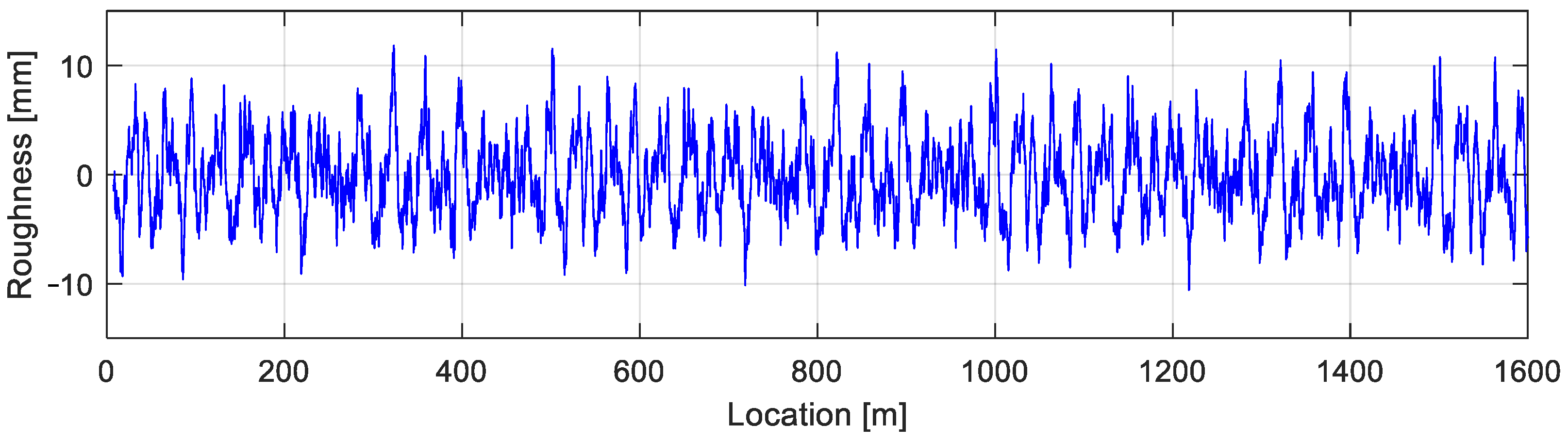
In this study, the road surface grade was set to A, for which the irregularity coefficient $G_d\left(n_0\right)$ was $16\times {10}^{-6}{\mathrm{m}}^3$, $n_l=0.0221{\mathrm{m}}^{-1}$, and $n_u=1.4142{\mathrm{m}}^{-1}$. The considered length of the road surface was 1600 m. The vehicle drove on the road with a velocity of 10 m/s, and the corresponding road roughness is shown in Figure 17.

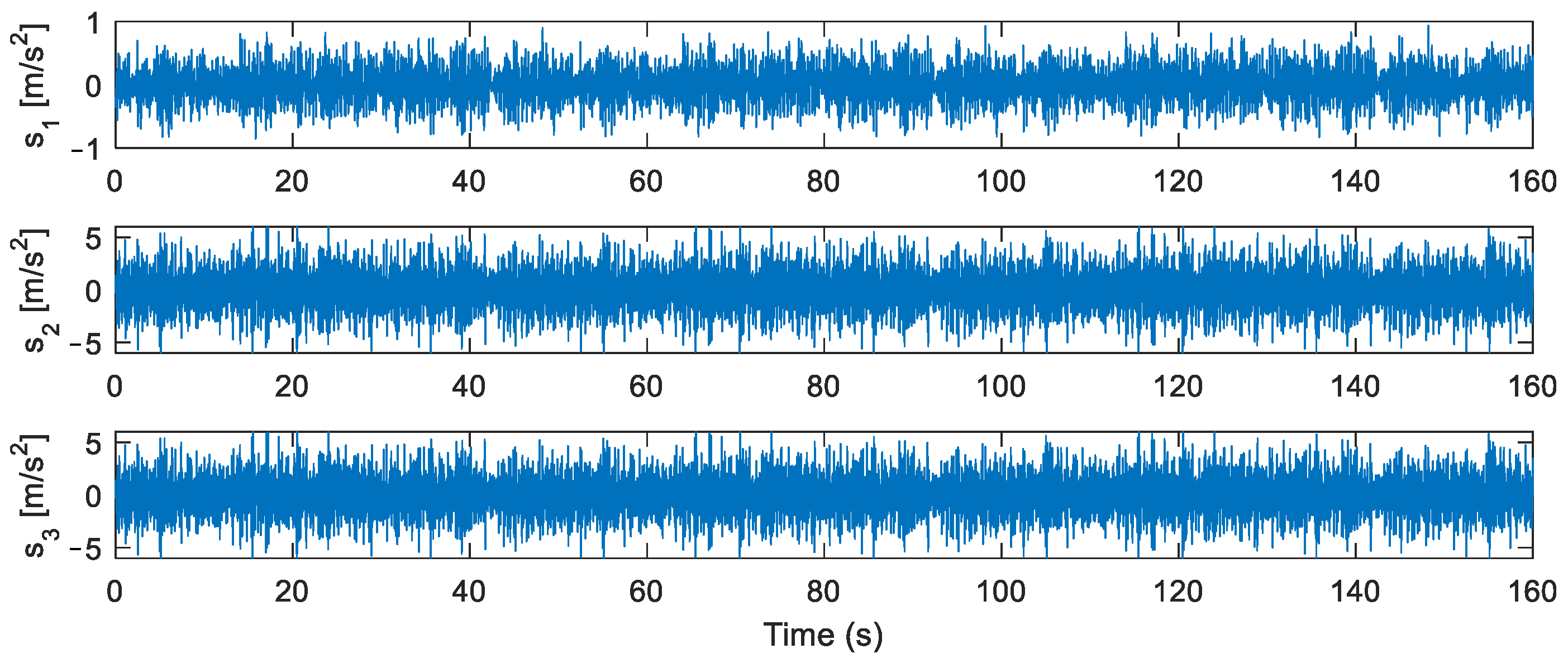
Three acceleration sensors are located on the vehicle: S₁ measures the vertical acceleration response of the vehicle body along DOF u₁, S₂ measures the rear wheel acceleration response along DOF u₂, and S₃ measures the front wheel acceleration response along DOF u₃. The sampling frequency was 400 Hz. The time histories of the measured acceleration responses are shown in Figure 18.

4.4.2. Different Case Estimations

To check the influence of the measured responses, four cases are considered in the road roughness estimation and are listed as follows:

Case A: Estimation is performed using the responses measured by all the sensors, that is, S₁, S₂, and S₃.

Case B: Estimation is performed using the responses measured by sensors S₁ and S₃.

Case C: Estimation is performed using the responses measured by sensors S₁ and S₂.

Case D: Estimation is performed using the responses measured by sensor S₁.

In each case, the frequency spectrum of road roughness $R_1\left(\omega \right)$ was calculated via Equation (11) for the estimated vehicle.

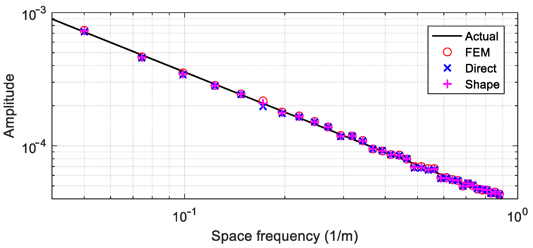
First, the estimation for Case A is taken as an example to validate the proposed method. The vehicle FRF is estimated using the eight groups of measured responses in Case 1 listed in Table 3, and the estimated frequency spectra of road roughness $R_1\left(\omega \right)$ are shown in Figure 19, where “Actual” refers to the actual road roughness. “Direct” refers to the results estimated using the vehicle FRF by the direct method, while “Shape” refers to the results estimated using the vehicle FRF updated by the shape function method, and “FEM” refers to the results estimated using the vehicle FRF computed with the actual vehicle parameters. To compare the estimation accuracy, Figure 20 shows the corresponding absolute errors of the estimated road roughness, which refers to the difference between the estimated road roughness and the actual road roughness. It can be seen that the errors are quite small, which proves that the road roughness is estimated accurately using the above methods. The power spectral densities of the estimated road roughness are computed and shown in Figure 21 and are almost identical to the actual values.

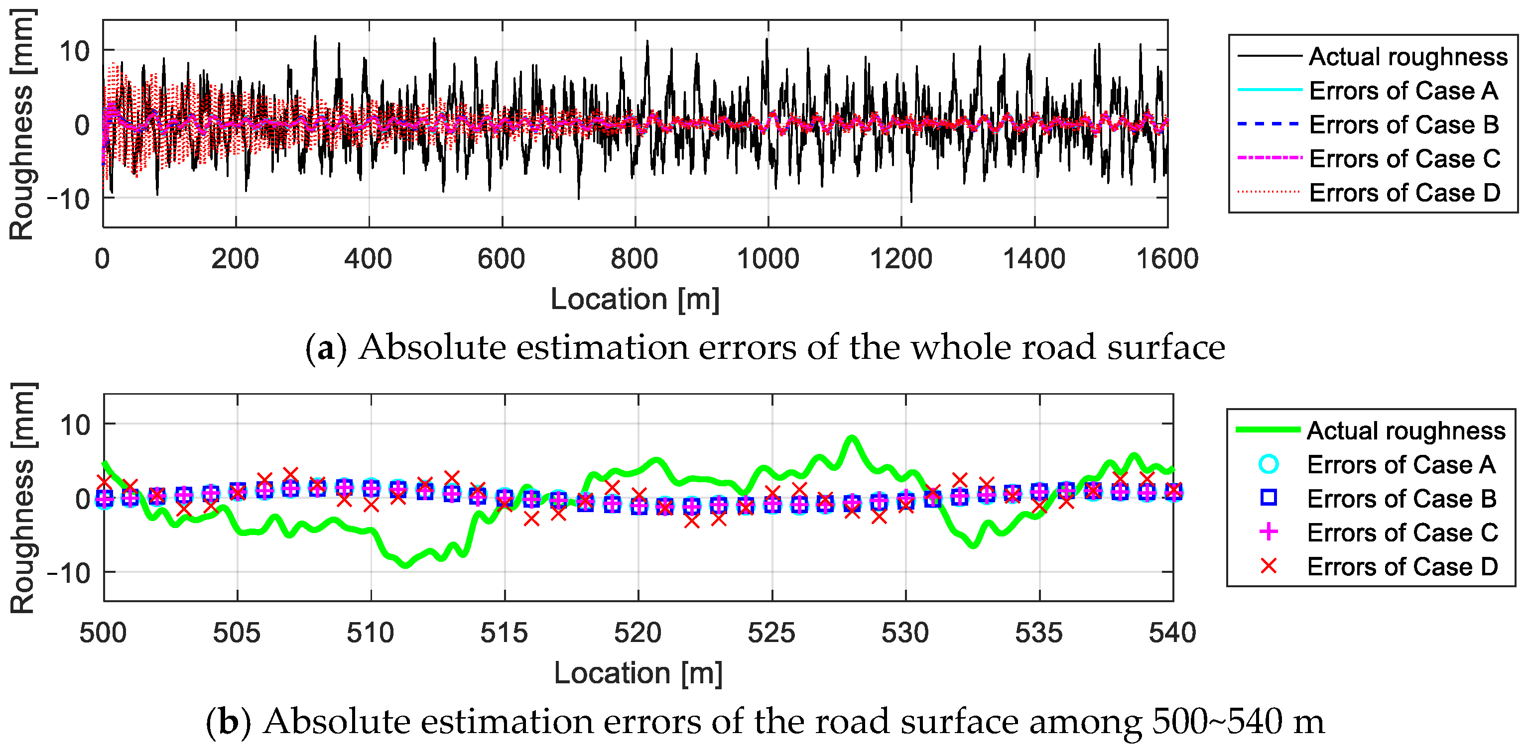
In Cases A–D, the road roughness is estimated via the vehicle FRF using direct estimation and the updated method. The corresponding absolute errors are shown respectively in Figure 22 and Figure 23. It can be seen that the estimation accuracy is good in Cases A–C, which have at least two sensors, while in Case D with only one sensor, the error is quite large.

4.4.3. Error Analysis

Considering that the vehicle FRF is estimated using the test of driving over the hump in Cases 1–5, which are listed in Table 3, the road roughness is estimated using the sensors shown in Cases A–D to analyze the influence of the frequency response estimation and the sensors. The estimation errors here are quantitatively calculated using Equation (33) in terms of the relative error:

$$\epsilon =\Vert r_{id}\left(t\right)-r\left(t\right)\Vert /\Vert r\left(t\right),$$

(33)

where r_id(t) refers to the estimated road roughness, and r(t) refers to the actual road roughness. The errors corresponding to the direct FRF estimation, the updated FRF, and the FRF obtained via the FEM are shown in

Table 4. Errors of the estimated road roughness using the directly estimated FRF.

	Case A	Case B	Case C	Case D
Case 1	17.02%	16.82%	16.07%	31.10%
Case 2	24.67%	22.67%	20.17%	47.71%
Case 3	23.21%	23.16%	16.73%	38.03%
Case 4	54.33%	35.60%	53.53%	48.09%
Case 5	54.85%	42.51%	53.49%	52.85%

,

Table 5. Errors of the estimated road roughness using the updated FRF.

	Case A	Case B	Case C	Case D
Case 1	10.26%	10.43%	10.50%	28.76%
Case 2	11.67%	11.63%	11.57%	45.66%
Case 3	15.29%	12.68%	13.72%	33.36%
Case 4	59.89%	41.05%	57.57%	36.70%
Case 5	61.70%	46.58%	60.14%	42.95%

and

Table 6. Errors of the estimated road roughness using the FRF of the FEM.

	Case A	Case B	Case C	Case D
Errors	8.55%	8.75%	8.88%	16.39%

. In case D, where only one sensor S₁ is employed, the estimation errors are about 30% even with the accurate estimated vehicle FRF in Case 1. On the other hand, the estimation errors in Case 4 and Case 5 are also quite high, which means that the poor estimation of vehicle FRF definitely influences the road roughness estimation even with all the three sensors used in Case A.

By observing the errors listed in Table 4, Table 5 and Table 6, the following conclusions can be drawn:

(1) Owing to the noise influence, the error still exists, approximately 8% in Cases A–C, even when using the FRF obtained by the vehicle FEM. The shape function method can improve the estimation accuracy of the vehicle FRF, and correspondingly, the estimation accuracy of the road roughness is increased using the updated FRF, which is approximately 10% in Case 1 and Cases A–C in Table 5.

(2) The more groups of driving tests with different speeds over a hump are performed, the more accurate the estimated frequency response is. Good results can be obtained by using the four groups of the driving tests shown in Case 3 and Cases A–C in Table 5.

(3) The location of two or three sensors in Cases A–C can provide a more accurate road roughness estimation, while the result via sensor S₁ in case D is relatively poor.

4.4.4. On-Line Estimation of Road Roughness

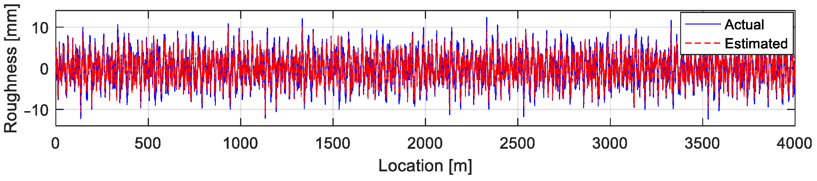
In this work, the road surface grade was set to A as mentioned in Section 4.4.1. The considered length of the road surface was 4000 m. The vehicle drove on the road with a velocity of 10 m/s, and the corresponding road roughness is shown in Figure 24.

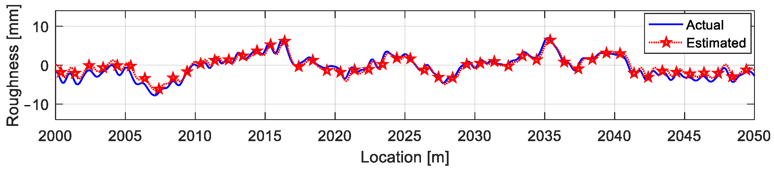
Three acceleration sensors are employed with the same placements as those in Case A in Section 4.4.2. The sampling frequency was 400 Hz. The road roughness estimation is performed on-line with a time interval of 2.56 s. Assume that the vehicle runs for 400 s, and therefore it requires 154 times of on-line estimation step by step as described in Equation (28). The time histories of the estimated roughness of the whole road surface are shown in Figure 24 and Figure 25 show the estimated results of the road surface between 2000 and 2050 m. It can be seen that the estimation accuracy is good.

5. Conclusions

A road roughness estimation method is proposed in the frequency domain based on the vehicle FRF via the measured vehicle accelerations. A numerical simulation of the road roughness estimation was used to verify the effectiveness of the proposed methods. The main conclusions are as follows:

The formula for the vehicle response, road roughness, and vehicle FRF is deduced and set up in a linear equation system; hence, the road roughness can be estimated using the vehicle FRF and the measured vehicle responses.

The vehicle FRF is estimated by designing multiple groups of driving tests over a known-size hump at different driving speeds. It obviates the need for an updated finite element model of the vehicle with known vehicle parameters and vehicle modeling.

The vehicle FRF can be calculated by a direct estimation of the measured vehicle accelerations using the least-squares method. Moreover, the shape function method can be used to eliminate the singular and noisy parts of the estimated FRF and to improve the accuracy of the estimated road roughness profile. The road roughness can be estimated online with a few seconds time delay.

References

- Ihs, A. The influence of road surface condition on traffic safety and ride comfort. In Proceedings of the 6th International Conference on Managing Pavements, Brisbane, Australian, 19–24 October 2004. [Google Scholar]
- Hanafi, D.; Huq, M.S.; Suid, M.S.; Rahmat, M. A Quarter Car ARX Model Identification Based on Real Car Test Data. J. Telecommun. Electron. Comput. Eng. 2017, 9, 135–138. [Google Scholar]
- Otremba, F.; Navarrete, J.A.R.; Guzmán, A.A.L. Modelling of a partially loaded road tanker during a braking-in-a-turn maneuver. Actuators 2018, 7, 45. [Google Scholar] [CrossRef] [Green Version]
- Qinghua, M.; Huifeng, Z.; Fengjun, L. Fatigue failure fault prediction of truck rear axle housing excited by random road roughness. Int. J. Phys. Sci. 2011, 6, 1563–1568. [Google Scholar] [CrossRef]
- Reza-Kashyzadeh, K.; Ostad-Ahmad-Ghorabi, M.J.; Arghavan, A. Investigating the effect of road roughness on automotive component. Eng. Fail. Anal. 2014, 41, 96–107. [Google Scholar] [CrossRef]
- Shi, J.; Gao, Y.; Long, X.; Wang, Y. Optimizing rail profiles to improve metro vehicle-rail dynamic performance considering worn wheel profiles and curved tracks. Struct. Multidiscip. Optim. 2021, 63, 419–438. [Google Scholar] [CrossRef]
- Ngwangwa, H.M. Calculation of road profiles by reversing the solution of the vertical ride dynamics forward problem. Cogent Eng. 2020, 7, 1833819. [Google Scholar] [CrossRef]
- Yang, Y.; Cheng, Q.; Zhu, Y.; Wang, L.; Jin, R. Feasibility study of tractor-test vehicle technique for practical structural condition assessment of beam-like bridge deck. Remote Sens. 2020, 12, 114. [Google Scholar] [CrossRef] [Green Version]
- Burger, M. Calculating road input data for vehicle simulation. Multibody Syst. Dyn. 2014, 31, 93–110. [Google Scholar] [CrossRef]
- Kumar, P.; Lewis, P.; Mcelhinney, C.P.; Rahman, A.A. An algorithm for automated estimation of road roughness from mobile laser scanning data. Photogramm. Rec. 2015, 30, 30–45. [Google Scholar] [CrossRef] [Green Version]
- Zhao, B.; Nagayama, T.; Xue, K. Road profile estimation, and its numerical and experimental validation, by smartphone measurement of the dynamic responses of an ordinary vehicle. J. Sound Vib. 2019, 457, 92–117. [Google Scholar] [CrossRef]
- Zhang, Q.; Jankowski, Ł.; Duan, Z. Identification of coexistent load and damage. Struct. Multidiscip. Optim. 2010, 41, 243–253. [Google Scholar] [CrossRef]
- Xu, Z.D.; Huang, X.H.; Xu, F.H.; Yuan, J. Parameters optimization of vibration isolation and mitigation system for precision platforms using non-dominated sorting genetic algorithm. Mech. Syst. Signal Process. 2019, 128, 191–201. [Google Scholar] [CrossRef]
- Guo, S.S.; Shi, Q. Transient influence of correlation between excitations on system responses. Commun. Nonlinear Sci. Numer. Simul. 2020, 80. [Google Scholar] [CrossRef]
- Imine, H.; Delanne, Y.; M’Sirdi, N.K. Road profile input estimation in vehicle dynamics simulation. Veh. Syst. Dyn. 2006, 44, 285–303. [Google Scholar] [CrossRef]
- Ngwangwa, H.M.; Heyns, P.S.; Labuschagne, F.J.J.; Kululanga, G.K. Reconstruction of road defects and road roughness classification using vehicle responses with artificial neural networks simulation. J. Terramech. 2010, 47, 97–111. [Google Scholar] [CrossRef] [Green Version]
- Doumiati, M.; Victorino, A.; Charara, A.; Lechner, D. Estimation of road profile for vehicle dynamics motion: Experimental validation. In Proceedings of the 2011 American Control Conference, San Francisco, CA, USA, 29 June–1 July 2011. [Google Scholar]
- Fauriat, W.; Mattrand, C.; Gayton, N.; Beakou, A.; Cembrzynski, T. Estimation of road profile variability from measured vehicle responses. Veh. Syst. Dyn. 2016, 54, 585–605. [Google Scholar] [CrossRef]
- Kang, S.W.; Kim, J.S.; Kim, G.W. Road roughness estimation based on discrete Kalman filter with unknown input. Veh. Syst. Dyn. 2019, 57, 1530–1544. [Google Scholar] [CrossRef]
- Kim, G.W.; Kang, S.W.; Kim, J.S.; Oh, J.S. Simultaneous estimation of state and unknown road roughness input for vehicle suspension control system based on discrete Kalman filter. Proc. Inst. Mech. Eng. Part D J. Automob. Eng. 2020, 234, 1610–1622. [Google Scholar] [CrossRef]
- Jiang, J.; Seaid, M.; Mohamed, M.S.; Li, H. Inverse algorithm for real-time road roughness estimation for autonomous vehicles. Arch. Appl. Mech. 2020, 90, 1333–1348. [Google Scholar] [CrossRef]
- Jeong, J.H.; Jo, H.; Ditzler, G. Convolutional neural networks for pavement roughness assessment using calibration-free vehicle dynamics. Comput. Civ. Infrastruct. Eng. 2020, 35, 1209–1229. [Google Scholar] [CrossRef]
- Bhowmik, B.; Tripura, T.; Hazra, B.; Pakrashi, V. First-Order Eigen-Perturbation Techniques for Real-Time Damage Detection of Vibrating Systems: Theory and Applications. Appl. Mech. Rev. 2019, 71. [Google Scholar] [CrossRef]
- Panda, S.; Tripura, T.; Hazra, B. First-Order Error-Adapted Eigen Perturbation for Real-Time Modal Identification of Vibrating Structures. J. Vib. Acoust. Trans. ASME 2021, 143. [Google Scholar] [CrossRef]
- Andrén, P. Power spectral density approximations of longitudinal road profiles. Int. J. Veh. Des. 2006, 40, 2–14. [Google Scholar] [CrossRef]
- Liu, X.; Wang, H.; Shan, Y.; He, T. Construction of road roughness in left and right wheel paths based on PSD and coherence function. Mech. Syst. Signal Process. 2015, 60, 668–677. [Google Scholar] [CrossRef]
- González, A.; O’Brien, E.J.; Li, Y.Y.; Cashell, K. The use of vehicle acceleration measurements to estimate road roughness. Veh. Syst. Dyn. 2008, 46, 483–499. [Google Scholar] [CrossRef]
- Qin, Y.; Guan, J.; Gu, L. The research of road profile estimation based on acceleration measurement. Appl. Mech. Mater. 2012, 226–228, 1614–1617. [Google Scholar] [CrossRef]
- Akcay, H.; Turkay, S. Cramer-Rao bounds for road profile estimation. In Proceedings of the 2017 IEEE 3rd Colombian Conference on Automatic Control (CCAC), Cartagena, Colombia, 18 October 2017. [Google Scholar]
- Türkay, S.; Akçay, H. Modelling of road roughness for full-car models: A spectral factorization approach. In Proceedings of the 20th International Conference on System Theory, Control and Computing (ICSTCC), Sinaia, Romania, 13–15 October 2016. [Google Scholar]
- Turkay, S.; Akcay, H. Road roughness modelling by using spectral factorization methods. In Proceedings of the 2016 16th International Conference on Control, Automation and Systems (ICCAS), Gyeongju, Korea, 16–19 October 2016. [Google Scholar]
- Zhao, B.; Nagayama, T. IRI Estimation by the Frequency Domain Analysis of Vehicle Dynamic Responses. Procedia Eng. 2017, 188, 9–16. [Google Scholar] [CrossRef]
- Zhao, B.; Nagayama, T.; Toyoda, M.; Makihata, N.; Takahashi, M.; Ieiri, M. Vehicle model calibration in the frequency domain and its application to large-scale IRI estimation. J. Disaster Res. 2017, 12, 446–455. [Google Scholar] [CrossRef]
- Hansen, P.C. Rank-Deficient and Discrete Ill-Posed Problems: Numerical Aspects of Linear Inversion; SIAM: Philadelphia, PA, USA, 1998; pp. 175–206. [Google Scholar]
- Pan, C.D.; Yu, L.; Liu, H.L. Identification of moving vehicle forces on bridge structures via moving average Tikhonov regularization. Smart Mater. Struct. 2017, 26, 085041. [Google Scholar] [CrossRef]
- Zhang, Q.; Dduan, Z.; Jankowski, Ł. Experimental validation of a fast dynamic load identification method based on load shape function. J. Vib. Shock 2011, 9, 98–102. [Google Scholar] [CrossRef]
- GB/T7031-2005/ISO 8608. Mechanical Vibration-Road Surface Profiles-Reporting of Measured Data of National Standard of the People’s Republic of China; International Organization for Standardization: Geneva, Switzerland, 1995. [Google Scholar]
Figure 1.
Half-car model of the vehicle.
Figure 2.
Diagram of a car driving over a hump.
Figure 3.
Basic principle of the shape function method. (a) Division of the curve; (b) The shape function corresponding to the unit vertical deformation; (c) The shape function corresponding to the unit rotational angle.
Figure 4.
Amplitudes of the acceleration frequency responses of the vehicle at the measurement points to the unit impulse applied on the rear wheel along degrees of freedom (DOF) u3.
Figure 5.
Amplitudes of the acceleration frequency responses of the vehicle at the measurement points to the unit vertical displacement of the rear wheel contact point.
Figure 6.
Amplitudes of the acceleration frequency responses of the vehicle at the measurement points to the excitation applied successively on the rear wheel along DOF u3 and the front wheel along DOF u4.
Figure 7.
Real and imaginary parts of the acceleration frequency responses of the vehicle at the measurement points to the excitation applied successively on the rear wheel along DOF u3 and the front wheel along DOF u4.
Figure 8.
The accelerations of the vehicle body measured by S1 with velocities of [20, 15, −3] m/s.
Figure 9.
The accelerations of the rear wheel measured by S2 with velocities of [20, 15, −3] m/s.
Figure 10.
Frequency spectrum of the hump with velocities of [20, 15, −3] m/s.
Figure 11.
Frequency spectrum of the vehicle acceleration along DOF u1 with velocities of [20, 15, −3] m/s.
Figure 12.
Comparison of the amplitudes of the vehicle acceleration frequency response function (FRF) along DOF u1 in Case 1.
Figure 13.
Comparison of the amplitudes of the vehicle acceleration FRF along DOF u1 in Case 2.
Figure 14.
Comparison of the amplitudes of the vehicle acceleration FRF along DOF u1 in Case 3.
Figure 15.
Comparison of the amplitudes of the vehicle acceleration FRF along DOF u1 in Case 4.
Figure 16.
Comparison of the amplitudes of the vehicle acceleration FRF along DOF u1 in Case 5.
Figure 17.
Time histories of the simulated road roughness.
Figure 18.
Time histories of the acceleration responses measured by sensors S1–S3.
Figure 19.
Comparison of the estimated road roughness using sensors S1–S3.
Figure 20.
Absolute errors of the estimated road roughness for Case A using sensors S1–S3.
Figure 21.
Estimated power spectral densities of the road roughness using sensors S1–S3 for Case A via the measured responses in Case 1.
Figure 22.
Absolute estimation errors of road roughness in Case A–Case D using direct estimation.
Figure 23.
Absolute errors of road roughness in Case A–Case D using the updated FRF.
Figure 24.
Figure 25.
Time histories of the estimated roughness of the road surface among 2000~2050 m.