Feedback Linearization of Inertially Actuated Jumping Robots

Abstract

Inertially Actuated Jumping Robots (IAJR) provide a promising new means of locomotion. The difficulty of IAJR is found in the hybrid nature of the ground contact/flying dynamics. Recent research studies in our Systems Lab have provided a family tree of inertially actuated locomotion systems. The proposed Tapping Robot is the most prompt member of this tree. In this paper, a feedback linearization controller is introduced to provide controllability given the 3-dimensional motion complexity. The research objective is to create a general controller that can regulate the locomotion of Inertially Actuated Jumping Robots. The expected results can specify a desired speed and/or jump height, and the controller ensures the desired values are achieved. The controller can achieve the greatest response for the Basketball Robot at a maximum jump height of 0.25 m, which is greater than the former performance with approximately 0.18 m. The design paradigm used on the Basketball Robot was extended to the Tapping Robot. The Tapping Robot achieved a stable average forward velocity of 0.0773 m/s in simulation and 0.157 m/s in experimental results, which is faster than the forward velocity of former robot, Pony III, with 0.045 m/s.

1. Introduction

Inertially Actuated Jumping Robots (IAJR) should be designed for maneuverability, speed, and efficiency. In light of recent autonomous technology, highly dynamic robots have revealed themselves to achieve performance unreachable by direct human control.

The benefit of land vehicles is their maneuverability and responsiveness. Inertially actuated jumping robots can vary their jumping frequency to change jumping height and/or progression speed. A jumping robot can track complicated paths by changing directions while it maintains ground contact [1]. When in the air, jumping robots can travel at high speeds. By changing the physical parameters of the robot design and the controller parameters, a jumping robot will be able to perform complicated dynamics. IAJR are novel also because they are not biomimetic. Most research in locomotion is inspired by nature [2,3,4,5,6,7]. The IAJR uses masses to excite dynamics that is not found in nature.

An issue with locomotion is the periodic stability of gaits [8,9,10,11,12,13,14]. To analyze stability in IAJR, Poincaré Map and Floquet Theory will be used [15,16]. The stability analysis will show that the controller proposed in this paper stabilizes the periodic response of the Basketball robot.

The jumping robot design provided in this paper is derived from Pony robots [17,18]. The Pony robot is capable of multiple modes of locomotion. The Tapping robot is only able to tap. This allows us to focus on controlling this mode of locomotion. The electronic components and mechanical components of IAJR have been advanced in this version. Pony robots suffered from a few limitations. For the first limitation, they used a simple linear PID controller. This works well for Pony robots because the rotational velocity of the spinners is far below the saturation speeds of the motors. This means that there is sufficient power to overcome the nonlinearities with linear controllers. In this paper, we use an adaptive feedback system identification to estimate the dynamic parameters of the spinners, friction in gears associated with the spinners, and motor parameters. Then, a feedback linearization is used to overcome the effect of nonlinearities on the system. To the best knowledge of the authors, no one studied the application of this type of controller on inertial actuation robots.

Another area of improvement for Pony robots is the actuation force. Pony robot’s locomotion is generated by spinners through springs. The spring stiffness of Pony III robot [18] is sufficiently low such that the springs can be fully collapsed and generated repetitive impacts with the walking surface. We discovered that using stiffer springs would eliminate ground impacts and energy losses associated with it. In supplementary video S3, one can observe that the springs do not fully compress and there are no ground impacts. The Pony robot has a spring stiffness of 700 N/m. The Tapping Robot in this paper has a spring stiffness of 3600 N/m, which prevents impacts. The stiffer springs can store over 4.14 times the energy of the Pony robot’s springs.

Biomimetic and Inertially Actuated Robots are not the only types jumping robots in the field. Other means of jumping locomotion have been developed. One jumping mechanism is to store energy in a spring and release it all at once for an explosive jump. Examples of this are the 7 g Miniature robot [19] and the Jollbot [20]. The problem with spring mechanisms of this type is that one cannot generate multiple jumps without having to recompress. Another jumping mechanism is the use of fluid power. The Sandia Hopper [21] uses compressed gas to generate very powerful jumps. However, this requires a heavy external gas tank to work. The IAJR provides a solution to these issues. Our robot can generate a consistent sequence of jumps, taking advantage of the inertial actuation.

This paper, learning from the behavior of previous inertially actuated robots, develops a new Tapping Robot that has a significantly improved control system. Accordingly, the following three robots are considered:

1. 

Fixed Pivot A “spinner” is simply a pendulum. As the pendulum rotates, the inertia creates reaction forces at the pivot point. These reaction forces allow IAJR to move.

2. 

Basketball Robot Kashki et al. [22] introduced the first nonlinear controller for the Basketball Robot. The robot was mounted on a vertical guide to fix the main assembly to vertical motion only. Kashki’s Basketball robot is controlled in experimentation.

3. 

Tapping Robot Following the controller design from the “Basketball Robot”, the vertical actuation is fixed to a frame to test the controller’s dynamics with a robot that can move both vertically and horizontally. The resulting robot is called a “Tapping Robot”, which can jump on a hybrid nonlinear path.

First, we derive the equations of motion of these three robots. We carry out a frequency analysis of the models of the Basketball and Tapping robots whereby we compute the spinner’s resonant frequency and the spinner’s frequency for which the robot transitions to the flight mode. These frequency analyses set the stage for our controller design.

We use a Feedback-Linearization Controller on the Basketball and Tapping Robots. A Feedback-Linearization Controller, here, provides enormous simplification of the real-time implementation of controlling the robot. For these robots, there exists two general phases: One phase is when the robot’s springs are in contact with the ground. A second phase is when the robot’s springs have lost contact with the ground and it is in “flying mode”.

For this controller to work, two sub-controllers are introduced. The first sub-controller is an off-line parameter identification scheme. The second sub-controller is based on a partial-feedback linearization approach. The parameter identification is needed to properly run the partial-feedback linearization. These two sub-controllers allow for better control of the spinners that power the jumps. Furthermore, this controller can cancel out the effect of discontinuities that result from loosing contact with the ground. Simulations and experimental results are used to verify the performance of these controllers. The control action leads to over a fourfold increase in the maximum jumping height of the Basketball Robot, verified by simulations [22]. The new controller enables the Tapping Robot to travel about 2.5 times faster than previous designs [18]. This increase in performance was verified by experimentation of the Tapping Robot and experimentation of the Pony Robot.

The novelty of this presented work is the treatment of a jumping robot as a hybrid system. The discontinuity that results from switching between the ground contact and flying modes is eliminated by artificially introducing spring contact forces into the robot while in flight mode. These implementations of feedback linearization leads to stable periodic orbits for the Basketball and the Tapping robots with significantly improved jumping heights and progression speeds.

The research objective is to create a general controller that can regulate the locomotion of Inertially Actuated Jumping Robots. The expected results are to be able to specify a desired speed and/or jump height and the controller ensures the desired values are achieved. The novelty of the study is the use of a feedback linearization controller and an off-line parameter identification scheme to regulate the dynamics of Inertially Actuated Jumping Robots. We have demonstrated numerically as well as experimentally significant improvement in performance as a result of this approach.

2. Dynamics of The System

2.1. Equations of Motion

To derive the equations of motion, let us apply the Newton–Euler Method. A space-fixed reference frame ($XY$) is defined (see Figure 1).

2.1.1. Fixed Pivot

The equations of motion for the spinner are

$$\begin{array}{cc}\hfill \ddot{\theta }=& \frac{\tau +(-g+\ddot{y})l_P{m}_{P}sin\left(\theta \right)-l_P{m}_{P}cos\left(\theta \right)\ddot{x}}{l_P^2{m}_P+I_P}\hfill \end{array}$$

(1)

$$\begin{array}{cc}\hfill R_y=& -m_P(g+l_{P}cos\left(\theta \right){\dot{\theta }}^2+sin\left(2\theta \right)\ddot{x}+cos\left(2\theta \right)\ddot{y}\hfill \\ & +l_{P}sin\left(\theta \right)\ddot{\theta })\hfill \end{array}$$

(2)

$$\begin{array}{cc}\hfill R_x=& m_P(l_{P}sin\left(\theta \right){\dot{\theta }}^2-cos\left(2\theta \right)\ddot{x}+sin\left(2\theta \right)\ddot{y}-l_{P}cos\left(\theta \right)\ddot{\theta })\hfill \end{array}$$

(3)

where, $l_p$, $m_p$, $I_P$, $\{x,y\}$, $\theta$, and $\{R_x,R_y\}$ are spinner length, spinner mass, spinner rotational inertia, spinners pivot point position coordinates, spinner angle with respected to main body, and reaction force between the spinner and the main body, respectively. In a fixed pivot, the accelerations of the pivot point of the spinners ($\ddot{x}$, $\ddot{y}$) are zero. We should note that in this case, the main body tilt angle ($\psi$) is zero.

The input of motor can be expressed as [23]

$$\begin{array}{cc}\hfill \tau =& \frac{\eta R_g}{T_s}(V_b\frac{u}{100}{K}_v-R_g\dot{\theta })\hfill \end{array}$$

(4)

where $\eta$, $R_g$, $T_s$, u, $V_b$, and $K_v$ are motor efficiency, motor gear ratio, speed/torque gradient, input PWM signal to motor driver ∈(−100%,100%), battery voltage, and motor speed constant, respectively. To control the motor, the user sends in a percentage of the total voltage. In a feedback linearization control scheme, an accurate of model is needed.

2.1.2. Basketball Robot

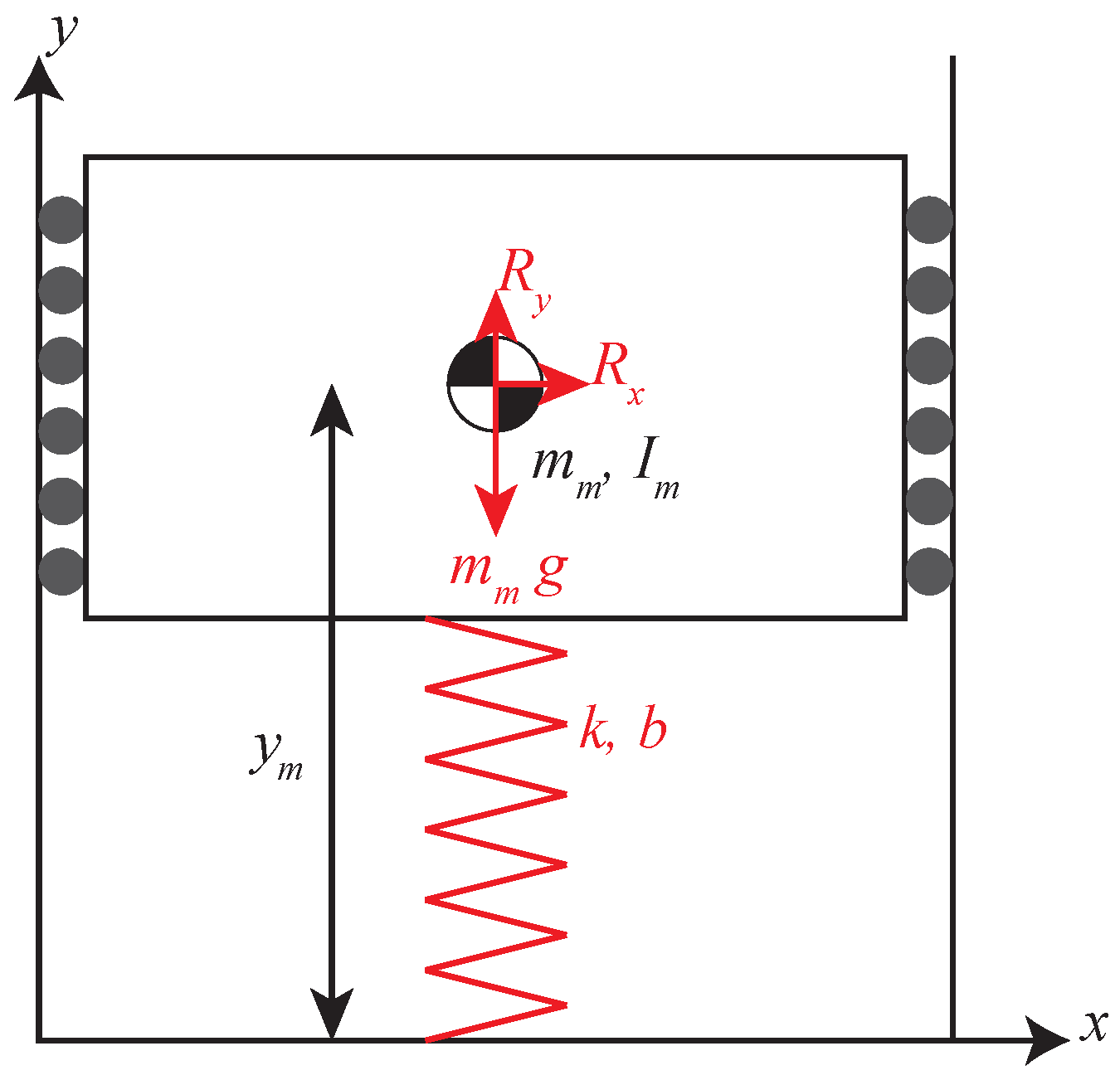
The spinner is attached at the center of mass of the robot, and the motion of the assembly is restricted in the vertical direction. The reaction forces $R_x$ and $R_y$ act on the center of mass (see Figure 2). The actuating pendulum has not been depicted in the figure in order to simplify the presentation. Instead, the inertial actuator is represented by the two reaction forces $R_x$ and $R_y$. The equation of motion for the Basketball Robot is

$$m_m{\ddot{y}}_m+(b{\dot{y}}_m+k{y}_m)S_c+m_{m}g=R_y$$

(5)

where $m_m$, $y_m$, b, k, and $S_c\in \{0,1\}$ are the main body mass, main body y-position, spring damping constant, spring elastic constant, and spring contact switch, respectively. The spring is assumed to become a rigid body while the robot is in flight. Inertial deflection of the spring while in flight is negligible.

For the rest of this subsection, let us assume the basketball robot never leaves the ground and is in ground contact ($S_c=1$).

In analysis of the Basketball Robot, changing the states given by the Newton–Euler method to the states $\ddot{\theta }$ and ${\ddot{y}}_g$ can facilitate development of analysis. By definition of the center of mass y-position as

$$\begin{array}{c}\hfill y_g=y_m-y_{m_0}-\frac{l_P{m}_{P}cos\left(\theta \right)}{m_m+m_P}\end{array}$$

(6)

$$\begin{array}{c}\hfill y_{m_0}=L_s-\frac{g(m_m+m_P)}{k}\end{array}$$

(7)

where $L_s$ is the uncompressed spring length. We define a new state $\xi$ as

$$\xi =y_m-y_{m_0}$$

(8)

Let us assume the Basketball Robot has reached a constant angular velocity. This would mean that any acceleration effects are negligible. The dynamics of the Basketball Robots height can be rewritten as

$$(m_m+m_p)\ddot{\xi }+b\dot{\xi }+k\xi =l_P{m}_{P}cos\left(\theta \right){\dot{\theta }}^2$$

(9)

With the fact that the ideal angular velocity of the spinner, ${\omega }_d$, is constant, at the ideal steady state, Equation (9) becomes

$$(m_m+m_p)\ddot{\xi }+b\dot{\xi }+k\xi =l_P{m}_{P}cos\left({\omega }_{d}t\right){\omega }_d^2$$

(10)

Equation (10) mathematically shows what has been intuitively understood. The rotational velocity of the spinners creates a sinusoidal input in the spring–mass–damper system. In a linear system, according to Bounded Input Bounded Output (BIBO), a sinusoidal input creates a sinusoid output. The closer the frequency of the input to the resonant frequency of the output, the greater the response is obtained. Equation (10) is an ordinary linear differential equation. Let us assume the following initial conditions:

$${\xi }_0=0;{\dot{\xi }}_0=0;{\theta }_0=0$$

(11)

The steady-state solution ${\xi }_s$ is

$$\begin{array}{cc}\hfill {\xi }_s& ={\xi }_{m}sin({\omega }_{d}t+\varphi )\hfill \end{array}$$

(12)

$$\begin{array}{cc}\hfill {\xi }_m& =\sqrt{\frac{l_P^2{m}_P^2{\omega }_d^4}{b^2{\omega }_d^2+{(k-(m_m+m_P){\omega }_d^2)}^2}}\hfill \end{array}$$

(13)

$$\begin{array}{cc}\hfill \varphi & ={tan}^{-1}\left(\frac{k-(m_m+m_P){\omega }_d^2}{b{\omega }_d}\right)\hfill \end{array}$$

(14)

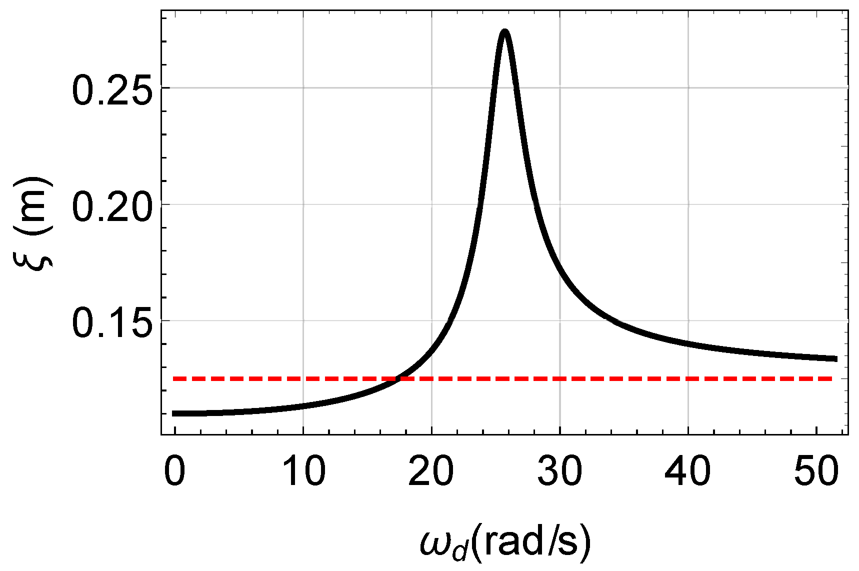
Using the first and second derivative tests, the resonant frequency ${\omega }_r$ is

$${\omega }_r=\frac{k}{\sqrt{-(b^2/2)+k(m_m+m_P)}}$$

(15)

To find the maximum response ${\xi }_r$ for the system, we substitute the ${\omega }_r$ into ${\xi }_m$:

$${\xi }_r=\frac{2k{l}_P{m}_P}{b}\sqrt{\frac{1}{4k(m_m+m_P)-b^2}}$$

(16)

Using the parameters from the Basketball Robot [22], the theoretical maximum response is at 25.7 rad/s, with a maximum response amplitude of 0.274 meters (Figure 3).

At large responses, this analysis fails because the inertial forces are large. However, at low frequencies, this analysis can be used to identify what frequency will cause the robot to start jumping or whether the robot will jump at all. If we set the steady state response of Equation (15) to the spring length (horizontal dashed line in Figure 3), then we can find the critical frequency, which will cause the robot to start jumping. For the Basketball Robot, ${\omega }_d>17.4$ rad/s.

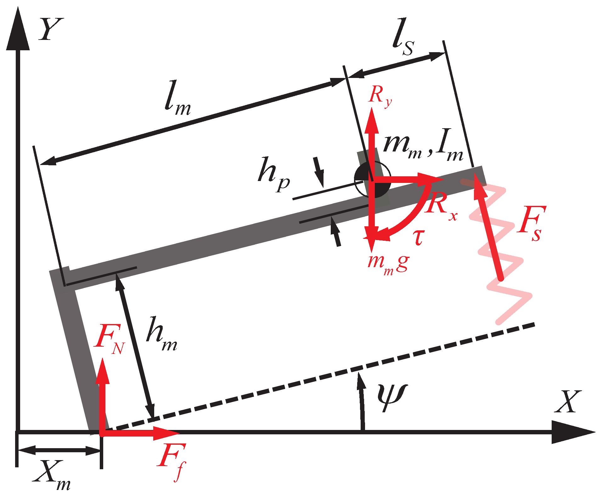
2.1.3. Tapping Robot

We are assuming that there are two conditions. The first condition occurs when the back pivot point of the robot (see Figure 4) is fixed and ${\dot{X}}_m=0$. The second condition occurs when the robot’s back pivot point is sliding and has overcome static friction at the back pivot point. The case where the back pivot point loses contact with the ground is ignored as most of the dynamics occur near the springs. Initial experimentation and simulation did not show the back pivot point loses contact with the ground. Therefore, we chose to adopt this simplification.

The constant angular velocity assumption can be applied to Tapping Robot when ${\dot{X}}_m=0$. The following transformations, symbolic calculations, and linearization are applied to the dynamics of Tapping Robot in this condition:

• Set $\ddot{\theta }$ and $\tau$ to be zero because in the constant angular velocity assumption, the angular acceleration is zero, and, accordingly, the input torque is zero.
• Replace $\dot{\theta }$ as ${\omega }_d$, which is the desired angular velocity achieved at the ideal steady state.
• Replace $\theta$ as ${\omega }_{d}t$ because the angular velocity is constant.
• Linearize the dynamics of Tapping Robot in the no sliding mode about $\psi =0$ because this is approximately the static equilibrium state for Tapping Robot.

The steps above produce a linearized version of the Tapping Robot. The transient response is ignored because the focus of this analysis is in the steady state. Applying the steps in constant angular velocity solution, the transition and resonant frequencies are approximately 35.3 rad/s and 49.0 rad/s, respectively.

3. Controller Design

The control scheme that will be used in this paper is based on a self-tuning adaptive feedback linearization approach with parameter identification.

3.1. Off-Line Spinner Parameter Identification

The success of Tapping Robot controller in this paper depends on the accuracy of the estimated parameters of the partial feedback linearization. The first step in estimating the required parameters is to find the parameters isolated to the spinner. To find these parameters, a self-tuning adaptive controller is used. One advantage of the control scheme provided in this paper is that angular acceleration is not used. The desired trajectory of the spinners is a constant velocity. Therefore, only terms in the spinners’ dynamics that affect the steady state angular velocity are required to be known. We assume the spinner’s pivot is fixed and the dynamics of the spinner given by

$$(I_P+l_p^2{m}_p)\ddot{\theta }+l_p{m}_{p}gsin\left(\theta \right)=\tau$$

(17)

In experimentation, there is an offset of origin for $\theta$, such that $\theta =\widehat{\theta }+\delta \theta$. The dynamics can be expanded as follows:

$$sin(\widehat{\theta }+\delta \theta )=cos(\widehat{\theta })sin\left(\delta \theta \right)+cos\left(\delta \theta \right)sin(\widehat{\theta })$$

(18)

Substituting the offset into the dynamics and solving for u signal from the MCU (microcontroller unit), in Equation (4), as the input:

$$\begin{array}{c}\hfill {\mathbf{\varphi }}^T\mathit{f}=u\end{array}$$

(19)

$$\begin{array}{c}\hfill \mathbf{\varphi }=\left[\begin{array}{c}\frac{I_p^{*}}{C_1{C}_2}\\ \frac{R_g}{C_2}\\ \frac{g{l}_p{m}_{p}cos\left(\delta \theta \right)}{C_1{C}_2}\\ \frac{g{l}_p{m}_{p}sin\left(\delta \theta \right)}{C_1{C}_2}\end{array}\right];\mathit{f}=\left[\begin{array}{c}\ddot{\theta }\\ \dot{\theta }\\ sin(\theta -\delta \theta )\\ cos(\theta -\delta \theta )\end{array}\right]\end{array}$$

(20)

where

$$C_1=\frac{\eta R_g}{T_s};C_2=\frac{V_b}{100}{K}_v;I_p^{*}=I_p+l_p^2{m}_p$$

(21)

We should note that $\delta \theta$ is an experimental sensor angle offset. Let us consider the following lemma [24]:

Lemma 1. 

Consider two signals e and $\mathbf{\varphi }$ related by the following dynamic equation:

$$e=H\left(s\right)\left(k{\mathbf{\varphi }}^{\mathit{T}}\mathit{v}\right)$$

(22)

where e is a scalar output signal, $H\left(s\right)$ is a strictly positive real transfer function, k is an unknown constant with known sign, $\mathbf{\varphi }$ is an $m\times 1$ vector function of time, and $\mathit{v}$ is a measurable $m\times 1$ vector. If the vector $\mathbf{\varphi }$ varies according to

$$\dot{\mathbf{\varphi }}=-sgn\left(k\right)\gamma e\mathit{v}$$

(23)

with γ being a positive constant, then e and $\mathbf{\varphi }$ are globally bounded. Furthermore, if $\mathit{v}$ is bounded, then $e\to 0$ as $t\to \infty$.

Let us define the input u as

$$u={\widehat{\mathbf{\varphi }}}^T\mathit{f}-\lambda e$$

(24)

where $\widehat{\mathbf{\varphi }}$ as the estimation vector of $\mathbf{\varphi }$. $\lambda$ is the proportional gain in the adaptive controller. This gain is tuned such that lead the estimate states converge in minimum time. The error e can be given as follows:

$$\widehat{\mathbf{\varphi }}=\left[\begin{array}{c}0\\ {\widehat{a}}_2\\ {\widehat{a}}_3\\ {\widehat{a}}_4\end{array}\right];e=\dot{\widehat{\theta }}-{\omega }_d$$

(25)

Note that ${\widehat{a}}_i;i:\{2,3,4\}$ is the estimation of each element of the vector $\mathbf{\varphi }$ in Equation (20). ${\widehat{a}}_1$ is neglected because the desired response is a constant velocity. When $e\to 0$, the $\ddot{\theta }\to 0$. Therefore, ${\widehat{a}}_1$ is not important for the desired response and can be left out. By substituting the input in Equation (24) into (19), we have

$$\lambda e={\tilde{\mathbf{\varphi }}}^T\mathit{f}$$

(26)

where

$$\tilde{\mathbf{\varphi }}=\widehat{\mathbf{\varphi }}-\mathbf{\varphi }$$

(27)

Let us define an adaptation law:

$$\dot{\tilde{\mathbf{\varphi }}}=-\mathbf{\gamma }e\mathit{f}$$

(28)

where

$$\mathbf{\gamma }=\left[\begin{array}{cccc}0& 0& 0& 0\\ 0& {\gamma }_1& 0& 0\\ 0& 0& {\gamma }_2& 0\\ 0& 0& 0& {\gamma }_2\end{array}\right]$$

(29)

Here, the components of $\mathbf{\gamma }$ are the feedback gains of the adaptation law and ${\gamma }_2$ is repeated because the adaptation of ${\widehat{a}}_3$ is very similar to ${\widehat{a}}_4$, as the sinusoidal function is the cosine function with a shift of $\frac{\pi }{2}$. Therefore, the difference in learning settling time of ${\widehat{a}}_3$ and ${\widehat{a}}_4$ should be insignificant.

Lemma 1 can be applied to this controller. Let $H\left(s\right)=\frac{1}{\lambda }$, k be selected as unity, and $\mathit{f}$ be $\mathit{v}$. The proportional gain, $\lambda$ can be moved to the right hand side of Equation (26):

$$e=\frac{1}{\lambda }{\tilde{\mathbf{\varphi }}}^T\mathit{f}$$

(30)

Which becomes

$$e=H\left(s\right)(k{\tilde{\mathbf{\varphi }}}^T\mathit{v})$$

(31)

Next, let $\tilde{\mathbf{\varphi }}$ in Equation (26) be $\mathbf{\varphi }$ in Equation (22) in Lemma 1. Therefore, Equation (26) is mathematically equivalent to Equation (22). Furthermore, the adaptive gains in $\mathbf{\gamma }$ are positive. Therefore, Equation (28) is mathematically equivalent to Equation (23) in Lemma 1 and $\dot{\theta }\to {\omega }_d$ as $t\to \infty$. Even more importantly, because $\dot{\theta }$, $sin\left(\theta \right)$, and $cos\left(\theta \right)$ are independent of each other, having a desired trajectory that is a constant speed results in a convergence of $\widehat{\mathbf{\varphi }}$ to the actual parameters of $\mathbf{\varphi }$, excluding the first element. By using this controller, off-line of the actual operation, the parameters for the partial feedback linearization of the control law in Equation (24) can be estimated.

3.2. Partial-State Feedback Linearization Controller Design during Contact Mode

To reach a practical steady state, a state feedback linearization must be used to cancel out the significant nonlinearities.

Let us consider that the robot is in contact with the springs. In Section 3.1, we found the parameters dependent only on the spinner. With $\widehat{\mathbf{\varphi }}$, we can cancel out the spinner-dependent nonlinearities. A block diagram of this feedback linearization controller is shown in Figure 5 ([25]), where

$$\begin{array}{cc}\hfill u_v& ={\lambda }_k({\omega }_d-\dot{\theta })\hfill \end{array}$$

(32)

$$\begin{array}{cc}\hfill u& =\widehat{\mathbf{\varphi }}\mathit{f}-u_v\hfill \end{array}$$

(33)

where ${\lambda }_k$ is the controller gain, $u_v$ is virtual input after linearization, and $\mathit{f}$ is the system model equation.

Assuming that we have perfect knowledge of the parameters of the system and the accelerations of the body (${\ddot{X}}_b$,${\ddot{Y}}_b$) are insignificant, the spinner’s dynamics become linear. At steady state, the response in Equation (15) can be used. The case where the back pivot point looses contact with the ground is ignored as the majority of the dynamics occur near the springs. The initial experimentation did not show the back pivot point loose contact with the ground.

3.3. Spring Compensator Design

When ground contact is lost and the robot is in flight, the force created by the springs disappears from the dynamics. This is a discontinuity that causes a lost of input/output resonance. We artificially reintroduce, through the controller, the spring forces to restore resonance (as discussed in Section 2.1.2). To do so, first, we solve Equations (1), (2), and (5) for $\ddot{\theta }$ in both modes. The corresponding dynamical equation of $\ddot{\theta }$ for contact and flying modes are given as follows:

$$\begin{array}{cc}\hfill {\ddot{\theta }}_c& =I_r(\tau +\frac{l_p^2{m}_p^{2}sin\left(2\theta \right){\dot{\theta }}^2}{2(m_m+m_p)}-\frac{l_p{m}_{p}k(L_s-y_m)sin\left(\theta \right)}{{(m_m+m_p)}^2})\hfill \end{array}$$

(34)

$$\begin{array}{cc}\hfill {\ddot{\theta }}_f& =I_r(\tau +S_P+\frac{l_p^2{m}_p^{2}sin\left(2\theta \right){\dot{\theta }}^2}{2(m_m+m_p)})\hfill \\ \hfill I_r& =\frac{2(m_m+m_p)}{2m_m(I_p+l_p^2{m}_p)+m_p(2I_p+l_p^2{m}_p)+l_p^2{m}_p^{2}cos\left(2\theta \right)}\hfill \end{array}$$

(35)

where $S_P$ is a “spring compensator” that will restore resonance. Now, we set ${\ddot{\theta }}_c={\ddot{\theta }}_f$ and solve for $S_P$.

$$S_P=\frac{k{l}_p{m}_p(L_s-y_m)sin\left(\theta \right)}{m_m+m_p}$$

(36)

Due to the fact that this system is highly nonlinear, the performance of the spring compensator can only be fully analyzed by numerical simulations. This leaves the final feedback linearization controller for the Basketball Robot (Equation (33)):

$$u=\widehat{\mathbf{\varphi }}\mathit{f}+(1-S_c)\frac{k{l}_p{m}_p(L_s-y_m)sin\left(\theta \right)}{m_m+m_p}-u_v$$

(37)

The parameters are found off-line. The parameters for $\widehat{\mathbf{\varphi }}$ are found using the adaptive feedback system identification from Section 3.1. The parameters for the spring compensator are found by tuning.

3.4. Controller Applied to Tapping Robot

A shortcut to the feedback linearization designed in the previous section is to simply replace the spring force term in the spinner dynamics with a virtual spring force, when the springs have lost contact with the ground. In order to do so, the following design algorithm must be used:

1.

Assign two different systems. The first system, ${\ddot{\theta }}_c$, is the dynamics of the spinner, while in contact with the ground. The second system, ${\ddot{\theta }}_f$, is the dynamics of the spinner, while the springs are not in contact with the ground.

2.

Define the input as

$$u=\widehat{\mathbf{\varphi }}\mathit{f}+(1-S_c)S_P-u_v$$

(38)

3.

Substitute the input into the two systems, with $S_c$ defined accordingly.

4.

Solve for $S_P$.

5.

Set the damping constant to zero in the solution because we are not measuring $\dot{\psi }$.

For Tapping Robot, with the parameters substituted (Appendix A 

Table A2. Tapping Robot parameters.

Parameter	Value	Unit	Parameter	Value	Unit
$m_p$	0.167	Kg	b	5	N.s/m
$m_m$	1.62	Kg	$L_s$	0.087	m
$l_p$	0.042	m	${\mu }_s$	0.3	-
$I_P$	0.0004	Kg.m${}^2$	${\mu }_k$	0.25	-
$I_m$	0.015	Kg.m${}^2$	$\delta \theta$	0.4485	rad
$l_s$	0.0635	m	$\eta$	0.8	-
$l_m$	0.305	m	$K_v$	41.47	rad/(s.V)
$h_m$	0.107	m	$R_g$	5.8	-
$h_P$	0.003	m	$T_s$	4921.83	rad/(m.N.s)
k	3600	N/m	$V_b$	11.6	V

):

$$\begin{array}{cc}\hfill S_P& =\hfill \\ & -\frac{6250(tan(\psi )+0.0560)(-2.76sin(\theta )+cos(\theta )-0.978)}{-2.76sin\left(\theta \right)+cos\left(\theta \right)-132}\hfill \end{array}$$

(39)

4. Simulation Results

Mathematica’s NDSolve function was used for numerically solving the differential equation. All options were used at their default setting. The sensor feedback and control law was continuous.

4.1. Off-Line Spinner Parameter Identification

In the simulation of the off-line parameter identification, the parameters for the spinner in Tapping Robot were used (See Appendix A Table A2). Other parameters include ${\gamma }_1=0.02$, ${\gamma }_2=0.2$, $\lambda =10$, and ${\omega }_d=5$ rad/s. Figure 6a–d shows the convergence of the spinner’s error to zero and the estimated parameters. ${\widehat{a}}_2$ and ${\widehat{a}}_3$ are the gravitational terms, composed of the $sin\left(\theta \right)$ and $cos\left(\theta \right)$, respectively. ${\widehat{a}}_4$ is the back electromotive force of the motor.

4.2. Basketball Robot Simulation Results

The simulation section of the Basketball Robot is structured according to increasing the sophistication of the controller design until the jumping of the Basketball Robot is stabilized.

4.2.1. Effects of Partial Linearization

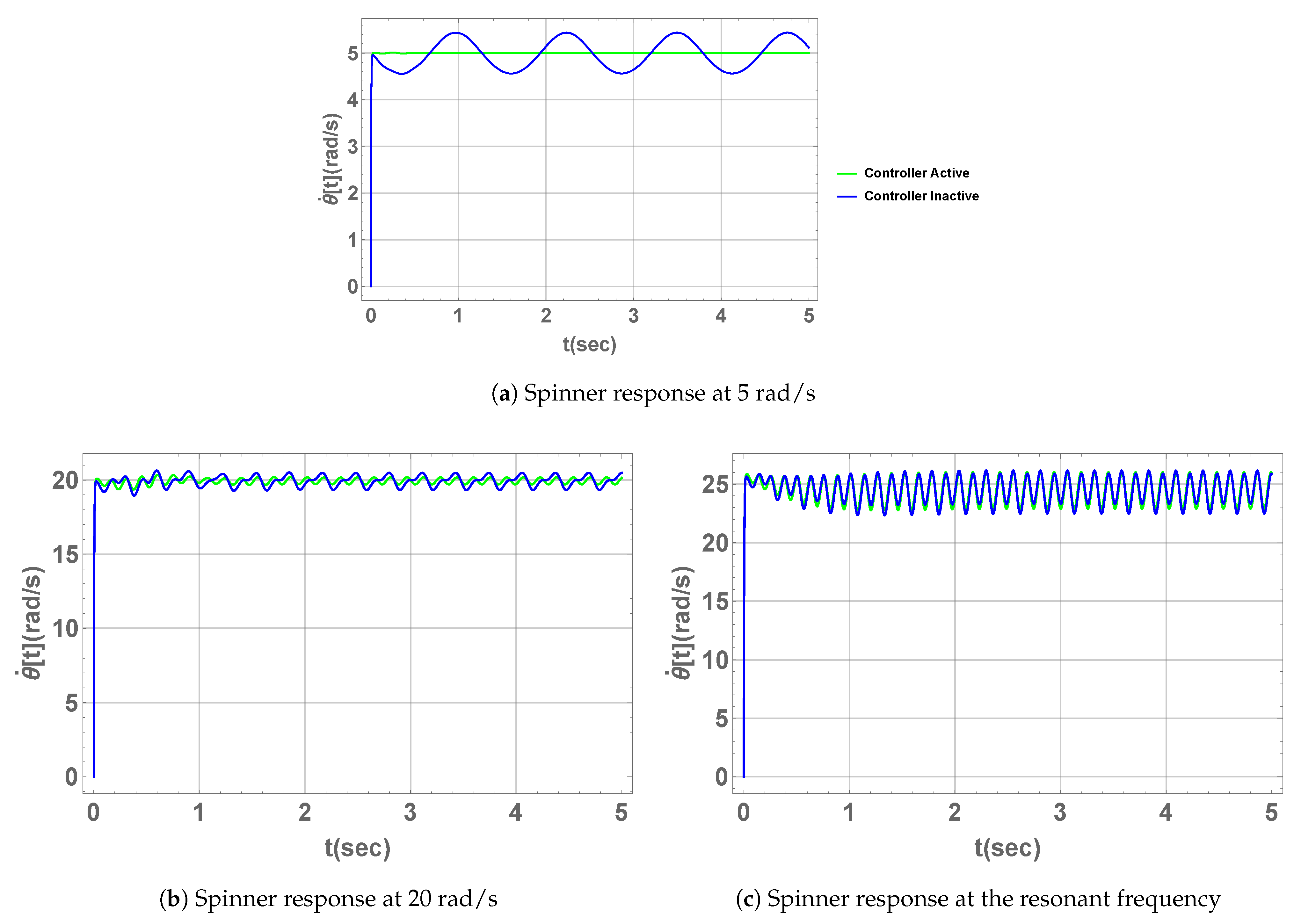
Let us first analyze the dynamics of the Basketball Robot while it is in contact with the ground. We show the results of the Basketball Robot when the partial linearization term $\widehat{\mathbf{\varphi }}\mathit{f}$ term is ignored and activated in the controller. For the simulations in Figure 7, the blue curve is the response of the Basketball Robot when the partial feedback linearization is ignored, and the green curve is when it is activated. At higher speeds, other nonlinear terms emerge to effect its performance.

4.2.2. Response at Resonant Frequency

When we change ${\omega }_d$ to 25.7 rad/s, which is the resonant frequency $\left({\omega }_r\right)$ calculated from Equation (16), we get the response for the spinners velocity and $y_m$ in Figure 7c and Figure 8c.

Furthermore, Figure 7c depicts how much the actual spinner velocity deviates from the model. In this case, the spinner has a maximum error of 2.79 rad/s or 12.2% of the modeled response. Figure 8c shows how much the actual $y_m$ deviates from the model. The red line is the maximum response amplitude calculated from Equation (16). One can see that the Basketball Robot greatly outperforms the model. The robot has a maximum error of 0.0638 m and 28%. This shows that at a certain point, the rotational acceleration of the spinners, as an input to the $y_m$ dynamics, adds to the response. Therefore, to calculate the expected response, numerical simulations must be performed.

4.2.3. Effects of Partial Linearization, Jumping, with No Spring Compensation

Now, we let the Basketball Robot loose contact with the ground. In Figure 9a, ${\lambda }_k=10$, and ${\omega }_d$ is the resonant frequency calculated from Equation (16). There appears to be an unpredictable oscillation of jumps.

4.2.4. Full Controller Response

Let us simulate the Basketball Robot with the same parameters as the simulation in Section 4.2.3, but now with the spring compensator.

Figure 9b shows the stable oscillations in steady state condition. The maximum spring deflection, at steady state, has an amplitude of 0.047 meters. As one can see in Figure 8c, maximum spring deflection occurs using the resonant frequency and it is 0.133 meters. This means that the spring should be able to store more energy at the resonant frequency. We can try adjusting ${\lambda }_k$. Let us set ${\lambda }_k$ to 0.1 and Figure 9c shows the response. Figure 9d shows the stable periodic oscillations achieved by this controller. Notice that the variables in Figure 9d are in terms of the center of mass.

We can claim that by changing ${\lambda }_k$, we can change the performance.

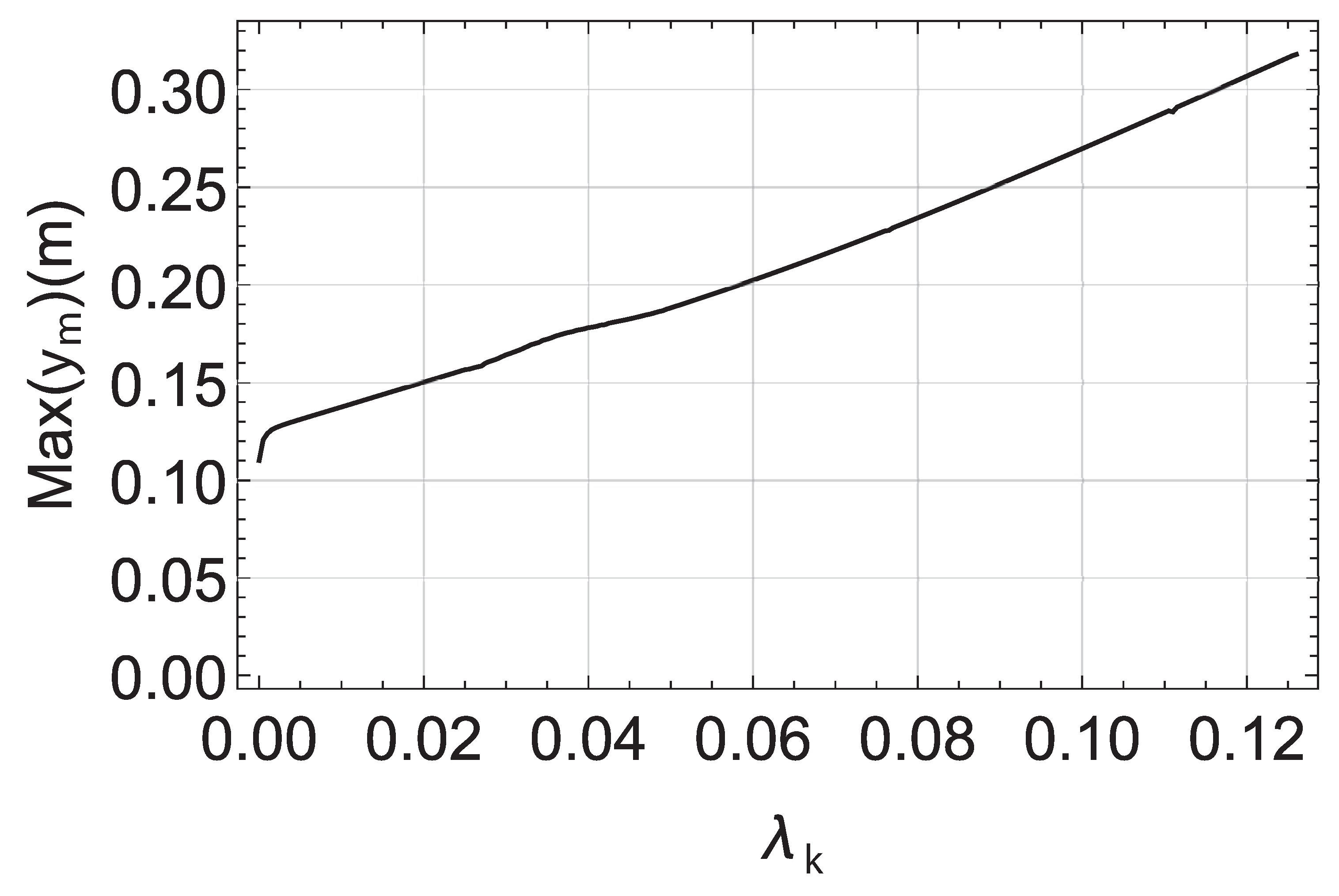
Figure 10 was obtained by simulating the system at its resonance frequency and varying ${\lambda }_k$ between 0 and 0.13, and calculating the maximum response in the last two seconds of the simulation. The last two seconds were arbitrarily chosen to be in steady state condition. There is a monotonically increasing relationship from the point the robot begins to jump and its maximum at ${\lambda }_k=0.13$. As a side note, one can adjust both ${\lambda }_k$ and ${\omega }_d$ to theoretically achieve bigger jumps, but this is not physically feasible. Ignoring physical limitations, simulations show this controller can achieve a jump height of 0.86 meters (see Figure 11).

Figure 10 can be used to prescribed the jump height of the basketball robot by choosing the appropriate values of ${\lambda }_k$. This is the desired response of the Feedback Linearization Controller applied to the Basketball Robot.

4.3. Stability Analysis

In this section, we analyze the stability of the system in neighborhoods of equilibria. In this regard, we use Poincaré Map and Floquet Theory. Because the closed form analytic solution of differential equations of motion is not available, numerical integration is used [13]. Let $q\left(t\right)$ be the the periodic solution of the equations of motion for all states. The simplified hyperplane of the Poincaré section can be defined as

$$\mathfrak{S}=(y_m,\theta ,\dot{\theta })\in R^3;{\dot{y}}_m=0$$

(40)

If $q\left[k\right]\in \mathfrak{S}$ denotes the $k^{th}$ intersection of $\mathfrak{S}$ by the flow of $q\left(t\right)$ the discrete-time Poincaré Map $\mathfrak{P}:\mathfrak{S}\to \mathfrak{S}$ can be expressed as

$$q[k+1]=\mathfrak{P}\left(q\right[k\left]\right)$$

(41)

Subsequently, if $q^{*}$ stands for the fixed point of the Poincaré Map, then the local exponential stability of $q^{*}$ on $\mathfrak{S}$ is equivalent to local exponential stability of the underlying limit cycle. We used Floquet Theory for stability analysis of limit cycles [15,16]. In this regard, the local linearization of the Poincaré Map about its fixed point yields

$$\begin{array}{ccc}& & \mathfrak{P}\left(q\right)\simeq \mathit{J}\left(q^{*}\right)(q-q^{*})\hfill \\ & & \mathit{J}=\frac{\partial \mathfrak{P}\left(q\right)}{\partial q}\hfill \end{array}$$

(42)

where J is $3\times 3$ linearized Jacobian matrix of $\mathfrak{P}$

$$J=\left[J_{i,j}\right];J_{i,j}=\frac{\partial \mathfrak{P}}{\partial q_i}$$

(43)

Then, the floquet or characteristic multipliers ${\rho }_i$’s are defined as eigenvalues of the Jacobian matrix J

$${\rho }_i=∥{\lambda }_i∥;{\lambda }_i=\mathrm{eig}\left(J\right)$$

(44)

where, ${\rho }_i$ and ${\lambda }_i$ are the $i^{th}$ characteristic multiplier and Jacobian matrix eigenvalue, respectively, and $‘‘∥∥"$ is the modulus operator. Therefore, the limit cycle stability can be identified by Floquet multiplier metrics as

$$q\left(t\right)=\left\{\begin{array}{cc}\mathrm{stable}& \forall ∥{\rho }_i∥<1\\ \mathrm{marginally}\mathrm{stable}& \forall ∥{\rho }_i∥=1\\ \mathrm{unstable}& \forall ∥{\rho }_i∥>1\end{array}\right.$$

(45)

As Kashki et al. [22] showed, the system has periodic motion, we can use the Poincaré Map and Floquet Theory. The Floquet multipliers associated with the corresponding Poincaré map for the simulations are calculated numerically as:

$$\begin{array}{cc}& {\rho }_1=∥{\lambda }_1∥=0.3866<1\hfill \\ & {\rho }_2=∥{\lambda }_2∥=0.0425<1\hfill \\ & {\rho }_3=∥{\lambda }_3∥=0.0087<1\hfill \end{array}$$

(46)

All norms of characteristic multiplier of the system are less than one, which means that the limit cycle is asymptotically stable.

4.4. Tapping Robot Simulation Results

The following are the results of the dynamics and controller provided in this paper for Tapping Robot.

Figure 12 depicts the response of Tapping Robot, when the robot is run at the transition frequency ${\omega }_d=35.3$, and ${\lambda }_k=0.5625$, and also the response at the Pseudostable condition which is ${\omega }_d=39$ and ${\lambda }_k=0.003$. In simulation, the spring compensator approach did not lead to stable periodic orbits. Therefore, for the results shown, the partial feedback linearization of Equation (38) was used with $S_c=1$. For the feedback linearization scheme, however, a value of ${\omega }_d=39$ rad/s has led to a stable limit cycle. The response reaches steady state at 6.5 s. As desired, a stable periodic progression of the Tapping Robot has been achieved.

5. Experimental Setup

5.1. Mechanical Components

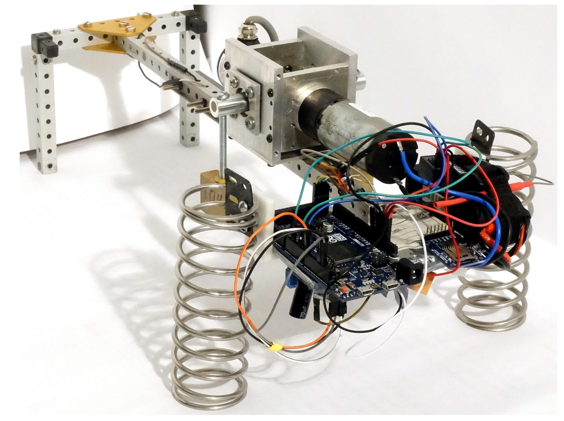
In Figure 13 and Figure 14 are photographs of the Tapping Robot. The main components of Tapping Robot are the spinners, the frame, and the springs. The spinners were custom-machined to be interchangeable with different masses. In the experiment, two 104 gram brass weights were locked onto two 3′′ 10–32 machine screws. The two spinners were coupled together inside the gearbox, such that they spin together, essentially creating a single spinner. Inside the gearbox, there are miter gears linked together. The back miter gear connects to an incremental encoder with an index. The middle miter gear connects to the spinner. The front miter gear connects to the motor. The frame came from an aluminum erector set. The springs are custom made oppositely wound springs with a total spring constant of 3600 N/m (Hanson Springs, Dallas, TX, USA). The two springs have opposite windings to cancel out any moments created by their compression. The free length and the outer diameter are 127 mm and 49.2 mm, respectively.

The rotational sensor is a model GHS38-6G1024BML5 rotary encoder (CALT, Baoshan District, Shanghai, China). The encoder has an 6mm shaft and 1024 Pulse/Revolution resolution. This creates a 0.0879${}^{\circ }$ resolution using a quadrature decoder function on the Due microcontroller (Arduino, Ivrea, Italy). The encoder has an index output triggered every revolution. This prevents a drift in the position reading. The encoder is linked to the system through the miter gear.

The miter gears are 25 Teeth, 1 Module, ISO 8 /Brass Miter Gears(SDP\SI, Hicksville, NY, USA). They are greased to reduce vibrations. The middle miter gear is secured to the shaft with a setting screw coated in Loctite 242.

Due to the high torques required in the robot, the A-max 32, Graphite Brushes, 15 Watt, with terminals was selected (Maxon Motor AG, Sachseln, Switzerland). To increase the available torque, the motor was attached to a Planetary Gear-head GP 32 A Ø32 mm, 0.75–4.5 Nm, Metal Version. The motor has a nominal voltage of 12 volts; a no-load speed of 4680 rpm; stall torque of 101 mNm; and a maximum efficiency of 77%. The gearbox has a gear ratio of 5.8:1; a maximum continuous torque of 0.75 Nm; and a maximum efficiency of 80%.

5.2. Electrical Components

In Figure 15 is the electrical circuit diagram of the Tapping Robot. The entire controller is run on an Arduino Due. All digital pins have interrupts for encoders. To power the robot a Turnigy Graphene 1300mAh 3S 45C LiPo Pack w/ XT60 is used (HobbyKing, Kowloon, Hong Kong, China). The lithium polymer has an operating voltage of 9 to 12.6 volts. The power is sent from the batteries to the motor driver. The motor driver used is a G2 High-Power Motor Driver 18v17 (Pololu Corporation, Las Vegas, NV, USA). The motor driver can provide a continuous output current of 17 Amps. A RC Receiver is added to provide direct control of the robot. Navigation is controlled by the user through the RC transmitter/receiver. The RC transmitter is the FS-T6 6-channel transmitter and the RC receiver is the FS-R6B 6-channel receiver (Shenzhen Flysky Technology Co.,Ltd., Shenzhen, China).

5.3. Data Acquisition

The data gathered for the Tapping Robot experiment was captured by a RX100V point-and-shoot camera (Sony, Minato City, Tokyo, Japan) for a 2 dimensional image. The video was shot at 70 mm 35 mm-equivalent focal length. The video was shot at 960 fps and 1920 × 1080 pixel resolution. The data gathered for the fixed spinner experiment were captured a direct serial com-port to a computer.

6. Experimental Results

6.1. Off-Line Spinner System Identification

One assumption of the model for the spinner is that the spinner is fixed at its pivot point. Therefore, in performing the off-line spinner parameter identification (Section 3.1), the frame of robot was fixed to a table.

Three different experiments were run with different initial conditions. The curves corresponding to each set of initial conditions is shown in

Table 1. Spinner System Identification Initial Conditions.

Experiment No.	1	2	3
${\widehat{a}}_2\left[0\right]$	0	10	30
${\widehat{a}}_3\left[0\right]$	10	20	30
${\widehat{a}}_4\left[0\right]$	0	0	2.3

.

Results

Figure 16 shows the convergence of the spinner’s error to 0 and the estimated parameters. According to the specifications of the Maxon motor, the speed constant is 1.165%/(rad/s). However, as shown by the plot, the controller levels off at 2%/(rad/s). Other experimentation showed that there exists a friction force that is constant and not related to the angular velocity. This results in a steady-state error for the estimated speed constant. One can see the video of this experiment as a Supplementary Material to this paper.

6.2. Tapping Robot

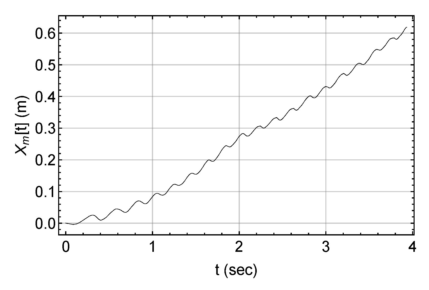
The Tapping Robot was run at ${\omega }_d$ = 36 rad/s and ${\lambda }_k$ = 0.5625. The experiment in Figure 17 shows a steady forward progression of Tapping Robot. This is the desired result of this paper and shows the controller has been successful. In comparison to the simulation in Figure 12b, the robot has a stronger periodic oscillation in its progression. This can be seen in the velocity plot in Figure 18. In the simulation, Tapping Robot’s velocity is never negative, where as in the experiment, the robot slides forwards and backwards. One can see the video of this experiment as a supplementary material to this paper. Like the simulation, the partial feedback linearization of Equation (38) was used with $S_c=1$. The spring compensator was not active because the sampling rate of the rangefinder was insufficient for successful controller action.

7. Discussion

While inertially actuated jumping robots promise speed and maneuverability, the work in this paper shows the complexity for controlling them. In research of IAJR up to this point, basketball robots and tapping-like robots have been achieved and controlled. The previous controller applied to the basketball robot achieved a maximum jump height of 0.18 m. As shown in simulations, the controller in this paper achieved a jump height of 0.25 m. This is a 39% increase in response. The previous controller applied to a similar tapping-like robot achieved a forward progression speed of 0.045 m/s. The tapping robot presented in this paper, with the new controller applied, achieved a forward progression speed of 0.157 m/s. This is a 249% increase in performance. This paper stays consistent to previous concepts presented by our lab, but builds on it with simpler controllers and higher performance.

However, the improvements of the family of controllers presented in this paper are not only quantitative, but also structural. In [22], the adaptive controller for the Basketball robot requires a complicated control algorithm. This algorithm involves a predictive timing of when the robot will return to the ground. This method is subject to errors. The feedback linearization controller has no predictive measurements and is simpler. The input variables only needed for the feedback linearization are $\theta ,\dot{\theta },$ and $y_m$. All of which require no predictions. The structural advantage of the feedback linearization controller to the controllers used on the Pony robot is also simplicity. The two previous controllers were a PID controller and a sliding mode controller. The issue with the PID controller is it does not account for nonlinearities. Obviously, the feedback linearization controller does. Finally, the sliding mode controller requires a sliding mode term in the dynamics to account for parameter uncertainty. Because the parameters are identified offline, the feedback linearization controller does not need a sliding mode term and is simpler and faster.

There is more future work to be done. The model of the Tapping Robot requires improvement as well. Experiments showed that the back end of the robot does not stay in contact with the ground for all times. However, this is not the case for simulation. This may be the cause of the disagreement between the experimental and simulation results. Due to a slow range finder, the spring compensator was not able to be implemented in the experiment. A faster rangefinder needs to be developed and selected. A robust term needs to be added to this controller, as feedback linearization controllers are sensitive to parameter errors.

Another issue is the synchronization of the spinners in IAJR to locomotion. The periodic motion of the locomotion is dependent on the spinners inertial forces being applied in sync with the movement. This transient dynamic is outside the scope of this paper and should be investigated further.

Once Tapping Robot’s dynamics are better understood and controlled, then IAJR can be extended to more complex designs, such as the designs introduced in [17].

References

- Razzaghi, P.; Khatib, E.A.; Hurmuzlu, Y. Nonlinear dynamics and control of an inertially actuated jumper robot. Nonlinear Dyn. 2019, 97, 161–176. [Google Scholar] [CrossRef]
- Miyashita, K.; Ok, S.; Hase, K. Evolutionary generation of human-like bipedal locomotion. Mechatronics 2003, 13, 791–807. [Google Scholar] [CrossRef]
- Zhang, J.; Song, G.; Li, Y.; Qiao, G.; Song, A.; Wang, A. A bio-inspired jumping robot: Modeling, simulation, design, and experimental results. Mechatronics 2013, 23, 1123–1140. [Google Scholar] [CrossRef]
- Chen, X.; Wang, L.Q.; Ye, X.F.; Wang, G.; Wang, H.L. Prototype development and gait planning of biologically inspired multi-legged crablike robot. Mechatronics 2013, 23, 429–444. [Google Scholar] [CrossRef]
- Zhao, J.; Zhao, T.; Xi, N.; Mutka, M.W.; Xiao, L. MSU tailbot: Controlling aerial maneuver of a miniature-tailed jumping robot. IEEE/ASME Trans. Mechatron. 2015, 20, 2903–2914. [Google Scholar] [CrossRef]
- Wang, H.; Luan, Y.; Oetomo, D.; Wang, Z. Design, analysis and experimental evaluation of a gas-fuel-powered actuator for robotic hoppers. IEEE/ASME Trans. Mechatron. 2014, 20, 2264–2275. [Google Scholar] [CrossRef]
- Li, S.; Rus, D. JelloCube: A Continuously Jumping Robot With Soft Body. IEEE/ASME Trans. Mechatron. 2019, 24, 447–458. [Google Scholar] [CrossRef]
- Verrelst, B.; Vanderborght, B.; Vermeulen, J.; Ham, R.V.; Naudet, J.; Lefeber, D. Control architecture for the pneumatically actuated dynamic walking biped “Lucy”. Mechatronics 2005, 15, 703–729. [Google Scholar] [CrossRef]
- Yi, S. Reliable gait planning and control for miniaturized quadruped robot pet. Mechatronics 2010, 20, 485–495. [Google Scholar] [CrossRef]
- Wu, Q.; Chen, J. Effects of ramp angle and mass distributions on passive dynamic gait—An experimental study. Int. J. Humanoid Robot. 2010, 7, 55–72. [Google Scholar] [CrossRef]
- Raibert, M.; Blankespoor, K.; Nelson, G.; Playter, R. BigDog, the Rough-Terrain Quadruped Robot. Int. Fed. Autom. Control. 2008, 41, 10822–10825. [Google Scholar] [CrossRef] [Green Version]
- Murphy, M.P.; Saunders, A.; Moreira, C.; Rizzi, A.A.; Raibert, M. The LittleDog robot. Int. J. Robot. Res. 2011, 30, 145–149. [Google Scholar] [CrossRef]
- Hurmuzlu, Y.; GéNot, F.; Brogliato, B. Modeling, stability and control of biped robots—a general framework. Automatica 2004, 40, 1647–1664. [Google Scholar] [CrossRef] [Green Version]
- Westervelt, E.; Chevallereau, C.; Morris, B.; Grizzle, J.; Choi, J.H. Feedback Control of Dynamic Bipedal Robot Locomotion; CRC Press: Boca Raton, FL, USA, 2007. [Google Scholar] [CrossRef] [Green Version]
- Hürmüzlü, Y.; Moskowitz, G.D. Bipedal locomotion stabilized by impact and switching: I. Two-and three-dimensional, three-element models. Dyn. Stab. Syst. 1987, 2, 73–96. [Google Scholar] [CrossRef]
- Hürmüzlü, Y.; Moskowitz, G.D. Bipedal locomotion stabilized by impact and switching: II. Structural stability analysis of a four-element bipedal locomotion model. Dyn. Stab. Syst. 1987, 2, 97–112. [Google Scholar] [CrossRef]
- Zoghzoghy, J.; Zhao, J.; Hurmuzlu, Y. Modeling, design, and implementation of a baton robot with double-action inertial actuation. Mechatronics 2015, 29, 1–12. [Google Scholar] [CrossRef]
- Zoghzoghy, J.; Hurmuzlu, Y. Dynamics, stability, and experimental results for a baton robot with double-action inertial actuation. Int. J. Dyn. Control. 2018, 6, 739–757. [Google Scholar] [CrossRef]
- Kovac, M.; Fuchs, M.; Guignard, A.; Zufferey, J.C.; Floreano, D. A miniature 7g jumping robot. In Proceedings of the 2008 IEEE International Conference on Robotics and Automation, Nice, France, 22–26 September 2008; pp. 373–378. [Google Scholar] [CrossRef] [Green Version]
- Armour, R.; Paskins, K.; Bowyer, A.; Vincent, J.; Megill, W. Jumping robots: A biomimetic solution to locomotion across rough terrain. Bioinspir. Biomim. 2007, 2, S65–S82. [Google Scholar] [CrossRef] [PubMed] [Green Version]
- Weiss, P. Hop… hop… hopbots!: Designers of small, mobile robots take cues from grasshoppers and frogs. Sci. News 2001, 159, 88–91. [Google Scholar] [CrossRef]
- Kashki, M.; Zoghzoghy, J.; Hurmuzlu, Y. Adaptive Control of Inertially Actuated Bouncing Robot. IEEE/ASME Trans. Mechatron. 2017, 22, 2196–2207. [Google Scholar] [CrossRef]
- Kafader, U. The Selection of High-Precision Microdrives; Maxon Academy: Sachseln, Switzerland, 2007. [Google Scholar]
- Narendra, K.S.; Annaswamy, A.M. Stable Adaptive Systems; Prentice Hall: Upper Saddle River, NJ, USA, 1989. [Google Scholar]
- Slotine, J.J.E.; Li, W. Applied Nonlinear Control; Prentice Hall: Upper Saddle River, NJ, USA, 1991. [Google Scholar]
Figure 1.
Robot’s spinner free body diagram.
Figure 2.
Basketball Robot free body diagram.
Figure 3.
The relationship between the magnitude of the steady state response and the desired rotational velocity of the spinner.
Figure 4.
Tapping Robot’s free body diagram (FBD).
Figure 5.
Spring Contact Basketball Robot Controller.
Figure 6.
Simulation Results for Convergence of Parameters.
Figure 7.
Attached to ground, Spinner Response.
Figure 8.
Attached to ground, Basketball Robot Response.
Figure 9.
Basketball Jump Response.
Figure 10.
Basketball Robot Response Curve, .
Figure 11.
Basketball Super Jump Response, and .
Figure 12.
Tapping Robot Simulations.
Figure 13.
Top view of robot.
Figure 14.
Isometric view of experimental set up.
Figure 15.
Electrical schematic.
Figure 16.
Experimental parameter convergence.
Figure 17.
Experimental Horizontal Progression of Tapping Robot.
Figure 18.
Experimental Horizontal Velocity of Tapping Robot.