Article

Model-Based Condition-Monitoring and Jamming-Tolerant Control of an Electro-Mechanical Flight Actuator with Differential Ball Screws

by
Gianpietro Di Rito
1,*,
Benedetto Luciano
2,
Nicola Borgarelli
3 and
Marco Nardeschi
3
1
Dipartimento di Ingegneria Civile ed Industriale, Università di Pisa, 56122 Pisa, Italy
2
AESIS srl, San Giuliano Terme, 56017 Pisa, Italy
3
Umbragroup Spa, 06034 Foligno, Italy
*
Author to whom correspondence should be addressed.
Submission received: 9 July 2021 / Revised: 26 August 2021 / Accepted: 6 September 2021 / Published: 9 September 2021
(This article belongs to the Special Issue Health Monitoring and Fault Diagnosis on Actuation Systems)

Abstract

:
The work deals with the development of deterministic model-based condition-monitoring algorithms for an electromechanical flight control actuator with fault-tolerant architecture, in which two permanent magnets synchronous motors are coupled with differential ball screws in speed-summing paradigm, so that the system can operate even after a motor fault, an inverter fault or a mechanical jamming. To demonstrate the potential applicability of the system for safety-critical aerospace applications, the failure transients related to major fault modes have to be characterised and analysed. By focusing the attention to jamming faults, a detailed nonlinear model of the actuator is developed from physical first principles and experimentally validated in both time and frequency domains for normal condition and with different types of jamming. The validated model is then used to design the condition-monitoring algorithms and to characterize the system failure transient, by simulating mechanical blocks in different locations of the transmission. The operability after the fault, obtained via fault-tolerant control strategy and position regulator reconfiguration, is also verified, by highlighting and discussing possible enhancements and criticalities.

1. Introduction

1.1. Research Context

The aircraft electrification is surely one of the most important and strategic initiatives currently supporting the innovation of the aviation industry [1,2]. This manifests in two basic concepts: the more-electric aircraft and the more-electric propulsion (way to the all-electric long-term targets). In particular, the more-electric aircraft concept entails the gradual replacement of onboard systems based on mechanical, hydraulic, or pneumatic power sources with electrically-powered ones, aiming to reduce weight and costs, to optimize energy and to increase eco-compatibility and reliability of future aircrafts [3,4,5,6]. One of the key technological enablers for pursuing these challenging objectives is the electro-mechanical actuation [7,8,9]. The applicability of Electro-Mechanical Actuators (EMAs) in aerospace is well proved in terms of load and speed performances [10,11,12,13,14], but it still entails several concerns in terms of safety and reliability [15,16,17,18,19]. In civil aircrafts, EMAs are often avoided for safety-critical functions (flight controls, brakes, landing gears, nose wheel steering), essentially because the statistical database on components fault modes is poor [20]. Electrical and electronic faults are currently not critical for aerospace applications of EMAs, since they can be effectively counteracted via hardware redundancy, without significant impacts on weight and volumes [21,22,23,24,25,26]. On the other hand, mechanical faults are more problematic. The most feared fault mode is surely the mechanical jamming, which is the final consequence of the progressive degradation of loaded metallic contacts in the EMA gear train. The wear and fatigue in the materials initially imply increased friction and lower efficiency (affecting power consumption and control performances), or increased freeplay (with possible impacts on aeroservoelastic stability of flight movables), while in the long term they can lead to mechanical blocks. Potentially, the jamming of a primary flight surface is a failure with catastrophic consequences, which can make useless any architecture based on either parallel or grouped actuators. The survivability to jamming is thus one of the major challenges in the development of EMAs for safety-critical aerospace applications.
Many research efforts have been and are made to protect EMAs from jamming, by applying both prognostic and diagnostic monitoring methods, aiming at anticipating (i.e., avoiding), or detecting and isolating the fault, respectively. The prognostic solution, though potentially overwhelming [27,28,29,30], is nowadays far from being applicable to airworthy systems, so that diagnostic approaches are typically preferred [31,32].
The diagnostic monitoring requires that fault detection and isolation (FDI) algorithms are implemented and real-time executed by onboard control electronics [33,34,35,36], so that, in case of a detected jamming, redundant mechanical channels or unlock devices can be engaged [37,38]. Depending on how the mechanical redundancy is applied, after the fault compensation, the EMA can maintain its functionality, or it can be reverted in a stand-by mode, so that jamming-operative or jamming-safe EMAs are respectively obtained. In fact, for each primary flight movable, the mechanical redundancy can be applied at load-level (by splitting the movable and using a jamming-safe EMA on each part), at actuator-level (using multiple jamming-safe EMAs on a single movable), or at subsystem-level (using a single jamming-operative EMA on a single movable). The use of jamming-tolerant transmissions in EMAs clearly increases the design complexity, but it strongly simplifies the system integration with respect to architectures with multiple actuators. On the other hand, the FDI algorithms of a jamming-operative (more generally fail-operative) EMA are expected to be more sophisticated and prone to errors.

1.2. Motivations of the Research

Provided that fail-operative EMAs are the preferred solution for the primary flight controls of more-electric aircrafts, a key aspect entails the design and the verification of appropriate condition-monitoring systems. Apart from the need of limiting the number of additional sensors and algorithms, a special attention must be paid to the monitoring approach itself. Literature identifies three basic methods: knowledge-based, signal-based and model-based approaches [39,40]. In knowledge-based approaches, there is no a priori knowledge (i.e., model) of the physics-of-failure, but it is reconstructed from a large volume of historical data, by means of artificial intelligence techniques. Signal-based approaches instead utilize coarse pre-defined information about the system behaviour and the diagnostic output is directly generated by analysing the system signals. Finally, in model-based approaches, the diagnosis is obtained from the comparison of system measurements with a priori information provided by mathematical models, through the generation and analysis of residual quantities [41].
The condition-monitoring of a primary flight control EMA, which must be executed in real-time and with minimum FDI latency, surely requires a model-based approach, but different techniques can be applied. Since nonlinearities, disturbances, environment and loads can significantly affect actuators response, an in-depth knowledge of both normal and faulty behaviours is required. The crucial problem entails the knowledge of faulty dynamics and failure transients in complex systems with a huge number of fault modes.
In data-driven model-based techniques, this knowledge is achieved via experiments, by artificially injecting the major faults and measuring the system response during and after the fault [20,28,29,42,43]. This method provides more accurate predictions, but rigging costs are often prohibitive and the FDI strongly depends on tested conditions.
In deterministic model-based techniques, which this paper refers to, the knowledge of dynamics with faults is derived from a mathematical model, capable of simulating the faults occurrence by physical first-principles [33,34,35,36], which is experimentally-validated with reference to normal and/or regime faulty conditions. Oppositely to the data-driven case, this method generally provides less accurate predictions, but it is cost-effective, it allows to verify FDI functionalities in extreme conditions and (above all) permits to generalise the FDI algorithms validity to similar equipments (i.e., governed by similar equations).
The development of a high-fidelity dynamic model of an EMA and its consequent experimental validation are thus, of paramount importance for the design of a deterministic model-based condition-monitoring, especially for the failure transients characterisation (with particular reference to the ones related to jamming faults, literature information is scarce). The basic objective of this work is thus to design and validate a deterministic model-based monitoring system of a fault-tolerant EMA for primary flight controls developed by Umbragroup (Italy), aiming at demonstrating the potential applicability of the actuator for safety-critical aerospace applications. In previous works by the authors [44,45], a preliminary performance verification of the monitoring system was obtained, but the experimental validation of the model was limited to the normal condition and the accuracy in terms of motor currents response was poor. This paper substantiates the effectiveness of the condition-monitoring design, by enhancing the EMA model accuracy and extending its experimental validation in both time and frequency domains to all the system operative modes.

2. Materials and Methods

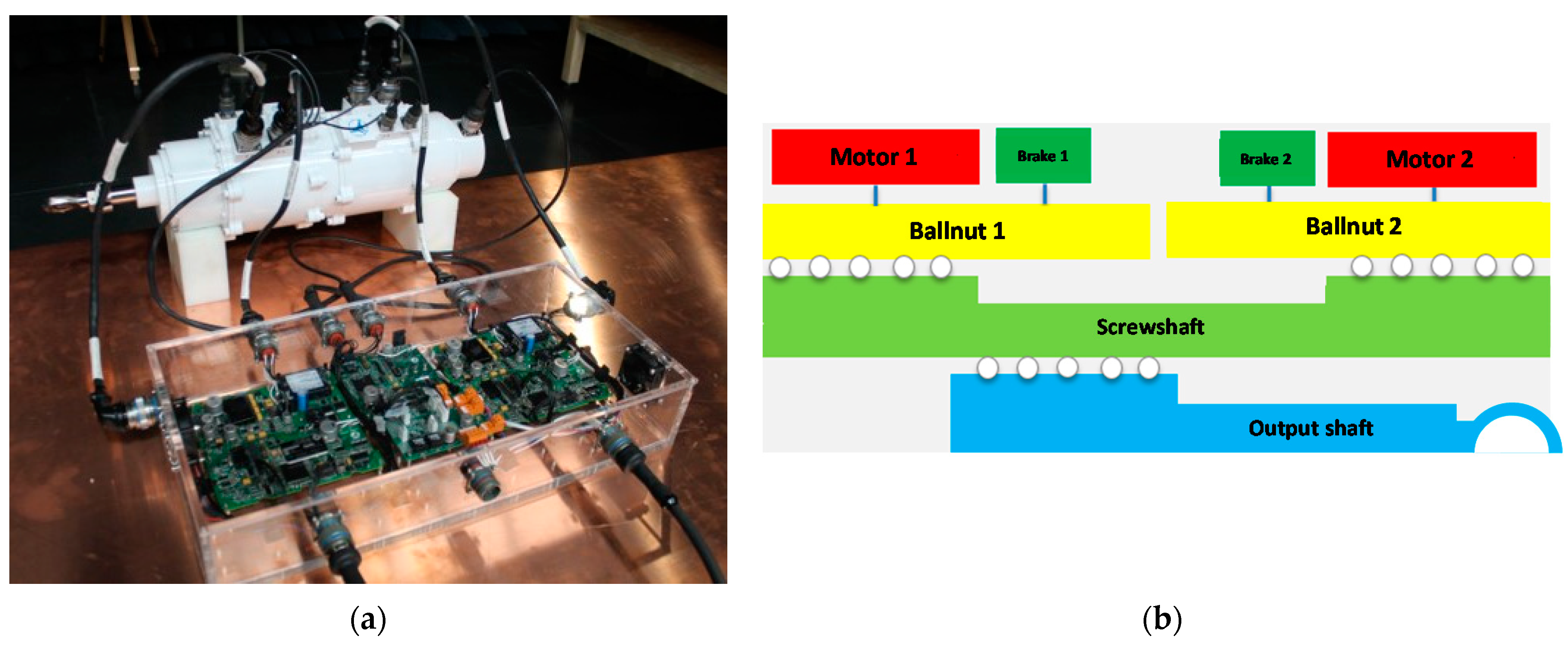
2.1. System Architecture

The reference actuator is a fault-tolerant EMA (Figure 1a), basically composed of
  • dual redundant three-phase Permanent Magnets Synchronous Machines (PMSMs) with surface-mounted magnets and sinusoidal back-electromotive forces, driven via Field-Oriented Control (FOC) technique;
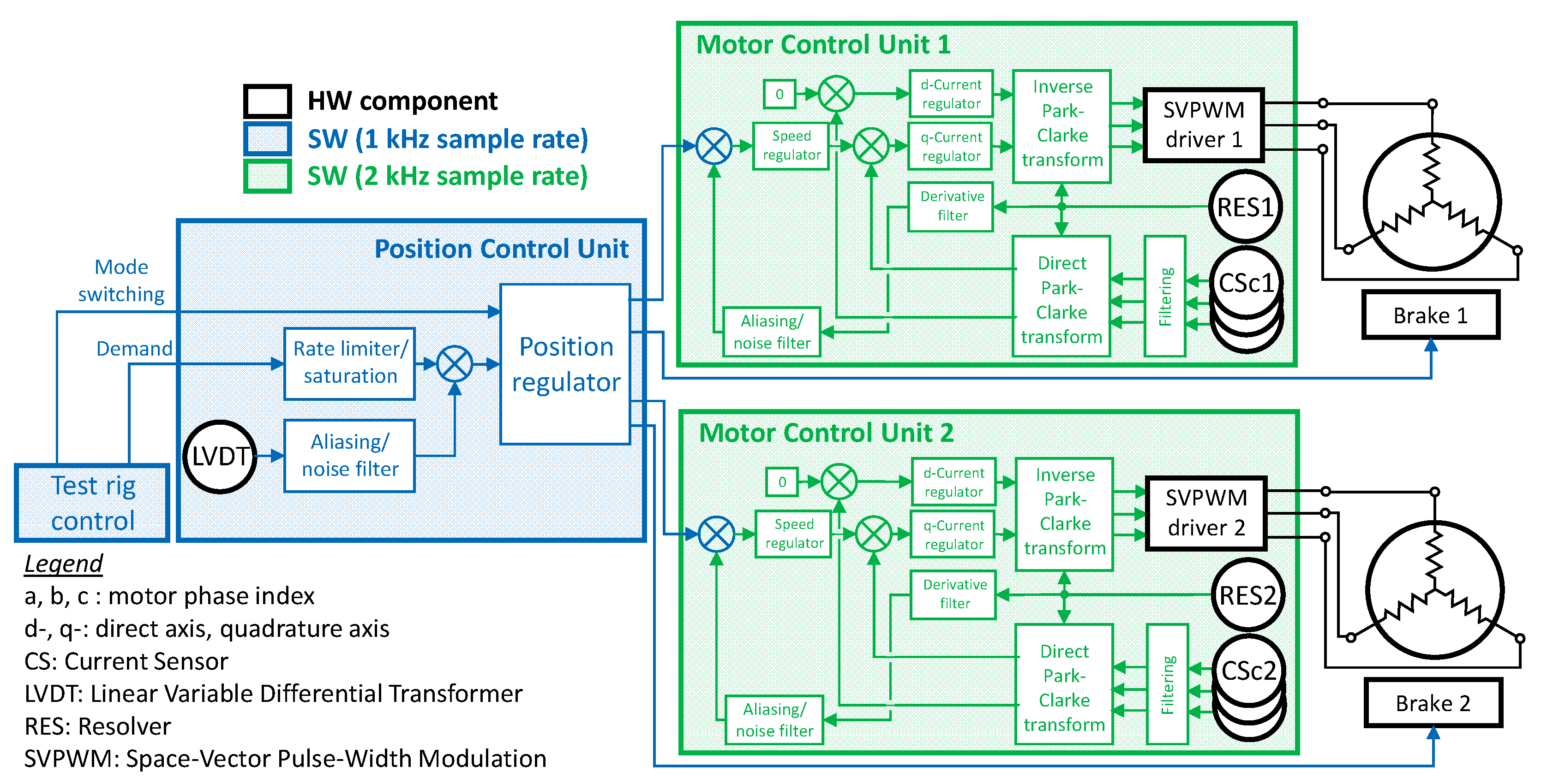
  • dual Electronic Control Units (ECUs), implementing the condition-monitoring algorithms and the closed-loop control functions, based on three nested loops on motors currents, motors speeds and output shaft position;
  • Umgragroup-patented jamming-tolerant mechanical transmission with differential ball-screws (Figure 1b).

2.2. Mechanical Transmission

The mechanical transmission of the EMA is based on differential ball-screws couplings. The two motors engage, via rotor-integrated ball-nuts, an intermediate screwshaft having three threaded portions: two external ones for the motors and an internal one for the output shaft, Figure 1b. The kinematics thus implements a speed-summing paradigm and the relationships between the motors rotational speeds ( θ ˙ 1 and θ ˙ 2 ), the output translational speed ( x ˙ o ) and the screwshaft translational and rotational speeds ( x ˙ s s and θ ˙ s s ) are given by Equations (1)–(3),
θ ˙ s s   =   p s 1 θ ˙ 1 p s 2 θ ˙ 2 p s 1 p s 2 ,
x ˙ s s   =   p s 1 p s 2 2 π ( p s 1 p s 2 ) ( θ ˙ 1 θ ˙ 2 ) ,
x ˙ o   =   b 1 θ ˙ 1   +   b 2 θ ˙ 2   =   p s 1 ( p s 2 p s 3 ) 2 π ( p s 1 p s 2 ) θ ˙ 1     p s 2 ( p s 1 p s 3 ) 2 π ( p s 1 p s 2 ) θ ˙ 2 ,
in which ps1 and ps2 are the leads of the motor screw-nut couplings and ps3 is the lead of the output shaft screw.
Theoretically, there are infinite combinations of motors motions generating the same output translation, Equation (3). However, a set of relevant combinations of motors speeds has been selected to define the EMA operative modes, Table 1.
In active/stand-by modes (ASB and SBA in Table 1), one motor rotates and the other is de-energized and held by the related brake, so that the screwshaft has a roto-translating motion, Equations (1) and (2). In active/active modes, both motors rotate and, depending on their speeds, the motion of the screwshaft can range from roto-translation to pure translation or pure rotation (AAPT and AAPR in Table 1). Among all possible active/active modes generating the screwshaft roto-translation, one implies a balanced power split among the motors in quasi-dynamic regime (i.e., at constant motors speeds). This speeds combination, given by Equation (4), is imposed by the EMA control laws if no jamming or motor faults are detected, obtaining the so-called “active-active equal power” mode (AAEP in Table 1).
θ ˙ 1   =   α E P θ ˙ 2   =   p s 2 ( p s 1 p s 3 ) p s 1 ( p s 1 + p s 3 ) θ ˙ 2 ,

2.3. Electronic Control Unit and Sensors

The electronic section of the EMA includes dual ECUs (whose architectural block diagram is depicted in Figure 2) for the independent drive of the motors, and each ECU is composed of two boards: one dedicated to the closed-loop control (CON board) and the other to the condition-monitoring (MON board).
The CONi board (with i = 1, 2) is connected with the inverter of the i-th motor, which is controlled by a TMS320F28335 Texas Instruments Microcontroller (C2000 real-time series) [46].
The sensing system includes:
  • n. 12 current sensors (CSx, with x = a, b, c), two ones per each phase of the motors;
  • n. 4 resolvers (RES), two ones per each motor;
  • n. 2 Linear Variable Differential Transformers (LVDT), measuring the output shaft position;
  • n. 2 cone-type proximity sensors (CTP), monitoring the screwshaft translation;
  • n. 4 temperature sensors, monitoring the heating of motors (MTS) and the heating of the inverters (ITS).
Concerning data exchange among the ECU boards, the MONi board (with i = 1, 2) is interfaced with:
  • the i-th Flight Control Computer (FCC), via RS422 communication;
  • the CONi board, via Serial Peripheral Interface (SPI) bus;
  • the other monitor board, via dual redundant CAN bus;
  • one of the two resolvers of the i-th motor, via SPI bus;
  • one of the two LVDTs, via SPI bus;
  • one of the two set of current sensors of the i-th motor;
  • the brake of the i-th motor, via General Purpose Input/Output interface;
  • one of the two cone-type proximity sensor;
  • one of the two motor temperature sensors;
  • one of the two inverter temperature sensors.
while the CONi board is interfaced with:
  • the MONi board, via SPI bus;
  • the other control board, via CAN bus;
  • one of the two resolvers of the i-th motor, via SPI bus;
  • one of the two set of current sensors of the i-th motor.
Table 2 reports the main characteristics of the sensors used for the closed-loop control and condition-monitoring functions.

2.4. Condition-Monitoring System

The condition-monitoring system developed for each MON_i board essentially includes (together with signal-based threshold checks on overheating, communication bus consistency and hardware components functionality) the following model-based algorithms:
  • Motion Monitor;
  • Currents Monitor;
  • Jamming Monitor.

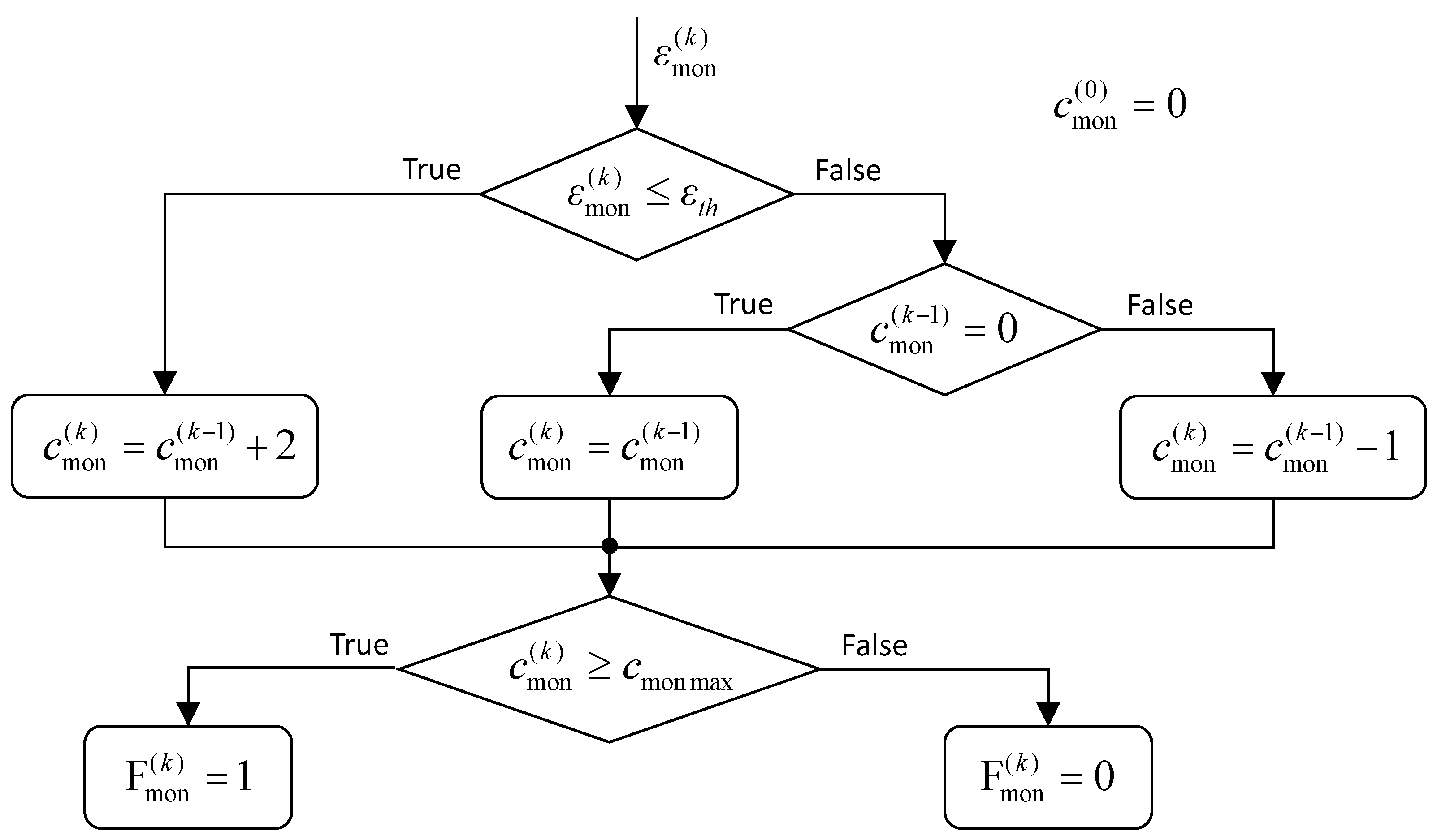
2.4.1. Motion Monitor

The Motion Monitor calculates voted position values for the two motors, and the output shaft, by using triple redundant signals. This is obtained analytically, by combining the measurements of the dual sensors with model-based reconstructions derived from kinematic relationships. In fact, by reformulating Equation (3) in terms of displacements, once that two out of the three quantities θ 1 , θ 2 and x o are known, the resting one can be estimated. Taking into account that the LVDTs provide two linear feedback signals (LF1 and LF2) and that two consolidated angle feedbacks (CAF1 and CAF2, each one obtained by the resolvers related to the i-th motor) are available, five position estimates can be calculated, Equations (5)–(9)
EAF11 = (LF1 − b2 CAF2)/b1,
EAF12 = (LF2 − b2 CAF2)/b1,
EAF21 = (LF1 − b1 CAF1)/b2,
EAF22 = (LF2 − b1 CAF1)/b2,
ELF = b1 CAF1 + b2 CAF2,
The system can thus apply a triple redundancy on each position signal, up to obtain voted output position feedback (VLF) as well as voted angle feedbacks (VAF1 and VAF2), and it is capable of tolerating up to two position sensors faults, except the fault of two resolvers located on different motors, Table 3.

2.4.2. Currents Monitor

The Currents Monitor aims to detect and isolate current sensors faults and motor phases faults, as well as to calculate voted values of phase currents. Also in this case, a model-based technique is used: when a three-phase PMSM correctly operates, the sum of its phase currents is constant (near to zero). From the six current measurements related to the i-th motor (Ix i Y, where x = a, b, c is the motor phase; Y = C, M is the CON or MON sensors set), eight sums of currents can be obtained, Equation (10).
Σ i   =   [ 1 1 1 0 0 0 1 1 0 0 0 1 1 0 0 0 1 1 1 0 1 0 1 0 0 1 0 1 0 1 0 1 1 1 0 0 0 0 1 1 1 0 0 0 0 1 1 1 ] [ I i a C I i b C I i c C I i a M I i b M I i c M ] ,
As reported in Table 4, by selecting the sums of currents (Σi h, with h = 1, …, 8) that contain the same measurement, it is possible to construct six groups (GaC, GbC, GcC, GaM, GbM and GcM). Then, by selecting the groups of sums of currents that also contain the same current data, three classes are obtained (Ca, Cb, Cc).
The algorithm generates the following diagnostic outputs:
  • if all sums of currents do not exceed a predefined threshold, no fault is detected;
  • if the threshold is exceeded by all the sums of currents belonging to a group, a fault of the sensor providing the common measurement is detected;
  • if the threshold is exceeded by all the sums of currents included in a class, a fault of the common coil included in the class is detected.

2.4.3. Jamming Monitor

The Jamming Monitor algorithm is composed of two sections executed in series, dedicated to the fault detection on the motors and the screwshaft, respectively.
In particular, for each k-th monitoring sample (k = 1, 2, …), the algorithm defines a fault flag vector Fmon, in which four Boolean variables identify the occurrence of the four possible jamming events (Fmon|1 and Fmon|2 for the motors jamming, Fmon|ssRJ and Fmon|ssTJ for the screwshaft rotational and translational jamming respectively), Equation (11)
F m o n ( k )   =   [ F mon | 1 ( k ) F mon | 2 ( k ) F mon | ssRJ ( k ) F mon | ssTJ ( k ) ] T ,
If no jamming is detected, all the fault flag vector components are 0 (i.e., false Boolean values). Otherwise, if a jamming is detected, at least one fault flag vector component is 1 (i.e., true Boolean value). The jamming is also isolated if only one vector component is 1.
Each algorithm section uses a generalized Jamming-Detection Logic (JDL), whose flow chart is reported in Figure 3: the fault flag (Fmon) is generated by elaborating a monitor signal (εmon) sampled at the monitoring frequency (fmon). If the monitor signal is lower than a pre-defined threshold (εth), a fault counter (cmon) is increased by 2; if the threshold is exceeded, the fault counter is decreased by 1 if it is positive at the previous step, otherwise it is held at 0. The jamming is detected, when the fault counter exceeds a pre-defined value (cmon max, which basically defines the FDI latency).
In the first section of the algorithm, the jamming related to the i-th motor (i = 1, 2) is targeted. The monitor signal (εmon|i) is defined as the variation of the motor rotation (θi) between two samples, Equation (12),
ε mon | i ( k )   =   | θ i ( k ) θ i ( k 1 ) | ,
{ F mon | i ( k )   =   J D L ( ε mon | i ( k ) )   if | θ i d ( k ) θ i d ( k 1 ) |     ε d i F m o n ( k )   =   0   if | θ i d ( k ) θ i d ( k 1 ) |   <   ε d i ,
and the algorithm operates as follows, Equation (13): if the i-th motor rotation demand (θi d) between two samples varies for more than a pre-defined threshold (εd i), the JDL is executed to define the related fault flag (Fmon|i); otherwise, all fault flags are set to 0 and the system operates normally (AAEP mode). If a motor jamming is detected by the JDL, the related fault flag becomes true and the control laws are reconfigured to engage the appropriate active/stand-by mode (ASB or SBA).
The second section of the algorithm is instead dedicated to the screwshaft jamming FDI, which can result in a rotational or in a translational stuck, due to the jamming of the internal or external screw-nut couplings respectively. A model-based approach is again applied. In normal conditions (AAEP mode), the motors speeds are correlated via Equation (4), while, if there is a screwshaft rotation jamming, the mechanical train imposes that θ ˙ 1   =   p s 2 / p s 1 θ ˙ 2 (given by θ ˙ s s   =   0 in Equation (1)). Otherwise, if the jamming causes a translation stuck, the transmission imposes θ ˙ 1   =   θ ˙ 2 (given by x ˙ s s   =   0 in Equation (2)).
Starting from these considerations, the screwshaft jamming is detected by:
  • reconstructing, via Equation (3), an output speed estimate ( x ˙ o e ) from the motor angle feedbacks, and an output speed demand ( x ˙ o d ) from the motors speed demands;
  • performing a threshold check on an output speed residual ( δ s r ), calculated via Equation (14).
δ s r ( k )   =   | x ˙ o d ( k ) x ˙ o e ( k ) |   =   | b 1 ( θ ˙ 1 d ( k ) θ ˙ 1 ( k ) ) + b 2 ( θ ˙ 2 d ( k ) θ ˙ 2 ( k ) ) | ,
It is worth noting that, if no jamming is occurred, δsr is very small, due to the speed tracking of the EMA control laws, while it is large if there is a jamming. In fact, if we impose the kinematic relationships with or without a screwshaft jamming, the output speed estimate can be approximated via Equation (15) and δsr is given by Equation (16).
x ˙ o e ( k ) { ( b 1 α E P + b 2 ) θ ˙ 2 ( k ) No   jam ( b 1 p s 2 / p s 1 + b 2 ) θ ˙ 2 ( k ) if   θ ˙ s s   =   0 ( b 1 + b 2 ) θ ˙ 2 ( k ) if   x ˙ s s   =   0 ,
δ s r ( k ) { 0 No   jam | b 1 ( α E P p s 2 / p s 1 ) θ ˙ 2 ( k ) + ( b 1 α E P + b 2 ) ( θ ˙ 2 d ( k ) θ ˙ 2 ( k ) ) | if   θ ˙ s s   =   0 | b 1 ( α E P 1 ) θ ˙ 2 ( k ) + ( b 1 α E P + b 2 ) ( θ ˙ 2 d ( k ) θ ˙ 2 ( k ) ) | if   x ˙ s s   =   0 ,
In case of jamming faults, the first contributions at second hands in Equation (16) have large amplitudes (while the second ones are minor, due to motors speed tracking), i.e., any screwshaft jamming implies that δsr is large.
The screwshaft jamming isolation (i.e., rotational or translational stuck) is finally obtained by executing two JDL algorithms in parallel, as summarized by Equations (17) and (18).
{ ε mon | ssRJ ( k )   =   | θ ˙ 1 ( k ) p s 2 / p s 1 θ ˙ 2 ( k ) | ε mon | ssTJ ( k )   =   | θ ˙ 1 ( k ) θ ˙ 2 ( k ) | ,
F m o n ( k ) = { 0 if   δ s r ( k )   <   ε s [ 0 0 J D L ( ε mon | ssRJ ( k ) ) J D L ( ε mon | ssTJ ( k ) ) ] T if   δ s r ( k )     ε s ,
Concerning the parameters of the Jamming Monitor algorithm, they have been defined (Table 5), by taking into account the available computational resources of the ECUs, which have limited the monitoring sampling rate to 2 kHz, and by imposing that the following maxima FDI latencies:
  • 100 ms for the screwshaft jamming faults;
  • 20 ms for the motors jamming, to account for additional delays due to the brake activation and engagement.

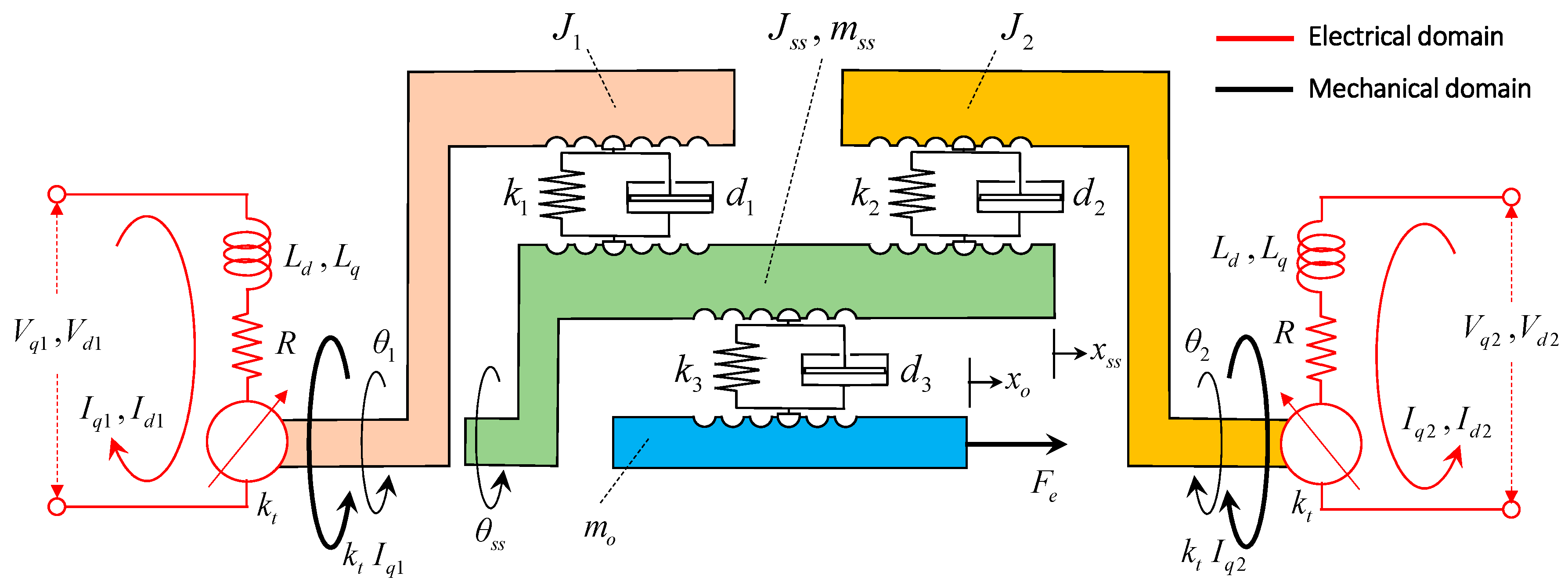
2.5. Nonlinear Dynamic Modelling

As described in Section 2.4, the condition-monitoring algorithms are designed via deterministic model-based approach, by performing threshold checks on monitor signals generated by theoretical predictions of the system behaviour. In practical terms, these predictions can significantly deviate from the actual dynamics (e.g., the sums of the phase currents are not constant, the mechanical train compliance alters the validity of the “rigid” kinematic relationships, the closed-loop bandwidth limitations imply that the motors speed tracking is not ideal), so the FDI effectiveness is generally questionable and it must be verified well before the EMA manufacturing.
The development of a high-fidelity dynamic model and its consequent experimental validation are thus of paramount importance for a deterministic model-based condition-monitoring, especially for the failure transient characterisation. In previous works by the authors [44,45], a preliminary verification of performances were obtained, but the accuracy in terms of motors currents response was poor and the experimental validation was limited to the normal operative condition. Here, an enhanced model of the EMA dynamics is proposed, which has been experimentally validated with reference to all the five operative modes of the EMA (Table 1). The model is composed of:
  • an electromechanical section, simulating
    FOC current dynamics (differently from [44,45], both quadrature and direct currents are simulated);
    5-degree-of-freedom mechanical transmission, with equations of motions related to motors rotation, output translation and screwshaft rotation and translation;
    sliding friction on motors and output shaft described via combined “Coulomb–tanh” model [51,52], with optimized parameters with respect to [44,45];
    mechanical endstrokes (no model was included in [44,45]);
    jamming faults, implying the sudden block of motors rotation, screwshaft rotation or screwshaft translation;
  • an electronic section, including
    sensors errors and nonlinearities (bias, noise, resolution);
    commands nonlinearities (saturation, rate limiting);
    digital signal processing at 2 kHz sampling rate for both monitoring (Table 5) and closed-loop control functions.
As far as the normal operation is concerned (i.e., no faults), the electro-mechanical section of the model, schematically represented by Figure 4, is governed by Equations (19)–(24),
L q I ˙ q   i   =   V q   i     R I q   i     ( k t   +   L d n d I d   i ) θ ˙ i with i   =   1 ,   2 ,
L d I ˙ d   i   =   V d   i     R I d   i   +   L q n d I q   i θ ˙ i with i   =   1 ,   2 ,
J i θ ¨ i   =   k t I q   i     T f r   i tanh ( θ ˙ i ω f r   i )     d i ( θ ˙ i θ ˙ s s 2 π x ˙ s s p s   i )     k i ( θ i θ s s 2 π x s s p s   i )   with   i   =   1 ,   2 ,
J s s θ ¨ s s   =   d 1 ( θ ˙ 1 θ ˙ s s 2 π x ˙ s s p s 1 )   +   k 1 ( θ 1 θ s s 2 π x s s p s 1 ) + d 2 ( θ ˙ 2 θ ˙ s s 2 π x ˙ s s p s 2 )   + +   k 2 ( θ 2 θ s s 2 π x s s p s 2 )     d 3 [ θ ˙ s s + 2 π ( x ˙ s s x ˙ o ) p s 3 ]     k 3 [ θ s s + 2 π ( x s s x o ) p s 3 ] ,
m s s x ¨ s s   =   2 π d 1 p s 1 ( θ ˙ 1 θ ˙ s s 2 π x ˙ s s p s 1 )   +   2 π k 1 p s 1 ( θ 1 θ s s 2 π x s s p s 1 )   +   2 π d 2 p s 2 ( θ ˙ 2 θ ˙ s s 2 π x ˙ s s p s 2 )   + +   2 π k 2 p s 2 ( θ 2 θ s s 2 π x s s p s 2 )     2 π d 3 p s 3 [ θ ˙ s s + 2 π ( x ˙ s s x ˙ o ) p s 3 ]     2 π k 3 p s 3 [ θ s s + 2 π ( x s s x o ) p s 3 ] ,
m o x ¨ o   =   F e     F f r   o tanh ( x ˙ o v f r   o )   +   2 π d 3 p s 3 [ θ ˙ s s + 2 π ( x ˙ s s x ˙ o ) p s 3 ]   +   2 π k 3 p s 3 [ θ s s + 2 π ( x s s x o ) p s 3 ] ,
where Vq i, Vd i, iq i and id i are the quadrature and direct voltages and currents of the i-th motor, Ji and Jss are the motors and the screwshaft inertias, mss and mo are the screwshaft and output shaft masses, R is the motors phase resistance, Ld and Lq are the motors inductances in the rotor frame (which are identical in the reference EMA, because the PMSMs have surface-mounted magnets), kt is the motors torque constant, nd is the number of motors pole pairs, Fe is the external load, km and dm are the stiffness and damping referred to the roto-translating motion deformation of the m-th screw-nut coupling (with m = 1, 2, 3), while Tfr i, ωfr i, Ffr o and vfr o are the parameters of the “Coulomb–tanh” friction models related to the i-th motor and the output shaft, respectively.
Concerning the jamming faults, they are simulated as instantaneous stops of the moving element, as described by Equation (25),
z ˙   = { z ˙ 0   +   0 t z ¨ d t 0     t   <   t f 0 t     t f ; z   = { z 0   +   0 t z ˙ d t 0     t   <   t f z ( t f ) t t f ,
in which z is the position of the element interested by the jamming fault (i.e., z = θ1 or z = θ2 for motors jamming and z = θss or z = xss for screwshaft rotational or translational jamming), tf is the time at which the fault is injected, while z0 and z ˙ 0 are the initial position and speed.
It is worth noting that the proposed model represents a balance between prediction accuracy, objectives of the study and complexity of the model itself. More accurate simulations could include mechanical freeplay [30], sophisticated friction models [51,52] and iron losses in the motor [53,54], but the inclusion of these model features would entail minor effects for the examined application. In particular, the mechanical freeplay, due to the screw-nut couplings preload, was extremely small in the reference EMA and its contribution in the model would have been poor. Similarly, the motor iron losses have been neglected because they depend on electrical frequency, which is relatively small for the reference EMA (<60 Hz, Table 6) and their impact on actuator dynamics in the positiontracking frequency range (<20 Hz) is expected to be minor. On the other hand, more accurate friction models (including load and temperature dependence) could significantly enhance the simulation, but a simplified approach has been preferred for both the lack of detailed information and to limit the number of model parameters.
The EMA model has been developed in the Matlab–Simulink–Stateflow environment and the numerical simulation is solved by the Runge–Kutta method, with 10−5 s integration step. It is worth noting that the choice of a fixed-step solver is not strictly related to the objectives of this work, in which the model (once experimentally validated) is used for “off-line” simulations testing the FDI algorithms, but it has been selected for the next steps of the project, when the FDI system will be implemented in the ECU boards via automatic Matlab compiler and executed in “real-time”.
The parameters of the electro-mechanical section of the model are given in Table 6.

2.6. ECU Prototype for Experimental Tests

Since one of the main objectives of the research was to assess the FDI capabilities of the condition-monitoring system in case of mechanical jamming or motors faults before the final design of the dual CON-MON ECUs, an intermediate step has been made, by developing a prototype simplex ECU.
In the prototype ECU (whose block diagram is reported in Figure 5), the condition-monitoring algorithms and the redundancy management functions are not implemented, but the fault-tolerant closed-loop control is the same of the final design.
Considering that, as outlined in Table 1, the relationship between the output shaft speed and the motors speeds varies with the operative mode, some kind of reconfiguration technique must be implemented to assure the system stability and the dynamic performances in all modes. In the proposed design, based on three nested loops, on motors currents, motors speeds and output shaft position,
  • all the regulators implement proportional/integral actions on tracking error signals, plus anti-windup function with back-calculation algorithm [55] to compensate for commands saturation;
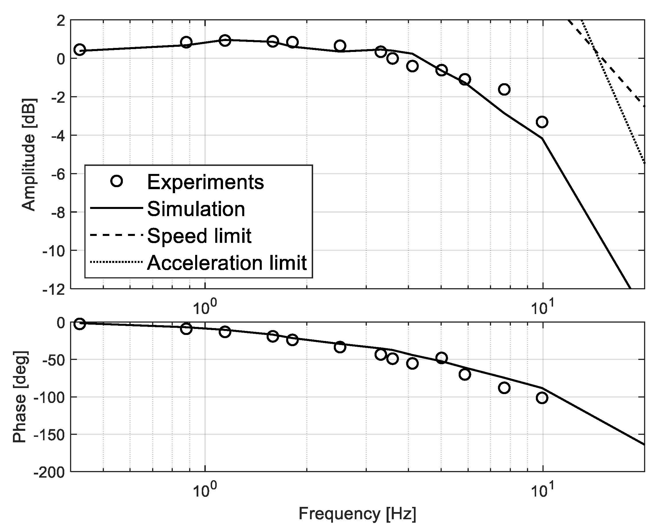
  • the innermost loops on motors currents and motors speeds are processed at 2 kHz and use fixed parameters (i.e., they don’t vary with EMA mode). They provide tracking bandwidths of 420 Hz and 58 Hz, on currents and speeds, respectively;
  • the reconfiguration strategy is applied to the outermost loop only, which is processed at 1 kHz (due to a prototype ECU limitation) and it can be reconfigured through a dedicated mode switching signal.
In the dual CON-MON ECUs, the mode switch comes from the condition-monitoring algorithms, while in the prototype ECU it is imposed by the operator via the test rig, together with the EMA position demand (Figure 5).
Thanks to this prototype ECU, the system dynamic performances have been characterized in both frequency and time domains for each operative mode, aiming to validate the simulation results provided by the EMA model and to permit the design of the condition-monitoring algorithms via model-based approach.

3. Results and Discussion

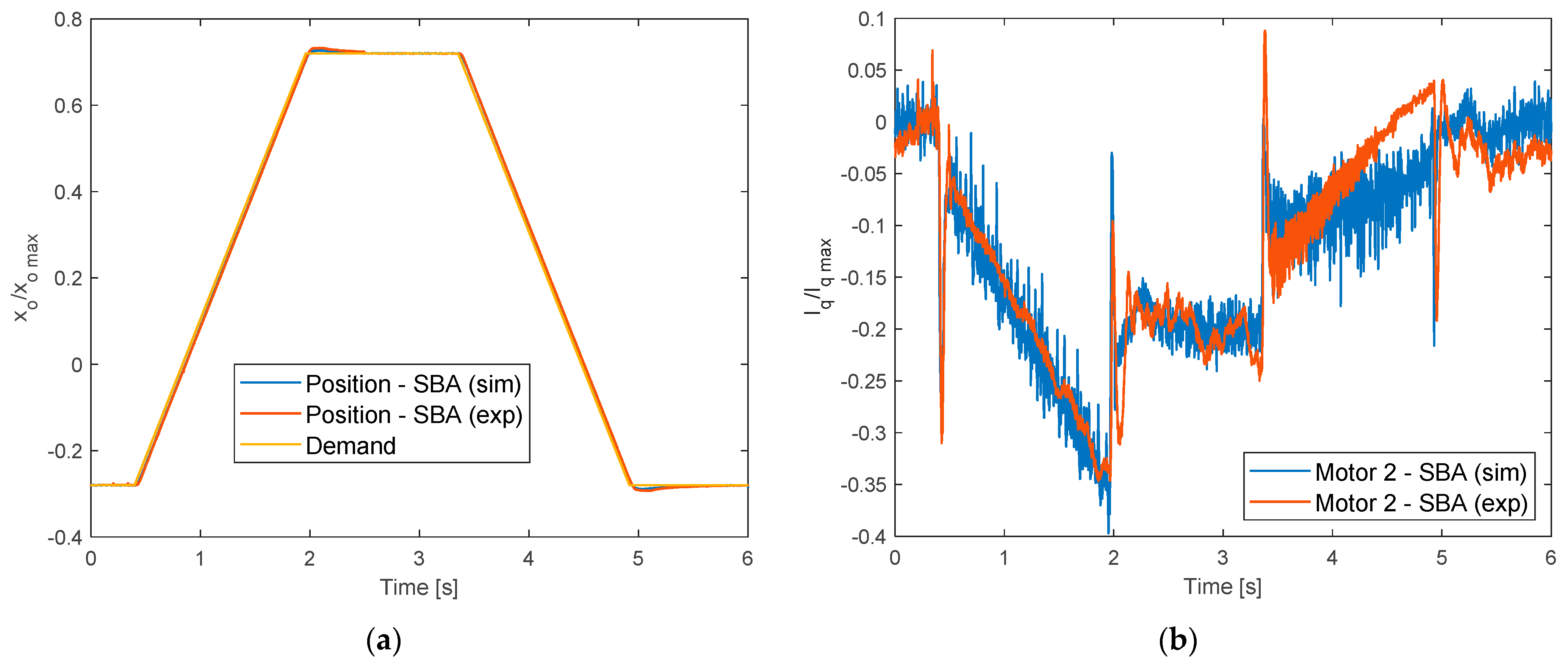
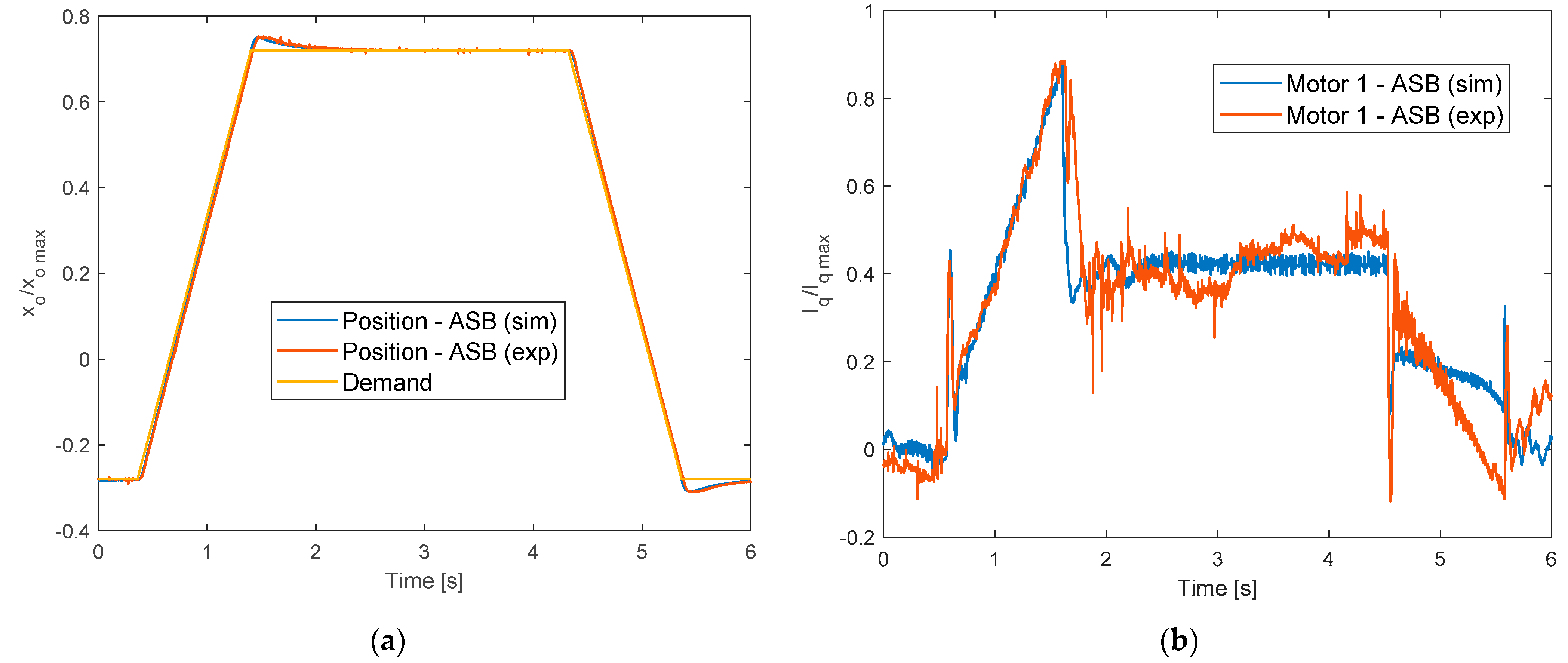
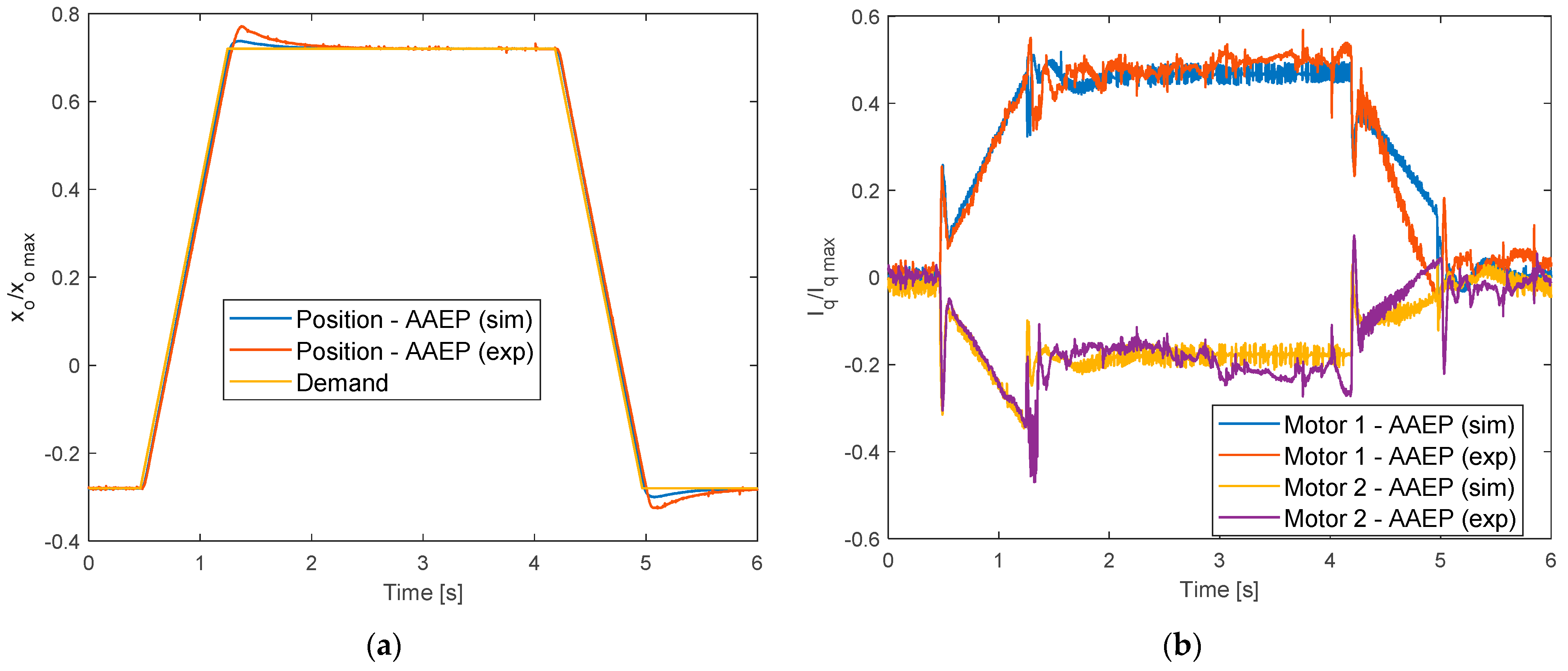
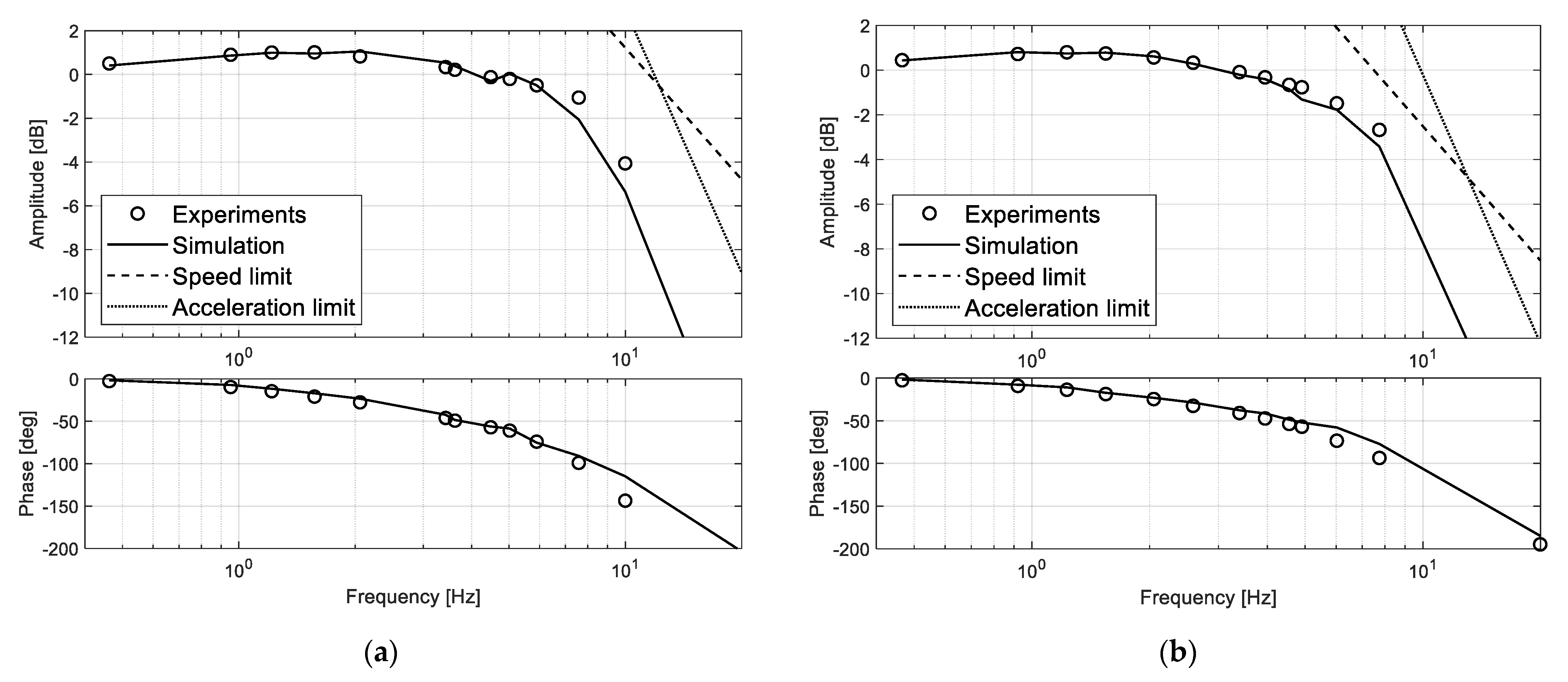
3.1. Experimental Validation of the Model

Excerpts of the model validation results are reported from Figure 6, Figure 7, Figure 8, Figure 9, Figure 10 and Figure 11.
The most relevant time-domain responses are reported from Figure 6, Figure 7 and Figure 8, with reference to both active/stand-by modes and the normal operation (AAEP mode), by focusing the attention on position and currents dynamics. All the time-domain responses are referred to position tracking tests in which the EMA is commanded to follow a large-amplitude rate-limited square-wave signal under 100 kN/m spring-type load, which is roughly representative of the worst-case flight conditions. More precisely, by referring to Equation (24), the test have been carried out by imposing
F e   =   k e ( x o   +   x o   max 4 ) ,
where ke = 105 N/m and xo max = 0.025 m. Thus, from Figure 6, Figure 7 and Figure 8, the external load is opposite to (aiding) the EMA motion when the output speed is positive (negative).
Satisfactory results are generally obtained, with concrete enhancement of the motor currents predictions with respect to [44,45]. In SBA mode, the currents prediction is accurate in both steady-state and transient phases, with overall accuracy of 2 A, Figure 6b. The predictions in terms of position response are more accurate (it is expected since the signal is characterised by a low-frequency content), with errors lower than 0.15 mm (0.3% of the EMA full stroke), Figure 6a. In ASB mode, the errors on currents simulation during steady-state conditions are limited to 2 A (i.e., 8% of the maximum current), but the errors tend to increase at the abrupt transients derived from command signal variations and when the EMA performs a dynamic position tracking with aiding load, Figure 7b. This behaviour essentially depends on the simplified friction model used for the EMA simulation: a load-dependant model could probably enhance the results and further developments of the research will take into account this point. Concerning the position response, it anyway exhibits a good accuracy, with errors lower than 0.25 mm (0.5% of the EMA full stroke). It is also worth noting that both simulation and experiment point out that the position response is characterised by a slight overshoot (0.75 mm), related to a too moderate anti-windup action in the position regulator, Figure 7a. Similar results characterise the simulation in AAEP mode (Figure 8), even if the prediction errors on position response increase during the overshoot phase, by reaching 0.8 mm (1.6% of the EMA full stroke).
Excerpts of results of the frequency-domain validation of the model are then reported from Figure 9, Figure 10 and Figure 11, in which the position tracking responses to sinusoidal demand waves of 0.5 mm (i.e., 1% of the EMA full stroke) under a 2 kN compressive load are proposed in terms of amplitude and phase of the first harmonic signal component. The plots also report the speed and acceleration limits of the EMA and it can be verified that, in the examined frequency range and for all operative modes, the system works without encountering saturation phenomena.
The frequency responses highlight that the model is very accurate for small-displacement dynamics (relevant for flight control applications): for input frequencies up to 10 Hz, the prediction errors are actually comparable to sensors accuracy (i.e., 0.1% of the EMA full stroke).

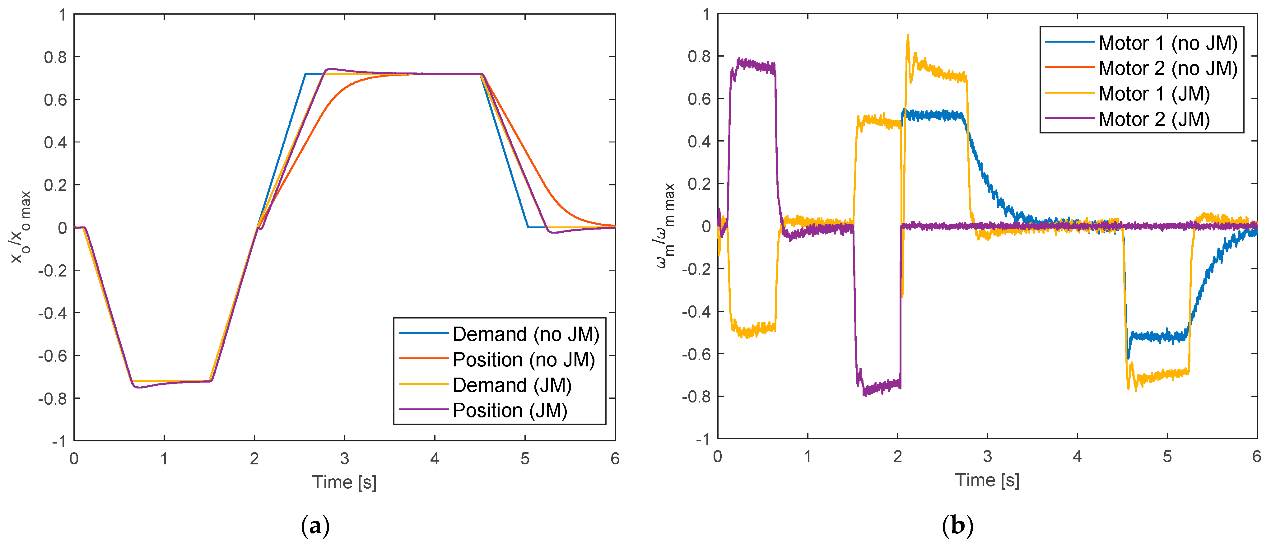
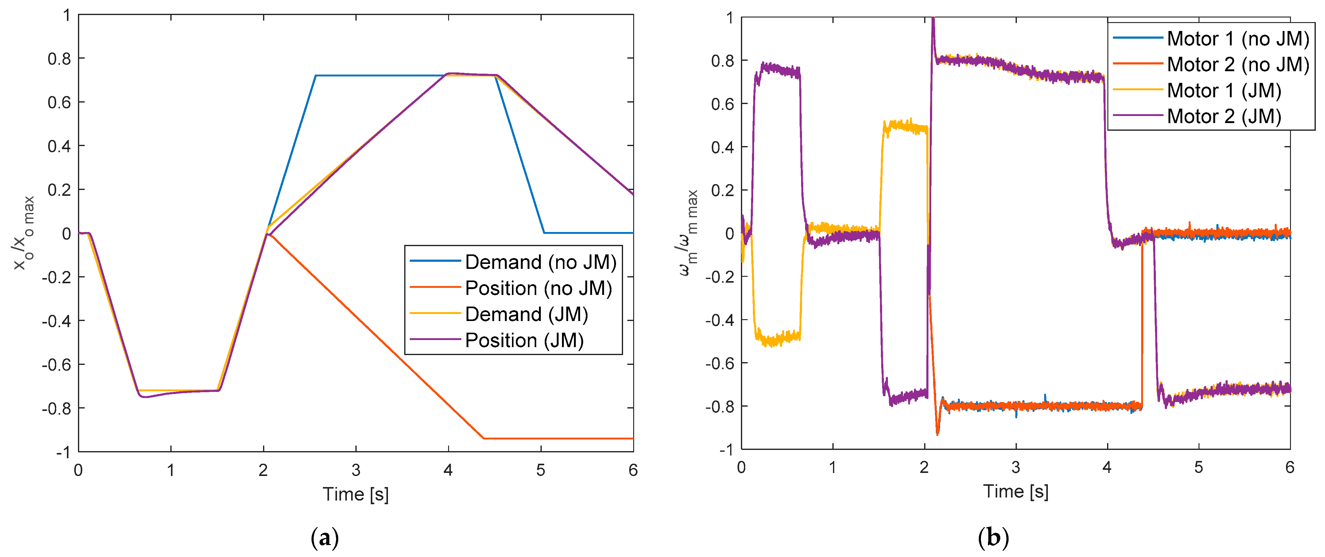
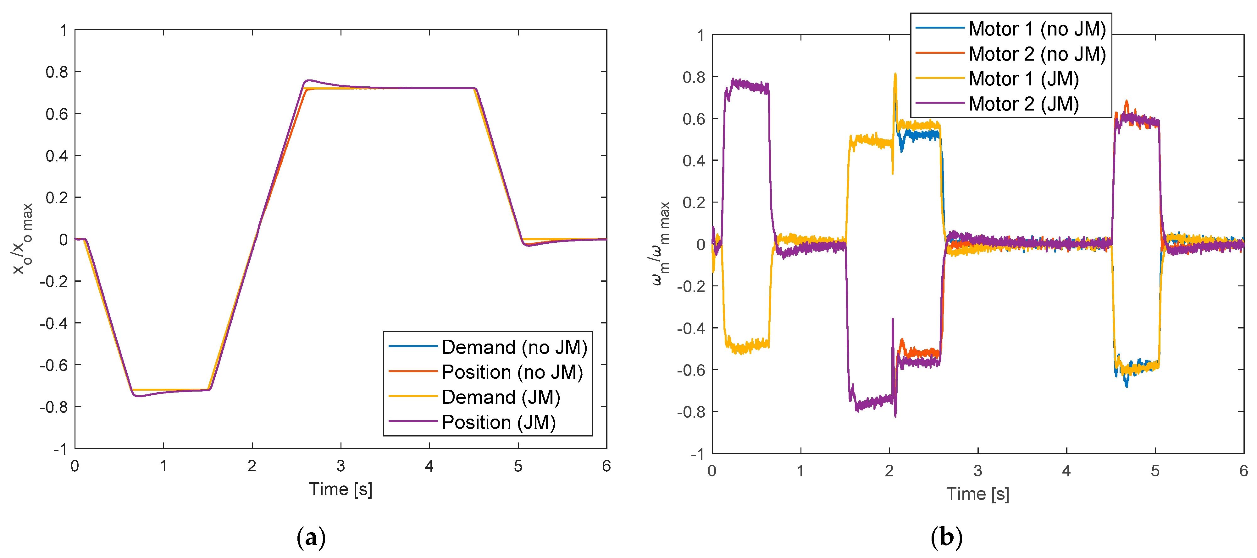
3.2. Jamming Failure Transient Characterisation

The validated model is then used to verify the condition-monitoring performances, by injecting the jamming faults in different points of the mechanical train and by evaluating the FDI latency to implement the correct operative mode switching and the control laws reconfiguration. The most relevant results are reported from Figure 12, Figure 13 and Figure 14 and are related to the motor 2 jamming and to the screwshaft jamming respectively. To evaluate the effectiveness of the Jamming Monitor (JM), the responses in terms of output position and motors speeds are reported with and without the JM execution.
All the simulations are carried out by commanding the EMA, under 2.4 kN compressive load, to track a large-displacement demand (±18 mm, i.e., 75% of the EMA full stroke) at maximum speed and by simulating a jamming when the actuator reaches its midstroke (i.e., at 2.03 s).
The simulation points out that in case of motor 2 jamming, causing the operation to switch from AAEP to ASB mode (Figure 12), the FDI latency is extremely small (10 ms, similar to the one obtained in [44,45]), but immediately after the fault compensation the EMA tends to diverge from the correct position tracking, Figure 12a. This behaviour results from an imperfect reconfiguration of the position regulator (related to integral operator initialization), which implies a reverse speed demand to the active motor, Figure 12b.
The failure transient related to the screwshaft translational jamming, causing the operation to switch from AAEP to AAPR mode (Figure 13), is effectively minimized by the JM (FDI latency is 15 ms, larger than the one obtained in [44,45]), even if the EMA dynamic performances after the fault are significantly reduced (as also confirmed by Figure 10a). The faulty dynamics without JM is dramatically negative, since the EMA reacts to the jamming by oppositely diverging with respect to the position demand and it rapidly reaches the endstroke, Figure 13a. It is worth noting that the model enhancement has permitted to correctly reproduce this critical behaviour, by including the simulation of the impact on mechanical endstrokes.
Finally, the results related to the screwshaft rotational jamming, causing the operation to switch from AAEP to AAPT mode (Figure 14), point out that the FDI latency is more concrete (90 ms, again larger than the one obtained in [44,45]), but no relevant variation in tracking performances is observable after the fault (Figure 14a), because the reconfiguration of motors speeds demands generated by the fault-tolerant control laws are very close to the ones before the fault, Figure 14b.

4. Conclusions

A condition-monitoring system for the detection and isolation of faults in a fault-tolerant EMA for flight control applications is developed via deterministic model-based approach. The monitoring algorithms are designed and verified by using a detailed nonlinear model of the EMA, which simulates, by physical first-principles, the most relevant phenomena involved in the system dynamics (structural compliance of the mechanical train, field-oriented control of the motors currents, sliding friction, digital signal processing, sensors errors, major faults). The model is experimentally validated in both time and frequency domains for normal operative conditions and with jamming faults. The results demonstrate that the EMA is capable of operating after a mechanical jamming. A particular attention is paid to the failure transient characterisation (strongly relevant for aircraft applications), pointing out that the monitoring algorithms, composed of two sections dedicated to the blocks of motors and differential screws, respectively, succeed in detecting and isolating the fault at different locations of the mechanical transmission, with fault latency lower than 90 ms.

Author Contributions

Methodology, investigation and writing—original draft preparation, G.D.R. and B.L.; writing—review and editing and formal analysis, G.D.R.; software and data curation, B.L.; validation and resources, G.D.R., B.L., N.B., M.N.; conceptualization, visualization and supervision, N.B. and M.N. All authors have read and agreed to the published version of the manuscript.

Funding

This research received no external funding.

Institutional Review Board Statement

Not applicable.

Informed Consent Statement

Not applicable.

Conflicts of Interest

The authors declare no conflict of interest.

References

  1. Flightpath 2050: Europe’s Vision for Aviation. Available online: https://op.europa.eu/en/publication-detail/-/publication/7d834950-1f5e-480f-ab70-ab96e4a0a0ad/language-en (accessed on 25 August 2021).
  2. Schäfer, A.W.; Barrett, S.R.H.; Doyme, K.; Dray, L.; Gnadt, A.R.; Self, R.; O’Sullivan, A.; Synodinos, A.; Torija, A.J. Technological, economic and environmental prospects of all-electric aircraft. Nat. Energy 2019, 4, 160–166. [Google Scholar] [CrossRef] [Green Version]
  3. Howse, M. All-electric aircraft. Power Eng. J. 2003, 17, 35–37. [Google Scholar] [CrossRef]
  4. Rosero, J.A.; Ortega, J.A.; Aldabas, E.; Romeral, L. Moving towards a more electric aircraft. IEEE Aerosp. Electron. Syst. Mag. 2007, 22, 3–9. [Google Scholar] [CrossRef] [Green Version]
  5. Roboam, X.; Sareni, B.; De Andrade, A. More Electricity in the Air: Toward Optimized Electrical Networks Embedded in More-Electrical Aircraft. IEEE Ind. Electron. Mag. 2012, 6, 6–17. [Google Scholar] [CrossRef] [Green Version]
  6. Madonna, V.; Giangrande, P.; Galea, M. Electrical Power Generation in Aircraft: Review, Challenges, and Opportunities. IEEE Trans. Transp. Electrif. 2018, 4, 646–659. [Google Scholar] [CrossRef]
  7. Botten, S.L.; Whitley, C.R.; King, A.D. Flight Control Actuation Technology for Next-Generation All-Electric Aircraft. Technol. Rev. J. 2000, 8, 55–68. [Google Scholar]
  8. Maré, J.-C.; Fu, J. Review on signal-by-wire and power-by-wire actuation for more electric aircraft. Chin. J. Aeronaut. 2017, 30, 857–870. [Google Scholar] [CrossRef]
  9. Mazzoleni, M.; Di Rito, G.; Previdi, F. Introduction. In Electro-Mechanical Actuators for the More Electric Aircraft; Advances in Industrial Control; Springer: Cham, Switzerland, 2021; Volume 2, pp. 1–44. [Google Scholar] [CrossRef]
  10. Jensen, S.C.; Jenney, G.D.; Dawson, D. Flight test experience with an electromechanical actuator on the F-18 Systems Research Aircraft. In Proceedings of the 19th Digital Avionics Systems Conference, Philadelphia, PA, USA, 7–13 October 2000; Volume 1, pp. 2E3/1–2E3/10. [Google Scholar] [CrossRef]
  11. Maré, J.-C. Aerospace Actuators—Volume 2: Signal-by-Wire and Power-by-Wire; Bourrières, J.-P., Ed.; ISTE Ltd.: Washington, DC, USA; John Wiley & Sons: Hoboken, NJ, USA, 2017; pp. 171–217. [Google Scholar] [CrossRef]
  12. Di Rito, G.; Galatolo, R.; Schettini, F. Experimental and simulation study of the dynamics of an electro-mechanical landing gear actuator. In Proceedings of the 30th Congress of the International Council of the Aeronautical Sciences (ICAS), Daejeon, Korea, 25–30 September 2016. [Google Scholar]
  13. Giangrande, P.; Al-Timimy, A.; Galassini, A.; Papadopoulos, S.; Degano, M.; Galea, M. Design of PMSM for EMA employed in secondary flight control systems. In Proceedings of the 2018 IEEE International Conference on Electrical Systems for Aircraft, Railway, Ship Propulsion and Road Vehicles & International Transportation Electrification Conference (ESARS-ITEC), Nottingham, UK, 7–9 November 2018; pp. 1–6. [Google Scholar] [CrossRef]
  14. Qiao, G.; Liu, G.; Shi, Z.; Wang, Y.; Ma, S.; Lim, T.C. A review of electromechanical actuators for More/All Electric aircraft systems. Proc. Inst. Mech. Eng. Part C J. Mech. Eng. Sci. 2018, 232, 4128–4151. [Google Scholar] [CrossRef] [Green Version]
  15. Mazzoleni, M.; Di Rito, G.; Previdi, F. Reliability and safety of electro-mechanical actuators for aircraft applications. In Electro-Mechanical Actuators for the More Electric Aircraft; Advances in Industrial Control; Springer: Cham, Switzerland, 2021; Volume 2, pp. 45–85. [Google Scholar] [CrossRef]
  16. Balaban, E.; Bansal, P.; Stoelting, P.; Saxena, A.; Goebel, K.F.; Curran, S. A diagnostic approach for electro-mechanical actuators in aerospace systems. In Proceedings of the 2009 IEEE Aerospace Conference, Big Sky, MT, USA, 7–14 March 2009; pp. 1–13. [Google Scholar] [CrossRef]
  17. Ossmann, D.; Van der Linden, F.-L.-J. Advanced sensor fault detection and isolation for electro-mechanical flight actuators. In Proceedings of the NASA/ESA Conference on Adaptive Hardware and Systems, Montreal, QC, Canada, 15–18 June 2015; pp. 1–8. [Google Scholar]
  18. Ismail, M.A.A.; Balaban, E.; Spangenberg, H. Fault detection and classification for flight control electromechanical actuators. In Proceedings of the 2016 IEEE Aerospace Conference, Big Sky, MT, USA, 5–12 March 2016; pp. 1–10. [Google Scholar] [CrossRef]
  19. Ismail, M.A.A.; Windelberg, J. Fault detection of bearing defects for ballscrew based electro-mechanical actuators. In Proceedings of the World Congress on Condition Monitoring (WCCM), London, UK, 13–16 June 2017; pp. 1–12. [Google Scholar]
  20. Smith, M.J.; Byington, C.S.; Watson, M.J.; Bharadwaj, S.; Swerdon, G.; Goebel, K.; Balaban, E. Experimental and analytical development of health management for electro-mechanical actuators. In Proceedings of the 2009 IEEE Aerospace conference, Big Sky, MT, USA, 7–14 March 2009; pp. 1–14. [Google Scholar] [CrossRef]
  21. Garcia, J.R.; Cusido, J.; Rosero, J.A.; Ortega, J.A.; Romeral, L. Reliable electro-mechanical actuators in aircraft. IEEE Aerosp. Electron. Syst. Mag. 2008, 23, 19–25. [Google Scholar] [CrossRef]
  22. Bennett, J.; Mecrow, B.; Atkinson, D. Safety-critical design of electromechanical actuation systems in commercial aircraft. IET Electr. Power Appl. 2011, 5, 37–47. [Google Scholar] [CrossRef]
  23. Bennett, J.W.; Atkinson, G.J.; Mecrow, B.C.; Atkinson, D.J. Fault-Tolerant Design Considerations and Control Strategies for Aerospace Drives. IEEE Trans. Ind. Electron. 2011, 59, 2049–2058. [Google Scholar] [CrossRef]
  24. Rottach, M.; Gerada, C.; Wheeler, P.-W. Design optimisation of a fault-tolerant PM motor drive for an aerospace actuation application. In Proceedings of the 7th IET International Conference on Power Electronics, Machines and Drives (PEMD), Manchester, UK, 8–10 April 2014; pp. 1–6. [Google Scholar] [CrossRef]
  25. Arriola, D.; Thielecke, F. Design of fault-tolerant control functions for a primary flight control system with electromechanical actuators. In Proceedings of the International Automatic Testing Conference, AUTOTESTCON, National Harbour, MD, USA, 2–5 November 2015; pp. 393–402. [Google Scholar] [CrossRef]
  26. Di Rito, G.; Galatolo, R.; Schettini, F. Self-monitoring electro-mechanical actuator for medium altitude long endurance unmanned aerial vehicle flight controls. Adv. Mech. Eng. 2016, 8, 1–12. [Google Scholar] [CrossRef] [Green Version]
  27. Byington, C.; Sloelting, P.; Watson, M.; Edwards, D. A model-based approach to prognostics and health management for flight control actuators. In Proceedings of the 2004 IEEE Aerospace Conference, Big Sky, MT, USA, 6–13 March 2004; pp. 3551–3562. [Google Scholar] [CrossRef]
  28. Mazzoleni, M.; Maccarana, Y.; Previdi, F.; Pispola, G.; Nardi, M.; Perni, F.; Toro, S. Development of a reliable electro-mechanical actuator for primary control surfaces in small aircrafts. In Proceedings of the 2017 IEEE International Conference on Advanced Intelligent Mechatronics (AIM), Munich, Germany, 3–7 July 2017; pp. 1142–1147. [Google Scholar] [CrossRef]
  29. Mazzoleni, M.; Previdi, F.; Scandella, M.; Pispola, G. Experimental Development of a Health Monitoring Method for Electro-Mechanical Actuators of Flight Control Primary Surfaces in More Electric Aircrafts. IEEE Access 2019, 7, 153618–153634. [Google Scholar] [CrossRef]
  30. Di Rito, G.; Schettini, F.; Galatolo, R. Model-based prognostic health-management algorithms for the freeplay identification in electromechanical flight control actuators. In Proceedings of the 2018 IEEE International Workshop on Metrology for AeroSpace, Rome, Italy, 20–22 June 2018; pp. 340–345. [Google Scholar] [CrossRef]
  31. Todeschi, M.; Baxerres, L. Health Monitoring for the Flight Control EMAs. IFAC-PapersOnLine 2015, 48, 186–193. [Google Scholar] [CrossRef]
  32. Blanke, M.; Kinnaert, M.; Lunze, J.; Staroswiecki, M.; Schröder, J. Diagnosis and Fault-Tolerant Control; Springer: Berlin/Heidelberg, Germany, 2016. [Google Scholar] [CrossRef] [Green Version]
  33. Di Rito, G.; Schettini, F. Health monitoring of electromechanical flight actuators via position-tracking predictive models. Adv. Mech. Eng. 2018, 10, 1–12. [Google Scholar] [CrossRef]
  34. Ferranti, L.; Wan, Y.; Keviczky, T. Fault-tolerant reference generation for model predictive control with active diagnosis of elevator jamming faults. Int. J. Robust Nonlinear Control 2018, 29, 5412–5428. [Google Scholar] [CrossRef]
  35. Ferranti, L.; Wan, Y.; Keviczky, T. Predictive flight control with active diagnosis and reconfiguration for actuator jamming. IFAC-PapersOnLine 2015, 48, 166–171. [Google Scholar] [CrossRef]
  36. Arriola, D.; Thielecke, F. Model-based design and experimental verification of a monitoring concept for an active-active electromechanical aileron actuation system. Mech. Syst. Signal Process. 2017, 94, 322–345. [Google Scholar] [CrossRef]
  37. Annaz, F.Y. Fundamental design concepts in multi-lane smart electromechanical actuators. Smart Mater. Struct. 2005, 14, 1227–1238. [Google Scholar] [CrossRef]
  38. Yu, Z.Y.; Niu, T.; Dong, H.L. A jam-tolerant electromechanical system. In Proceedings of the ACTUATOR 2018: 16th International Conference on New Actuators, Bremen, Germany, 25–27 June 2018; pp. 551–554. [Google Scholar]
  39. Gao, Z.; Cecati, C.; Ding, S.X. A Survey of Fault Diagnosis and Fault-Tolerant Techniques—Part I: Fault Diagnosis with Model-Based and Signal-Based Approaches. IEEE Trans. Ind. Electron. 2015, 62, 3757–3767. [Google Scholar] [CrossRef] [Green Version]
  40. Gao, Z.; Cecati, C.; Ding, S.X. A Survey of Fault Diagnosis and Fault-Tolerant Techniques—Part II: Fault Diagnosis with Knowledge-Based and Hybrid/Active Approaches. IEEE Trans. Ind. Electron. 2015, 62, 3768–3774. [Google Scholar] [CrossRef] [Green Version]
  41. Mazzoleni, M.; Di Rito, G.; Previdi, F. Fault diagnosis and condition monitoring approaches. In Electro-Mechanical Actuators for the More Electric Aircraft; Advances in Industrial Control; Springer: Cham, Switzerland, 2021; Volume 3, pp. 87–117. [Google Scholar] [CrossRef]
  42. Chirico, A.J.; Kolodziej, J.R. A Data-Driven Methodology for Fault Detection in Electromechanical Actuators. J. Dyn. Syst. Meas. Control 2014, 136, 041025. [Google Scholar] [CrossRef]
  43. Bodden, D.S.; Clements, N.S.; Schley, B.; Jenney, G. Seeded failure testing and analysis of an electro-mechanical actuator. In Proceedings of the 2007 IEEE Aerospace Conference, Big Sky, MT, USA, 7–14 March 2007; pp. 1–8. [Google Scholar] [CrossRef]
  44. Di Rito, G.; Luciano, B.; Borgarelli, N.; Nardeschi, M. Health-monitoring of a jamming-tolerant electro-mechanical actuator with differential ball screws. In Proceedings of the 2020 IEEE International Workshop on Metrology for Aerospace, Pisa, Italy, 22–24 June 2020; pp. 84–89. [Google Scholar] [CrossRef]
  45. Mazzoleni, M.; Di Rito, G.; Previdi, F. Fault diagnosis and condition monitoring of aircraft electro-mechanical actuators. In Electro-Mechanical Actuators for the More Electric Aircraft; Advances in Industrial Control; Springer: Cham, Switzerland, 2021; Volume 4, pp. 119–224. [Google Scholar] [CrossRef]
  46. Texas Instruments. C2000 Real-Time Microcontrollers. Available online: https://www.ti.com/product/TMS320F28335 (accessed on 25 August 2021).
  47. Allegro Microsystems. Automotive Grade, Fully Integrated, Hall-Effect-Based Linear Current Sensor IC with 2.1 kVRMS Voltage Isolation and Low-Resistance Current Conductor. Available online: https://www.allegromicro.com/en/products/sense (accessed on 25 August 2021).
  48. Tamagawa. Brushless Resolvers (Smartsyn). Available online: https://www.tamagawa-seiki.com/products/resolver-synchro/brushless-resolver-smartsyn.html (accessed on 25 August 2021).
  49. Analog Devices. AD2S1210 Variable Resolution, 10-Bit to 16-Bit R/D Converter with Reference Oscillator. Available online: https://www.analog.com/en/products/ad2s1210.html (accessed on 25 August 2021).
  50. Meggitt. DJD100759C0 LVDT Simplex ±37 mm. Available online: https://www.meggittsensorex.fr/en/sensorex-catalog/technologies/lvdt/ (accessed on 25 August 2021).
  51. Olsson, H.; Åström, K.; De Wit, C.C.; Gäfvert, M.; Lischinsky, P. Friction Models and Friction Compensation. Eur. J. Control 1998, 4, 176–195. [Google Scholar] [CrossRef] [Green Version]
  52. Andersson, S.; Söderberg, A.; Björklund, S. Friction models for sliding dry, boundary and mixed lubricated contacts. Tribol. Int. 2007, 40, 580–587. [Google Scholar] [CrossRef]
  53. Dutta, C.; Tripathi, S.M. Comparison between conventional and loss d-q model of PMSM. In Proceedings of the International Conference on Emerging Trends in Electrical Electronics & Sustainable Energy Systems (ICETEESES), Sultanpur, India, 11–12 March 2016; pp. 256–260. [Google Scholar] [CrossRef]
  54. Zhang, C.; Tian, Z.; Dong, Y.; Zhang, S. Analysis of losses and thermal model in a surface-mounted permanent-magnet synchronous machine over a wide-voltage range of rated output power operation. In Proceedings of the IEEE Conference and Expo Transportation Electrification Asia-Pacific (ITEC Asia-Pacific), Beijing, China, 31 August–3 September 2014; pp. 1–5. [Google Scholar] [CrossRef]
  55. Åström, K.J.; Hägglund, T. Advanced PID Control; ISA—The Instrumentation, Systems, and Automation Society: Pittsburgh, PA, USA, 2006. [Google Scholar]
Figure 1. Fault-tolerant EMA by Umbragroup: (a) prototype on the test rig; (b) patented kinematic concept.
Actuators 10 00230 g001
Figure 2. Block diagram representing the data exchange among the dual CON-MON ECUs.
Actuators 10 00230 g002
Figure 3. Flow chart of the generalized Jamming Detection Logic (JDL).
Actuators 10 00230 g003
Figure 4. Schematics of the electro-mechanical section of the model.
Actuators 10 00230 g004
Figure 5. Simplex ECU prototype for the experimental validation of the EMA model.
Actuators 10 00230 g005
Figure 6. Time-domain model validation: position tracking in SBA mode with 100 kN/m spring-type loading (in Equation (24), ke = 105 N/m); (a) output position; (b) motors quadrature currents (xo max = 25 × 10−3 m; Iq max = 25 A).
Actuators 10 00230 g006
Figure 7. Time-domain model validation: position tracking in ASB mode with 100 kN/m spring-type loading (in Equation (24), ke = 105 N/m); (a) output position; (b) motors quadrature currents (xo max = 25 × 10−3 m; Iq max = 25 A).
Actuators 10 00230 g007
Figure 8. Time-domain model validation: position tracking in AAEP mode with 100 kN/m spring-type loading (in Equation (24), ke = 105 N/m); (a) output position; (b) motors quadrature currents (xo max = 25 × 10−3 m; Iq max = 25 A).
Actuators 10 00230 g008
Figure 9. Frequency-domain model validation: position tracking at 1% maximum demand amplitude (0.5 mm), with 2 kN compressive load; (a) ASB mode; (b) SBA mode.
Actuators 10 00230 g009
Figure 10. Frequency-domain model validation: position tracking at 1% maximum demand amplitude (0.5 mm), with 2 kN compressive load; (a) AAPR mode; (b) AAPT mode.
Actuators 10 00230 g010
Figure 11. Frequency-domain model validation in AAEP mode: position tracking at 1% maximum demand amplitude (0.5 mm), with 2 kN compressive load.
Actuators 10 00230 g011
Figure 12. Jamming Monitor (JM) effect with block of motor 2 at 2.03 s (FDI latency = 10 ms): (a) output position; (b) motors speeds.
Actuators 10 00230 g012
Figure 13. Jamming Monitor (JM) effect with block of screwshaft translation (jamming of the external screw-nut coupling) at 2.03 s (FDI latency = 15 ms): (a) output position; (b) motors speeds.
Actuators 10 00230 g013
Figure 14. Jamming Monitor (JM) effect with block of screwshaft rotation (jamming of the internal screw-nut coupling) at 2.03 s (FDI latency = 90 ms); (a) output position; (b) motors speeds.
Actuators 10 00230 g014
Table 1. Fault-tolerant EMA operative modes.
ModeMotor 1
State
Motor 2
State
Screwshaft
Motion
Motors Speeds
Constraint
Output Speed
ASB
(fail-operative)
ActiveBraked &
De-energized
Roto-translation θ ˙ 2   =   0 b 1 θ ˙ 1
SBA
(fail-operative)
Braked &
De-energized
ActiveRoto-translation θ ˙ 1   =   0 b 2 θ ˙ 2
AAPT
(fail-operative)
ActiveActiveTranslation θ ˙ 1   =   p s 2 / p s 1 θ ˙ 2 ( b 1 p s 2 / p s 1 + b 2 ) θ ˙ 2
AAPR
(fail-operative)
ActiveActiveRotation θ ˙ 1   =   θ ˙ 2 ( b 1 + b 2 ) θ ˙ 2
AAEP
(normal operation)
ActiveActiveRoto-translation θ ˙ 1   =   α E P θ ˙ 2 ( b 1 α E P + b 2 ) θ ˙ 2
Table 2. EMA control sensors data [47,48,49,50].
ComponentModelRangeAccuracy
Current sensorAllegro ACS714±30 A0.3 A
ResolverTamagawa TS2651N141E78±π rad0.0029 rad
Resolver analog-to-digital converterAnalog Devices AD2S1210±π rad0.0014 rad
LVDTMeggitt DJD100759C0±0.037 m5 × 10−5 m
Table 3. Motion Monitor: EMA operative states resulting from position sensors faults.
n. of Sensor FaultsCAF1CAF2LF1LF2VAF1VAF2VLFEMA State
0OKOKOKOKCAF1CAF2LF1OK
EAF11EAF21LF2
EAF12EAF22ELF
1FailOKOKOKEAF11CAF2LF1OK
EAF12LF2
OKFailOKOKCAF1CAF2LF1
EAF22LF2
OKOKFailOKCAF1CAF2LF2
EAF12EAF22ELF
OKOKOKFailCAF1CAF2LF1
EAF11EAF21ELF
2FailOKFailOKEAF12CAF2LF2OK
FailOKOKFailEAF11CAF2LF1OK
OKFailFailOKCAF1EAF22LF2OK
OKFailOKFailCAF1EAF21LF1OK
OKOKFailFailCAF1CAF2ELFOK
FailFailOKOKNo signalNo signalLF1Fail
LF2
Table 4. Currents Monitor: groups and classes for FDI of sensors and coil faults to the i-th motor.
GroupSums of CurrentsCommon MeasurementClass
GaCΣi1, Σi2, Σi3, Σi4Ii a CCa
GaMΣi5, Σi6, Σi7, Σi8Ii a M
GbCΣi1, Σi2, Σi5, Σi6Ii b CCb
GbMΣi3, Σi4, Σi7, Σi8Ii b M
GcCΣi1, Σi4, Σi6, Σi7Ii c CCc
GcMΣi2, Σi3, Σi5, Σi8Ii c M
Table 5. Parameters of the Jamming Monitor algorithm.
ParameterValueUnitDefinition Criterion
fmon2000HzECU limitation
εd 1 = εd 22.5 × 10⁻³radFDI latency < 20 ms
εth|1 = εth|20.05radFDI latency < 20 ms
cmonmax|1 = cmon max|216--FDI latency < 20 ms
εs0.12 × 10−3m/sFDI latency < 100 ms
εth|ssRJ2rad/sFDI latency < 100 ms
εth|ssTJ1rad/sFDI latency < 100 ms
cmon max|ssRJ = cmon max|ssTJ20--FDI latency < 100 ms
Table 6. Parameters of the electro-mechanical section of the model.
ParameterMeaningValueUnit
ps1Lead of the motor 1 ball-nut −15 × 10−3m
ps2Lead of the motor 2 ball-nut15 × 10−3m
ps3Lead of the output shaft ball-nut−3.175 × 10⁻³m
J1 = J2Motors inertia6.5 × 10−3kg∙m2
JssScrewshaft inertia6.5 × 10−3kg∙m2
mssScrewshaft mass0.9kg
moOutput shaft mass1.3kg
RMotors phase resistance0.41ohm
LdMotors inductance on direct axis2 × 10−3H
LqMotors inductance on quadrant axis2 × 10−3H
ktMotors torque constant0.97N∙m/A
ndMotors pole pairs15--
VsupplyDC voltage supply28V
Iq maxMaximum quadrature current25A
ωm maxMaximum motors speed25rad/s
xo maxMidstroke displacement 25 × 10−3m
k1 = k2Stiffness of the motors ball-nuts3.67 × 105N∙m/rad
k3Stiffness of the output shaft ball-nut9.8 × 103N∙m/rad
d1 = d2Damping of the motors ball-nuts9.73N∙m∙s/rad
d3Damping of the output shaft ball-nut0.39N∙m∙s/rad
Tfr 1Coulomb friction on motor 15.73N∙m
ωfr 1Coulomb velocity on motor 10.15rad/s
Tfr 2Coulomb friction on motor 22.68N∙m
ωfr 2Coulomb velocity on motor 20.15rad/s
Ffr oCoulomb friction on output shaft15N
vfr oCoulomb velocity on output shaft0.001m/s
Publisher’s Note: MDPI stays neutral with regard to jurisdictional claims in published maps and institutional affiliations.

