All articles published by MDPI are made immediately available worldwide under an open access license. No special
permission is required to reuse all or part of the article published by MDPI, including figures and tables. For
articles published under an open access Creative Common CC BY license, any part of the article may be reused without
permission provided that the original article is clearly cited. For more information, please refer to
https://0-www-mdpi-com.brum.beds.ac.uk/openaccess.
Feature papers represent the most advanced research with significant potential for high impact in the field. A Feature
Paper should be a substantial original Article that involves several techniques or approaches, provides an outlook for
future research directions and describes possible research applications.
Feature papers are submitted upon individual invitation or recommendation by the scientific editors and must receive
positive feedback from the reviewers.
Editor’s Choice articles are based on recommendations by the scientific editors of MDPI journals from around the world.
Editors select a small number of articles recently published in the journal that they believe will be particularly
interesting to readers, or important in the respective research area. The aim is to provide a snapshot of some of the
most exciting work published in the various research areas of the journal.
In order to solve the trajectory-tracking-control problem of the state-constrained flexible manipulator systems, a finite-time back-stepping control method based on command filtering is presented in this paper. Considering that the virtual signal requires integration in each step, which will lead to high computational complexity in the traditional back-stepping, the finite-time command filter is used to filter the virtual signal and to obtain the intermediate signal in finite time, to thus reduce the computational complexity. The compensation mechanism is used to eliminate the error generated by the command filter. Furthermore, the adaptive estimation method is introduced to approach the uncertainty of the state-constrained flexible manipulator system. Then, the Lyapunov function is used to prove that the tracking error of the system can be stabilized in a sufficiently small origin neighborhood within a finite time. The simulation of a single rod flexible manipulator system demonstrates the effect of the proposed approach.
Due to the advantages of light weight, low power consumption, low cost and large payloads, flexible manipulators have been widely used in important fields, such as intelligent manufacturing, microsurgery and space operations [1,2,3,4].
A dynamic model of a flexible-joint manipulator system has the characteristics of nonlinearity, strong coupling and time variability. The design of its controller has always been a challenging problem. In recent years, many control methods have been applied to control manipulator systems, such as PID control, adaptive control, robust control, vibration control, fuzzy control and collaborative control [5,6,7,8,9,10]. Reference [5] proposed an adaptive sliding-mode control for uncertain single link flexible manipulator system; however, this controller does not deal with the chattering problem well.
Compared with sliding-mode control, the back-stepping control method overcomes this disadvantage, and thus the back-stepping controller design method is widely used in high-order nonlinear flexible manipulator system. In reference [7], the back-stepping method is applied to the controller design of a flexible manipulator system; however, the virtual control signal needs integration in each step of operation, which increases the computational complexity of the system. The dynamic surface control is introduced in reference [8,9,10] to reduce the computational complexity of the system by using a first-order filter but does not consider the filtering error caused by the introduction of filter, which reduces the tracking effect of a closed-loop system.
In addition, considering that the system is often subject to various restrictions in the actual operation process (such as saturation, physical restrictions, etc.) if the system state exceeds the given limit range, it will reduce the control effect and even lead to system instability. Therefore, how to design a controller to control the input and output of the system within the desired range should be considered. In order to control the system state within the desired range, the literature [11,12] has applied the barrier Lyapunov function to the nonlinear system; however, they did not consider the application of this control method in the manipulator system.
References [13,14,15,16,17,18] applied the barrier Lyapunov function to a manipulator system with limited output, and reference [19] further applied it to an n-order rigid manipulator system with full state constraints; however, the references [13,14,15,16,17,18,19] did not consider the flexibility in the actual manipulator system, and the design of the controller is based on the traditional back-stepping method, which requires a large amount of calculation. It was also indicated that the convergence speed of the system has not been considered in the literature [13,14,15,16,17,18,19], which will limit the control effect of the actual system.
At the same time, fast convergence, rapid response and good robustness are very important for the manipulator control system, and the finite-time control is very effective to improve these performances. Reference [20] applied finite-time control to the tracking control of a spacecraft system. Reference [21] applied finite-time control to the manipulator system with terminal sliding mode but ignores the flexibility of the manipulator system. Reference [22] studied the application of finite-time control based on a neural network with a flexible manipulator but does not consider the condition of limited state. Reference [23] applied adaptive command filtering control to nonlinear systems with full state constraints, without considering finite-time control.
At present, the problem of finite-time trajectory-tracking control of flexible manipulators with limited states has not been well solved. Aiming at this problem, a trajectory-tracking control algorithm based on the barrier Lyapunov function and the command filter back-stepping control method is proposed in this paper, which can achieve finite-time convergence and solves the trajectory-tracking problem of the state-constrained flexible manipulator system.
Compared with dynamic surface control and traditional back-stepping control, the method designed in this paper not only eliminates the computational complexity by designing the finite-time command filter in the process of establishing the finite-time virtual control function but also designs the finite-time error-compensation mechanism to eliminate the error in the filtering process, and verifies the finite-time convergence of the closed-loop system by Lyapunov function.
This paper is divided into five sections. The next section introduces the dynamic model of flexible manipulators and the problem statement. Designs of the command filter back-stepping controller for the flexible manipulator system are given in Section 3. Simulation results is provided in Section 4, followed by a brief conclusion in Section 5.
2. Preliminaries
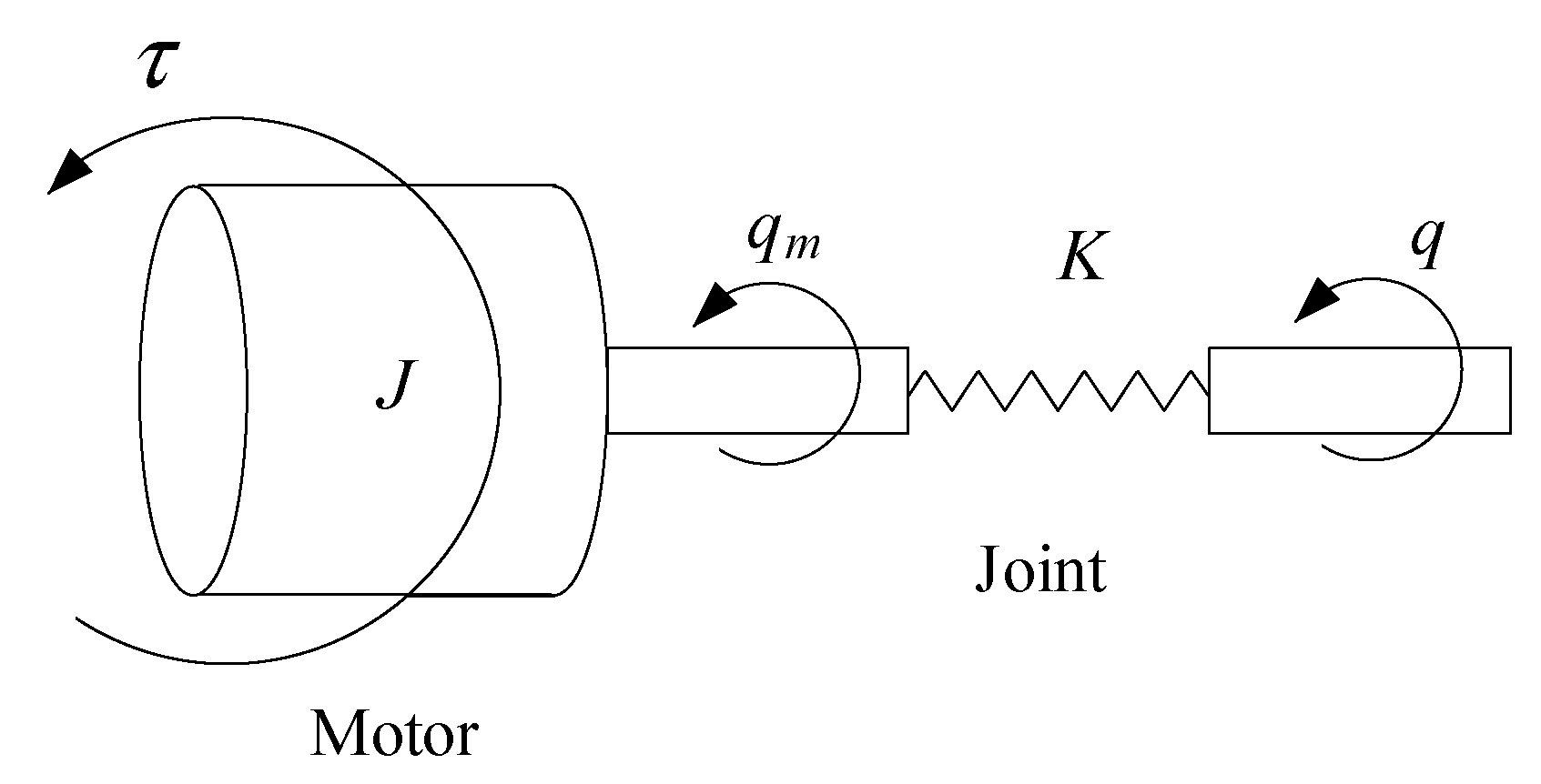
2.1. Dynamic Model of Flexible Manipulator
The flexible-joint model of a manipulator is shown in Figure 1.
The dynamic model of flexible manipulators studied in this paper is as follows.
where are the joint position, velocity and acceleration, respectively. is a symmetric positive definite inertia matrix, and is the Coriolis matrix. is the joint friction coefficient matrix. are the position, velocity and acceleration of the motor rotor angle, respectively. represents the flexibility of the model joints. represents the inertia term of the model, represents the damping term of the model joints, is the control input vector of the system. The dynamic model satisfies the following properties [24].
Property 1. is a symmetric positive definite matrix, is bounded, and , where and are normal numbers.
Property 2. is bounded, and , where is a constant and satisfies .
Let , and then system (1) is equivalently transformed into
where is the state variable of the system, and is the control input of the system. The state variable of the system satisfies the following assumption
Furthermore, we define the desired trajectory , where and are continuous and bounded.
2.2. Problem Statement
Design a nonlinear trajectory-tracking control strategy for the above state-constrained flexible manipulator system (1) to ensure that the joint position of the flexible manipulator tracks the desired trajectory . The tracking error can converge to a neighborhood near zero, that is, , when , there exists , and all state variables of the closed-loop system are continuously stable and bounded.
3. Controller Design
3.1. Error Compensation
According to the trajectory-tracking task in the problem description, the tracking error signal in the virtual control signal is defined as
where , which is output by the following command filter
where is the state of the nth command filter in ith step, and are all positive numbers, and the virtual control function is the input of the command filter.
Note that, in order to ensure that the system state converges in a finite time, the filtering error of the command filter satisfies , , , where , and are all positive numbers, , and are the convergence times of the command filter used for the first step, the second step and the third step, respectively.
In order to reduce the error existing between the virtual control signal and the finite-time command filter output signal, the error-compensation mechanism is constructed as follows
where represents the error compensation vector, and and are the tuning parameters that need to be designed.
Then, the compensated tracking error signal is designed as
Ultimately, the virtual control signals in the controller are
where and are all positive numbers, and . and are the estimated variables obtained by the adaptive update law in (21).
Remark 1.
In the process of designing the tracking controller of the flexible manipulator system using the traditional back-stepping method, each step needs to design a virtual control signal as (4) to ensure that each subsystem has the desired performance. However, using virtual controlled derivatives results in increased computational complexity. In this paper, the output of the finite-time command filter (5) is used to approximate the virtual signal and the derivative of the virtual signal to replace the calculation of the derivative of the virtual signal in the traditional back-stepping process; thereby, the computational complexity is eliminated. However, filter errors will persist until the finite-time command filter stabilizes, which will affect the control quality. Therefore, this paper proposes a finite-time error-compensation mechanism of (6) to quickly eliminate filtering errors.
3.2. Stability Analysis
This section investigates the command filtering back-stepping control strategy with state constraints and error compensation. Some necessary and sufficient conditions are derived for the main results.
If there exists a real number,and, the finite-time stable extended Lyapunov condition can be obtained by, and the convergence time .
Theorem 1.
For the flexible-joint manipulator (1), using the error-compensation mechanism in (6) and the virtual control signal in (8), the joint position track the desired joint position in a finite time, and all system states in the closed-loop system are bounded in a finite time.
Proof of Theorem 1.
The stability of the closed-loop system is proven by the following four steps.
Step 1. Select Lyapunov function , taking the time derivative of yields
Substitute and into (20) to find
Step 2. Select Lyapunov function , and taking the derivative of yields
where , .
Since the function contains uncertainty, it is approximated by a neural network [27], then can be approximately expressed as
where is the weight matrix, is the basis function vector, and is the approximation error and satisfies , .
According to the Young inequality, we can find
where is a positive number. Substitute , and into (14), we obtain
Step 3. Select Lyapunov function , and taking the derivative of yields
Substitute and into (20) to obtain
Step 4. Select Lyapunov function , and take the derivative of yields
where , . Similar to (13), can be written as
where is weight matrix, is the basis function vector, and is the approximation error and satisfies , .
In view of (18) and the Young inequality, we have
Let , , , then the estimate and of and can be obtained by the following adaptive update law
where , , , . Let , ; furthermore, we construct the following Lyapunov function , and take the derivative of , we have
where , , , . By Lemma 1, we obtain
in which
It is clear that we can find a positive number such that
Furthermore, it can be seen from Lemma 2 that, if , then we have
which indicates that will converge to the following region in finite time
The time required to reach the region in (26) is
which means that the state of the system converges in the desired neighborhood near the origin in finite time, and all control signals in the closed-loop system are bounded in finite time. □
Remark 2.In view of the definition of convergence region, it can be seen that we can obtain a smaller convergence area by increasing the parameters,.
4. Simulation
In this section, a simulation example of a single joint flexible manipulator is provided to illustrate the theoretical result. The parameter of system (1) is shown in Table 1.
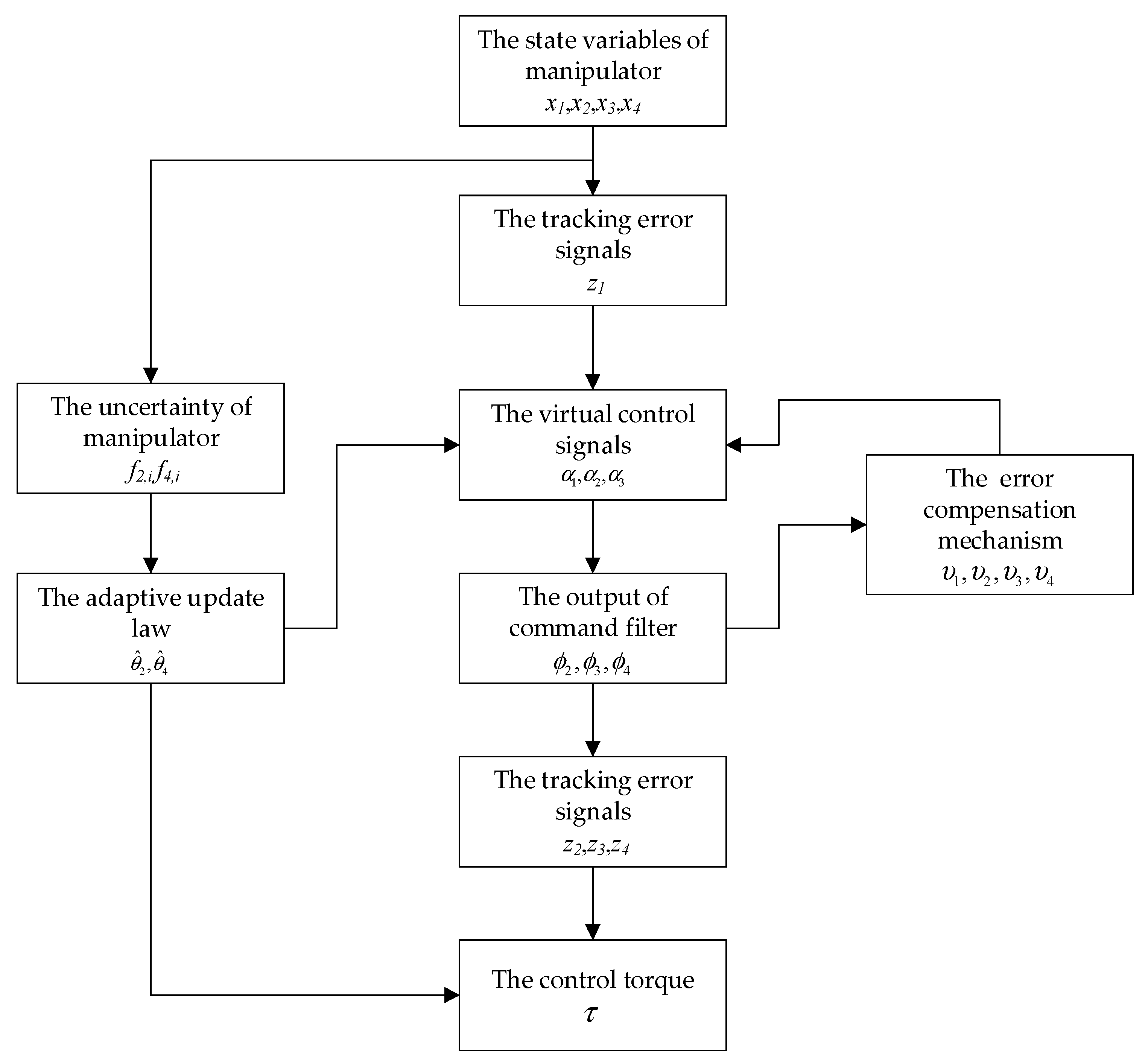
The structure diagram of the control system is shown in Figure 2.
Suppose that the desired tracking trajectory is set as , then the initial state is , . The term of joint friction is set as . The constraints of the system state are , , , , respectively.
The parameters of the command filter (5) are set as . The parameters of the error-compensation mechanism (6) are selected as , , , and . The parameters of virtual control signals (8) are set as ,, , , . The parameters of the adaptive update law (21) are set as , . The other parameters used in (22) are selected as , , .
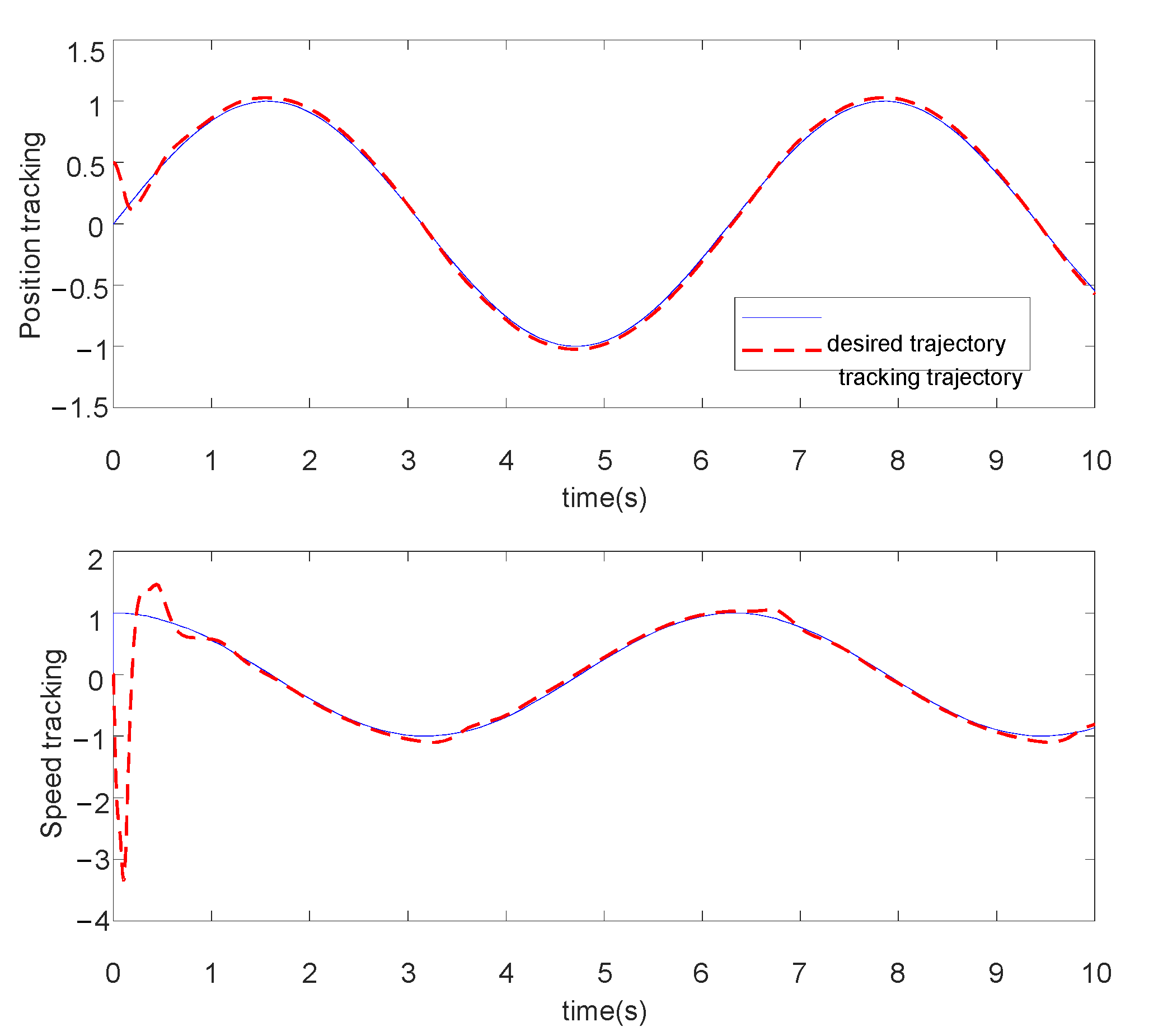
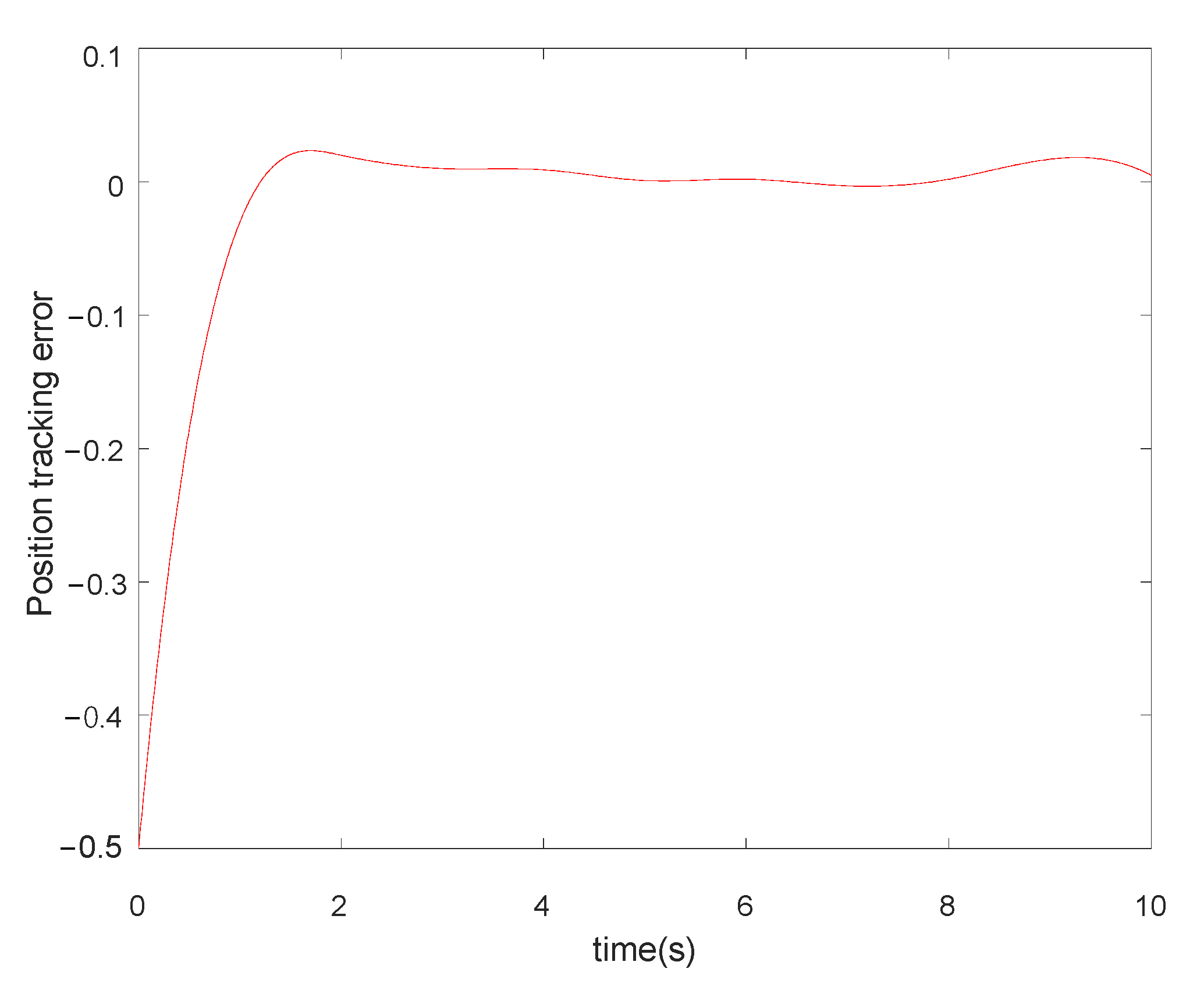
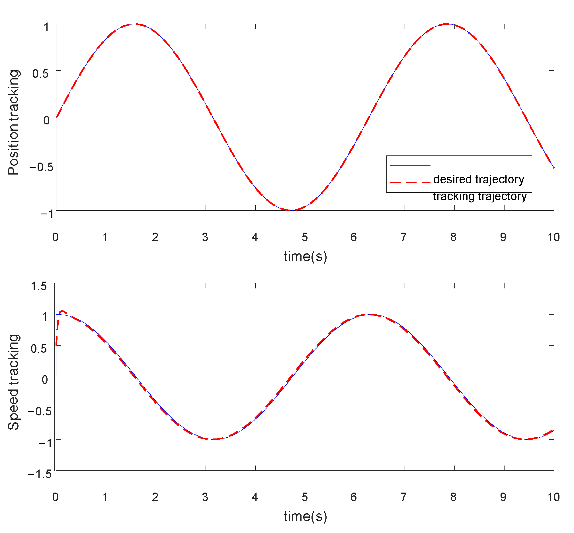
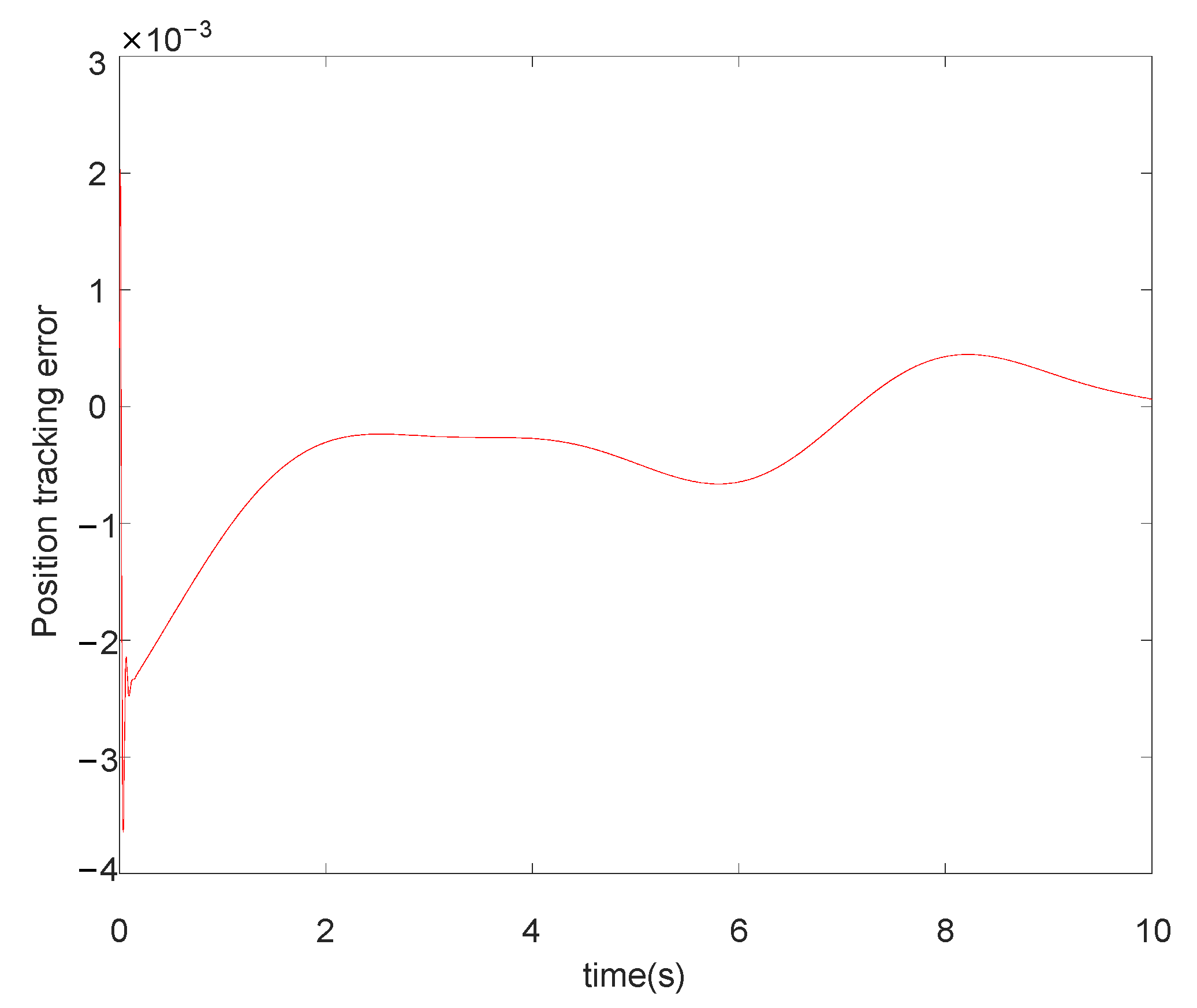
First, in order to verify the effectiveness of the error-compensation mechanism for the flexible manipulator system (1), the position and velocity tracking curves are shown in Figure 3 in the case that the error-compensation mechanism is not used in the controller, and the position tracking error curves without error compensation are shown in Figure 4. Then, the position and velocity tracking curves are shown in Figure 5 by using the error-compensation mechanism, and the position tracking error curves with error compensation are shown in Figure 6.
As can be seen from Figure 3 to Figure 6, the use of the error-compensation mechanism in the controller can improve the accuracy of the position and velocity tracking effectively. In addition, after using the error-compensation mechanism, the system state can satisfy the state constraints at the same time. Then, the effectiveness of the error-compensation mechanism designed in this paper is verified.
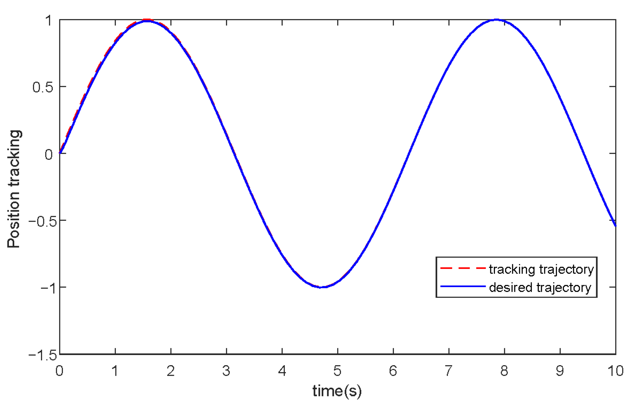
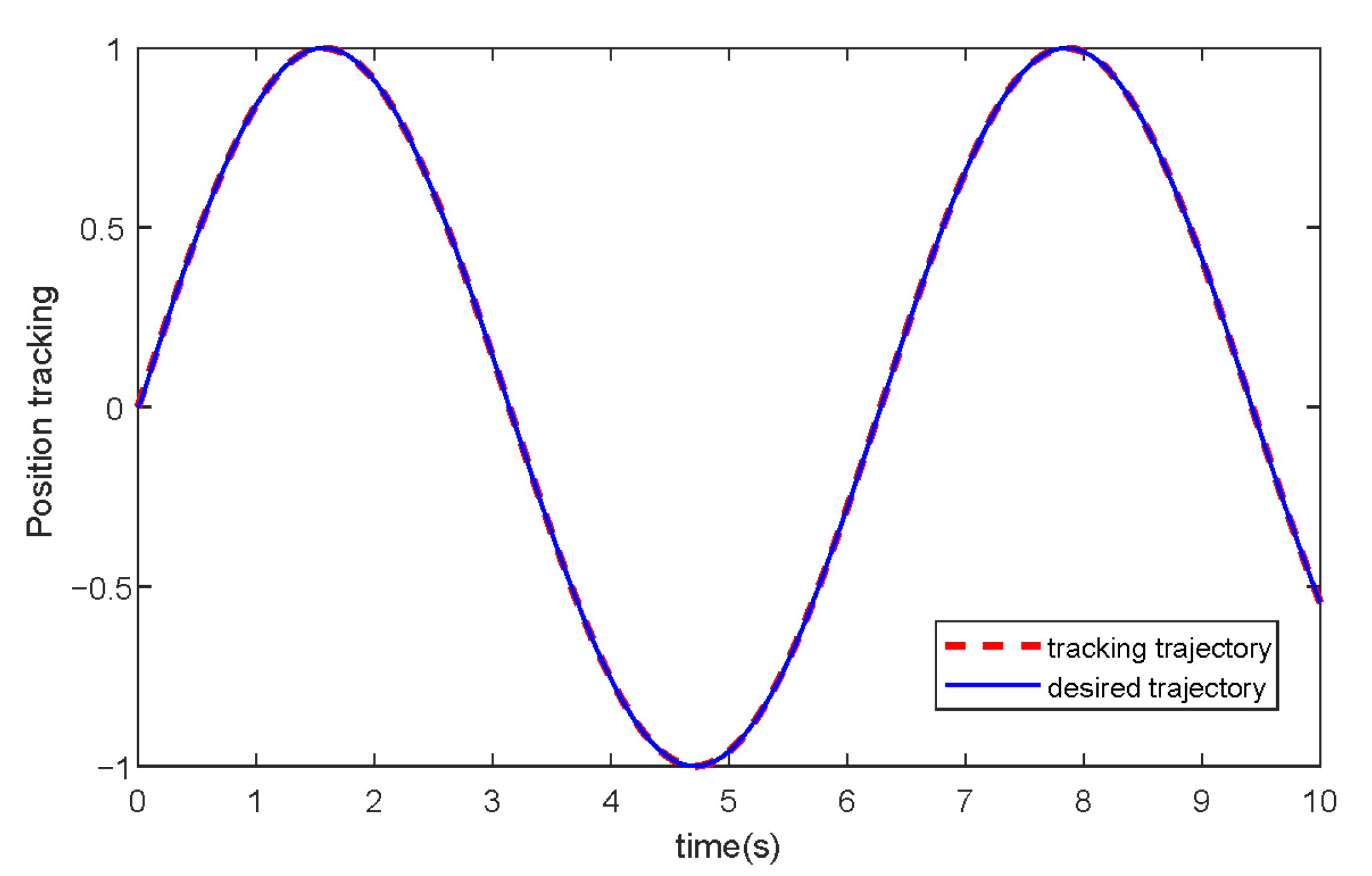
Secondly, the finite-time control effect of the control algorithm proposed in this paper is verified by adjusting parameters in the following two cases. The parameters is set as in the first case. The parameters is set as in the second case.
Figure 7 and Figure 8 show the joint position tracking curves under two different control parameters. It can be seen from Figure 7 that, in the first case, the joint trajectory can track the desired trajectory in 2.3 s, while by increasing the adjustment parameters, the joint can track the desired trajectory in 0.2 s, as shown in Figure 8. As can be seen from Figure 7 and Figure 8, we can improve the convergence efficiency by increasing the gain of the control parameters.
5. Conclusions
Aiming at the finite-time tracking-control problem of state-constrained flexible manipulator systems, this paper proposes an adaptive neural network command filtering back-stepping control method. Compared with the traditional back-stepping control, the computational complexity is eliminated by designing a finite-time command filter in the process of establishing a finite-time virtual control function, and a finite-time error-compensation mechanism is designed to eliminate errors in the filtering process. The Lyapunov function is used to verify the finite-time convergence of the closed-loop system. In future work, the method designed in this paper will be extended to a multi-joint flexible manipulator system, and an adaptive robust control method will be considered to overcome the influence of unknown external disturbances.
Author Contributions
Conceptualization, Y.Z. and M.Z.; methodology, Y.Z.; software, M.Z.; validation, Y.Z., C.F. and F.L.; formal analysis, C.F.; investigation, F.L.; resources, Y.Z.; data curation, Y.Z.; writing—original draft preparation, Y.Z.; writing—review and editing, C.F.; visualization, C.F.; supervision, Y.Z.; project administration, Y.Z.; funding acquisition, Y.Z. All authors have read and agreed to the published version of the manuscript.
Funding
This research was funded by the National Natural Science Foundation of China, grant number 61703146; the Scientific and Technological Project of Henan Province, grant number 202102110126; the Backbone teacher project of Henan Province grant number, 2020GGJS048; the key scientific research projects of colleges and universities in Henan Province, grant number 19B413002.
Institutional Review Board Statement
Not applicable.
Informed Consent Statement
Not applicable.
Data Availability Statement
Not applicable.
Conflicts of Interest
The authors declare no conflict of interest. The funders had no role in the design of the study; in the collection, analyses, or interpretation of data; in the writing of the manuscript, or in the decision to publish the results.
References
Huang, D.; Huang, X. Neural Network Compensation Control for Model Uncertainty of Flexible Space Manipulator Based on Hybrid Trajectory. J. Eng. Sci. Technol. Rev.2021, 14, 86–94. [Google Scholar]
Shin, H.C.; Choi, S.B. Position control of a two-link flexible manipulator featuring piezoelectric actuators and sensors. Mechatronics2001, 11, 707–729. [Google Scholar] [CrossRef]
Mahmood, I.A.; Moheimani, S.O.; Bhikkaji, B. Precise tip positioning of a flexible manipulator using resonant control. IEEE/ASME Trans. Mechatron.2008, 13, 180–186. [Google Scholar] [CrossRef]
Chang, W.; Li, Y.; Tong, S. Adaptive fuzzy backstepping tracking control for flexible robotic manipulator. IEEE/CAA J. Autom. Sin.2018, 8, 1923–1930. [Google Scholar] [CrossRef] [Green Version]
Sun, C.; Wei, H.; Jie, H. Neural Network Control of a Flexible Robotic Manipulator Using the Lumped Spring-Mass Model. IEEE Trans. Syst. Man Cybern. Syst.2017, 47, 1863–1874. [Google Scholar] [CrossRef]
Reddy, M.; Jacob, J. Vibration Control of Flexible Link Manipulator Using SDRE Controller and Kalman Filtering. Stud. Inform. Control.2017, 26, 143–150. [Google Scholar]
Belherazem, A.; Chenafa, M. Passivity Based Adaptive Control of a Single-Link Flexible Manipulator. Autom. Control Comput. Sci.2021, 55, 1–14. [Google Scholar] [CrossRef]
Cao, F.; Liu, J. An adaptive iterative learning algorithm for boundary control of a coupled ODE–PDE two-link rigid–flexible manipulator. J. Frankl. Inst.2016, 354, 277–297. [Google Scholar] [CrossRef]
Yao, W.; Guo, Y.; Wu, Y.F. Robust Adaptive Dynamic Surface Control of Multi-link Flexible Joint Manipulator with Input Saturation. Int. J. Control Autom. Syst.2022, 20, 577–588. [Google Scholar] [CrossRef]
Kivila, A.; Book, W.; Singhose, W. Modeling spatial multi-link flexible manipulator arms based on system modes. Int. J. Intell. Robot. Appl.2021, 5, 300–312. [Google Scholar] [CrossRef]
Ji, N.; Liu, J. Vibration control for a flexible satellite with input constraint based on Nussbaum function via backstepping method. Aerosp. Sci. Technol.2018, 77, 563–572. [Google Scholar] [CrossRef]
Cao, F.; Liu, J. Three-dimensional modeling and input saturation control for a two-link flexible manipulator based on infinite dimensional model. J. Frankl. Inst.2020, 357, 1026–1042. [Google Scholar] [CrossRef]
Zhang, S.J.; Cao, Y. Cooperative Localization Approach for Multi-Robot Systems Based on State Estimation Error Compensation. Sensors2019, 19, 3842. [Google Scholar] [CrossRef] [PubMed] [Green Version]
Zhu, X.; Shen, X.; Wang, L. Tip Tracking Control of a Linear-Motor-Driven Flexible Manipulator with Controllable Damping. IFAC-Pap.2020, 53, 9163–9168. [Google Scholar] [CrossRef]
Xing, X.; Liu, J. PDE model-based state-feedback control of constrained moving vehicle-mounted flexible manipulator with prescribed performance. J. Sound Vib.2019, 441, 126–151. [Google Scholar] [CrossRef]
Ma, X.; Wang, P.; Ye, M. Shared Autonomy of a Flexible Manipulator in Constrained Endoluminal Surgical Tasks. IEEE Robot. Autom. Lett.2019, 4, 3106–3112. [Google Scholar] [CrossRef]
Cheng, X.; Liu, H.S. Bounded decoupling control for flexible-joint robot manipulators with state estimation. IET Control Theory Appl.2020, 14, 2348–2358. [Google Scholar] [CrossRef]
Zhang, S.; Cao, Y. Consensus in networked multi-robot systems via local state feedback robust control. Int. J. Adv. Robot. Syst.2019, 16, 1729881419893549. [Google Scholar] [CrossRef]
Tang, Y.; Xing, X.; Karimi, H.R. Tracking control of networked multi-agent systems under new characterizations of impulses and its applications in robotic systems. IEEE Trans. Ind. Electron.2016, 63, 1299–1307. [Google Scholar] [CrossRef]
Xia, Y.; Zhang, J.; Lu, K.; Zhou, N. Finite-Time Tracking Control of Rigid Spacecraft Under Actuator Saturations and Faults. IEEE Trans. Autom. Sci. Eng.2016, 18, 368–381. [Google Scholar]
Anjum, Z.; Guo, Y.; Yao, W. Fault tolerant control for robotic manipulator using fractional-order backstepping fast terminal sliding mode control. Trans. Inst. Meas. Control2021, 43, 3244–3254. [Google Scholar] [CrossRef]
Zhao, Z.; Liu, Z. Finite-Time Convergence Disturbance Rejection Control for a Flexible Timoshenko Manipulator. IEEE/CAA J. Autom. Sin.2021, 8, 161–172. [Google Scholar] [CrossRef]
Qiu, J.; Sun, K.; Rudas, I.J.; Gao, H. Command Filter-Based Adaptive NN Control for MIMO Nonlinear Systems with Full-State Constraints and Actuator Hysteresis. IEEE Trans. Cybern.2020, 50, 2905–2915. [Google Scholar] [CrossRef] [PubMed]
Huang, A.C.; Chen, Y.C. Adaptive sliding control for single-link flexible-joint robot with mismatched uncertainties. IEEE Trans. Control Syst. Technol.2004, 12, 770–775. [Google Scholar] [CrossRef]
Abdollahi, F.; Talebi, H.A.; Patel, R.V. A stable neural network based observer with application to flexible-joint manipulators. IEEE Trans. Neural Netw.2006, 17, 118–129. [Google Scholar] [CrossRef]
Yu, S.H.; Yu, X.H.; Shirinzadeh, B. Continuous finite-time control for robotic manipulators with terminal sliding mode. Automatica2005, 41, 1957–1964. [Google Scholar] [CrossRef]
Wang, D.H.; Zhang, S.J. Improved neural network-based adaptive tracking control for manipulators with uncertain dynamics. Int. J. Adv. Robot. Syst.2020, 17, 1823–1838. [Google Scholar] [CrossRef]
Figure 1.
The flexible-joint model of a manipulator.
Figure 1.
The flexible-joint model of a manipulator.
Figure 2.
The structure diagram of the control system.
Figure 2.
The structure diagram of the control system.
Figure 3.
Position and velocity tracking curves without error compensation.
Figure 3.
Position and velocity tracking curves without error compensation.
Figure 4.
Position tracking error curves without error compensation.
Figure 4.
Position tracking error curves without error compensation.
Figure 5.
Position and velocity tracking curves with error compensation.
Figure 5.
Position and velocity tracking curves with error compensation.
Figure 6.
Position tracking error curves with error compensation.
Figure 6.
Position tracking error curves with error compensation.
Figure 7.
Position tracking curves under the first case.
Figure 7.
Position tracking curves under the first case.
Figure 8.
Position tracking curves under the second case.
Figure 8.
Position tracking curves under the second case.
Table 1.
Parameters of the flexible manipulator.
Table 1.
Parameters of the flexible manipulator.
Parameters
Value
M
0.2/kg
L
0.3/m
g
9.8/m/s2
K
6.47/N·m/rad
B
0.01
J
0.21/ m/s2
Publisher’s Note: MDPI stays neutral with regard to jurisdictional claims in published maps and institutional affiliations.
Zhang, Y.; Zhang, M.; Fan, C.; Li, F.
A Finite-Time Trajectory-Tracking Method for State-Constrained Flexible Manipulators Based on Improved Back-Stepping Control. Actuators2022, 11, 139.
https://0-doi-org.brum.beds.ac.uk/10.3390/act11050139
AMA Style
Zhang Y, Zhang M, Fan C, Li F.
A Finite-Time Trajectory-Tracking Method for State-Constrained Flexible Manipulators Based on Improved Back-Stepping Control. Actuators. 2022; 11(5):139.
https://0-doi-org.brum.beds.ac.uk/10.3390/act11050139
Chicago/Turabian Style
Zhang, Yiwei, Min Zhang, Caixia Fan, and Fuqiang Li.
2022. "A Finite-Time Trajectory-Tracking Method for State-Constrained Flexible Manipulators Based on Improved Back-Stepping Control" Actuators 11, no. 5: 139.
https://0-doi-org.brum.beds.ac.uk/10.3390/act11050139
Note that from the first issue of 2016, this journal uses article numbers instead of page numbers. See further details here.
Article Metrics
No
No
Article Access Statistics
For more information on the journal statistics, click here.
Multiple requests from the same IP address are counted as one view.
Zhang, Y.; Zhang, M.; Fan, C.; Li, F.
A Finite-Time Trajectory-Tracking Method for State-Constrained Flexible Manipulators Based on Improved Back-Stepping Control. Actuators2022, 11, 139.
https://0-doi-org.brum.beds.ac.uk/10.3390/act11050139
AMA Style
Zhang Y, Zhang M, Fan C, Li F.
A Finite-Time Trajectory-Tracking Method for State-Constrained Flexible Manipulators Based on Improved Back-Stepping Control. Actuators. 2022; 11(5):139.
https://0-doi-org.brum.beds.ac.uk/10.3390/act11050139
Chicago/Turabian Style
Zhang, Yiwei, Min Zhang, Caixia Fan, and Fuqiang Li.
2022. "A Finite-Time Trajectory-Tracking Method for State-Constrained Flexible Manipulators Based on Improved Back-Stepping Control" Actuators 11, no. 5: 139.
https://0-doi-org.brum.beds.ac.uk/10.3390/act11050139
Note that from the first issue of 2016, this journal uses article numbers instead of page numbers. See further details here.


