
Research on PID Position Control of a Hydraulic Servo System Based on Kalman Genetic Optimization


College of Mechanical and Electronic Engineering, Nanjing Forestry University, Nanjing 210037, China
*
Author to whom correspondence should be addressed.
Actuators 2022, 11(6), 162; https://0-doi-org.brum.beds.ac.uk/10.3390/act11060162
Submission received: 12 May 2022
/
Revised: 8 June 2022
/
Accepted: 13 June 2022
/
Published: 15 June 2022
(This article belongs to the Special Issue Vibration Control and Structure Health Monitoring)
Abstract
:With the wide application of hydraulic servo technology in control systems, the requirement of hydraulic servo position control performance is greater and greater. In order to solve the problems of slow response, poor precision, and weak anti-interference ability in hydraulic servo position controls, a Kalman genetic optimization PID controller is designed. Firstly, aiming at the nonlinear problems such as internal leakage and oil compressibility in the hydraulic servo system, the mathematical model of the hydraulic servo system is established. By analyzing the working characteristics of the servo valve and hydraulic cylinder in the hydraulic servo system, the parameters in the mathematical model are determined. Secondly, a genetic algorithm is used to search the optimal proportional integral differential (PID) controller gain of the hydraulic servo system to realize the accurate control of valve-controlled hydraulic cylinder displacement in the hydraulic servo system. Under the positioning benchmark of step signal and sine wave signal, the PID algorithm and the genetic optimized PID algorithm are compared in the system simulation model established by Simulink. Finally, to solve the amplitude fluctuations caused by the GA optimized PID and reduce the influence of external disturbances, a Kalman filtering algorithm is added to the hydraulic servo system to reduce the amplitude fluctuations and the influence of external disturbances on the system. The simulation results show that the designed Kalman genetic optimization PID controller can be better applied to the position control of the hydraulic servo system. Compared with the traditional PID control algorithm, the PID algorithm optimized by genetic algorithm improves the system’s response speed and control accuracy; the Kalman filter is a good solution for the amplitude fluctuations caused by GA-optimized PID that reduces the influence of external disturbances on the hydraulic servo system.
1. Introduction
Hydraulic systems are widely used in industrial and mobile applications due to their high power to mass ratio and reliability. As a closed-loop control hydraulic system, the hydraulic servo system has the advantages of a hydraulic system and has the characteristics of fast response and high servo accuracy. Therefore, a hydraulic servo system is widely used in automation direction. In recent years, research on hydraulic servo systems has focused on trajectory tracking, state estimation, fault diagnosis, and parameter identification to achieve high-performance control [1]. One of the most desirable requirements is high precision position control with fast response, especially for valve-operated hydraulic cylinders, the actuators of hydraulic servo systems.
The accurate modeling of the controlled object is essential for the position control of the hydraulic servo system. Establishing an accurate mathematical model of the hydraulic servo system is very complicated due to the dead zone in the flow region, the static friction of the fluid, the compressibility and internal leakage of the fluid, the complex flow pressure characteristics of the control valve, and other factors that lead to the problem of a highly nonlinear and largely uncertain hydraulic servo system. In the last few years, some important work has been carried out by related researchers in the modeling of hydraulic servo systems. Xing et al. [2] analyzed the functions of servo valves and hydraulic cylinders and established the transfer function of an automatic depth-controlled electrohydraulic system using a first-principles approach. Mete et al. [3] considered the effects of compressibility, friction, servo valve internal leakage, actuator leakage, and inertia on the electro-hydraulic servo system and established a mathematical model of the main components of the internal leakage electro-hydraulic servo system. Zheng et al. [4] considered the problems of dead zones, saturation nonlinearity, time lag, and time variability in servo-hydraulic presses. Yao et al. [5] used the known information of the electro-hydraulic servo system to build an adaptive inverse model of the system. For the system’s nonlinear parameters, online estimation was used to adapt the dynamic inverse model in real-time. Ye et al. [1] considered nonlinear factors such as dead zone, saturation, discharge coefficient, and friction during modeling a valve-controlled cylinder system for a hydraulic excavator. Li et al. [6] constructed adaptive parts of the hydraulic actuator model with parameter uncertainty to handle it, and considered the residuals of parameter adaptation and the unmodeled dynamics part with a robust part. Shen et al. [7] analyzed the basic principles of the new hydraulic transformer, established a mathematical model of the system, and simplified the state-space equations of the system by making appropriate assumptions about the system. Knohl and Unbehauen [8] studied the problem of large dead zones of valves in electro-hydraulic servo systems by linearizing the cylinder and load forces as a second-order system and integrator while connecting the dead zone part and the linear part in a series to describe the hydraulic system. Bao et al. [9] implemented a multi-pump, multi-actuator hydraulic system modeling based on the dynamic analysis of hydraulic systems. Zhang et al. [10] trained a BP neural network model to obtain a nonlinear relationship between motor speed and cylinder two-chamber pressure as input and cylinder speed as output and constructed a soft measurement model for the position of the direct-drive hydraulic system by integrating the calculated speed of the network. Nguyen et al. [11] investigated the motion dynamics of actuators under torque in a mechanical system considering parameter uncertainties, unmodeled uncertainties, and perturbations. They realized the position model of the electro-hydraulic servo system with detailed analysis of servo valve and hydraulic system models. Zhang et al. [12] considered the clearance problem between spool and sleeve in the construction of the mathematical model of the nonlinear position servo control system of magnetically coupled rodless hydraulic cylinders, established the mass flow relationship of each valve port by analyzing the proportional control valve structure and through experimental tests, and used the friction model after experimental tests for the friction model of the valve-controlled cylinder, so as to realize the establishment of the system dynamics equations. These studies provide some methods for solving nonlinear problems in modeling hydraulic servo systems.
In addition, to achieve good position control, it is necessary to study the control methods used in the hydraulic servo system, such as PID, fuzzy algorithm, neural network optimization, etc. PID control has been commonly used in hydraulic systems with the advantages of simple structure, easy implementation, and mature theoretical analysis. The critical step in PID control is the effective adjustment of three adjustable gains: proportional gain, integral gain, and differential gain. However, PID control has linear characteristics and cannot meet the requirements of nonlinear systems alone. In recent decades, many intelligent optimization techniques have been used to regulate PID gains to solve the control problems of nonlinear and complex systems. Chang [13] used an artificial bee colony (ABC) algorithm to search for PID control parameters to enhance the control performance of a continuously stirred kettle reactor. He [14] proposed an improved artificial bee colony algorithm to optimize the gain of the PID controller and improve the control performance of the strip deviation control system. Hao et al. [15] used the particle swarm optimization (PSO) algorithm to optimize the PID parameters and improved PSO in inertia weights, learning coefficients, and elite variances to improve trajectory tracking accuracy in electro-hydraulic position servo systems. Zheng et al. [4] introduced a fuzzy PID control method to improve the overall performance of the electro-hydraulic position servo system to establish fuzzy inference rules capable of adaptively adjusting the PID parameters in terms of the error and error variation of the system. Wang et al. [16] introduced a fuzzy controller based on the particle swarm algorithm to rectify the parameters of the PID. Shutnan et al. [17] used the clone selection algorithm to rectify the PID parameters for the path tracking problem of a robotic manipulator. Guo et al. [18] combined PID control and generalized predictive control to exploit the advantages of each and improve the system performance. Odili et al. [19] applied the African Buffalo Optimization algorithm to rectify the PID controller parameters for effective control of the voltage regulator (AVR). Bingul et al. [20] used the cuckoo search algorithm to optimize the design of the PID controller parameters in an AVR system. Loucif [21] used a novel optimization algorithm of the Whale Optimization Algorithm to determine the optimal parameters of the PID controller to achieve better trajectory tracking of the robot operator. Xue et al. [22] proposed an advanced flaring (AFW) algorithm based on the adaptive principle and bimodal Gaussian function and established a PID parameter rectification model combined with AFW. Gao et al. [23] proposed an artificial fish swarm algorithm, which has a good optimization effect on the PID of the motion servo control system. Liu et al. [24] proposed a method for intelligent tuning of PID parameters based on iterative learning control, enabling the PID parameters of the AFM to be self-tuned according to the shape of the sample. Li [25] proposed a PID control strategy based on bacterial foraging optimization to improve the performance of variable air volume-air conditioning systems. Liu et al. [26] proposed an improved fruit fly optimization algorithm that combines a PID control strategy with a cloud model algorithm to improve the response performance of a magnetorheological liquid brake proportional-integral differential controller.
Genetic algorithms (GA) are inspired by natural selection and have stochastic optimization properties to optimize any problem without prior knowledge. It also provides faster convergence to near-optimal solutions [27]. At the same time, compared to traditional optimization algorithms that obtain optimal solutions by a single initial value iteration, genetic algorithms can evolve by searching for multiple solutions in the space simultaneously, thus reducing the risk of falling into a local optimum [28,29,30]. Therefore, the study of the adaptive adjustment of PID parameters using a genetic algorithm has certain reliability and development.
This paper implements modeling of the system by considering nonlinear factors such as internal leakage and oil compressibility of the system. To address the problems of slow response and low accuracy in the position control of valve-controlled hydraulic servo systems, the PID control is used as the basis to improve the performance of the system. In this work, a GA algorithm is used to search the PID parameters to improve the control performance of the system. To solve the amplitude fluctuations caused by the GA algorithm-optimized PID controller in the position response of the hydraulic servo system and to reduce the influence of external disturbances on the system, a Kalman filter is added to the designed GA-optimized PID controller to improve the anti-interference capability of the system.
2. Valve-Controlled Hydraulic Servo System Model
2.1. Valved Hydraulic Servo System
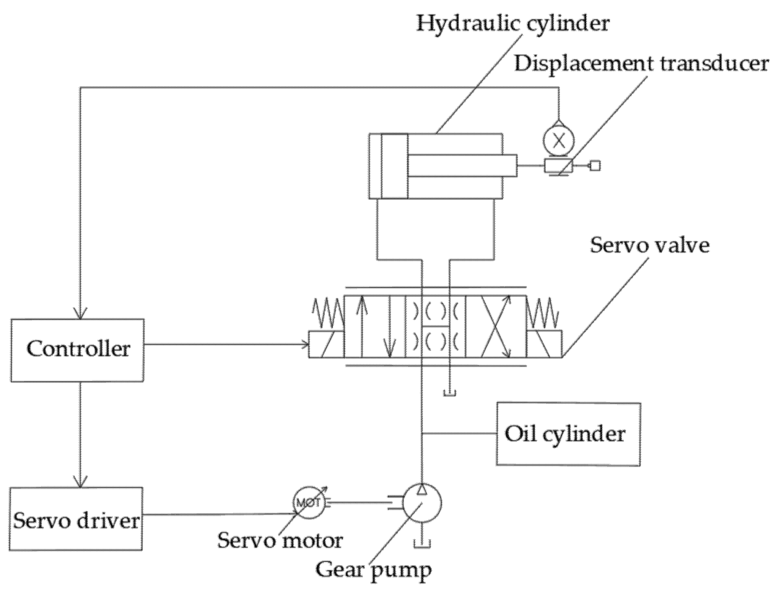
As shown in Figure 1, the valve-controlled hydraulic servo system has the following operating principles. The system consists of eight parts: hydraulic cylinder, displacement sensor, servo valve, gear pump, oil cylinder, servo motor, servo driver, and controller. The servo driver starts the servo motor and controls the speed of the motor as well as forward and reverse rotation. The servo driver starts the servo motor and controls the speed of the motor and forward and reverse rotation, and the servo motor drives the gear pump to rotate. When the servo motor is turning, the gear pump is turning, the cylinder side is the suction chamber, the gear teeth in the suction chamber are disengaged one after another, the suction tube sucks in oil from the cylinder under atmospheric pressure, and the system side is the pressure chamber, the pressure chamber is engaged one after another, and the oil sucked in by the suction tube is squeezed. The oil is delivered to the system side. When the servo motor reverses, the gear pump reverses. The cylinder side is the pressure chamber, the system side is the suction chamber, and the oil is delivered to the cylinder from the system side. The controller controls the opening of the servo valve through the voltage amount. The opening of the servo valve determines the amount of oil in and out of the hydraulic cylinder. The servo valve opening is large, and the oil entering the hydraulic cylinder from the system side of the oil output from the hydraulic cylinder to the system side is more. Thus, the displacement of the hydraulic cylinder movement is large, and vice versa, the displacement is small. The displacement of the movement is fed back to the controller through the displacement sensor at the top of the hydraulic cylinder, forming a closed-loop control loop.
2.2. Mathematical Modeling of Valve-Controlled Hydraulic Servo System
2.2.1. Hydraulic Cylinder Modeling
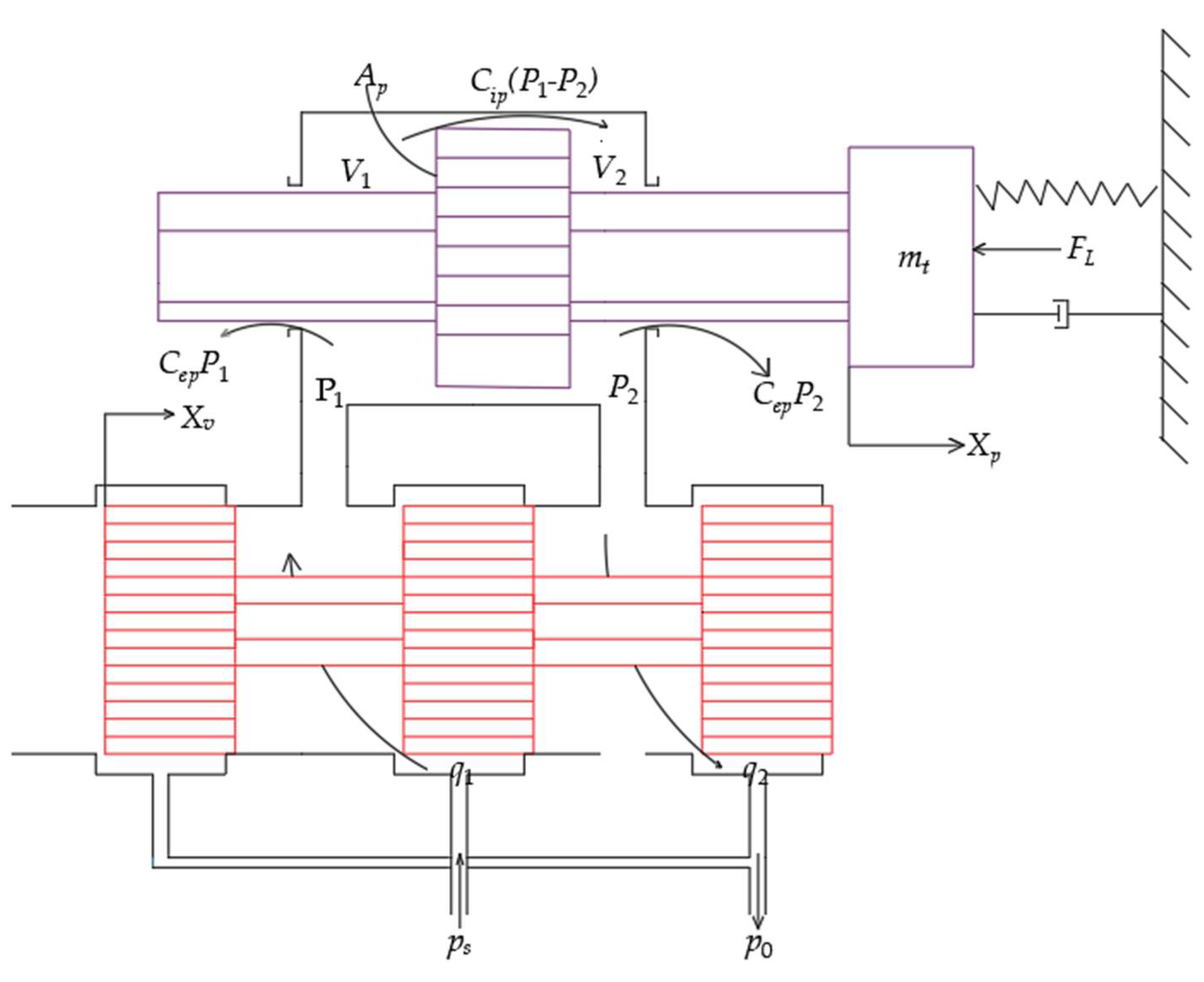
The principle of the valve-controlled hydraulic cylinder is shown in Figure 2. Among them, is the system oil supply pressure; is the return pressure of the system; is the inflow flow rate of the hydraulic cylinder inlet chamber; is the outflow flow rate of the hydraulic cylinder return chamber; and is the input displacement of the slide valve spool. and are the pressure of the oil inlet chamber and the oil return chamber, respectively; is the external leakage coefficient of the hydraulic cylinder; and are the external leakage flow at the sealed piston rod; is the internal leakage coefficient of the hydraulic cylinder; and is the internal leakage flow at the sealed piston rod, where is the load pressure, equivalent to . and are the volume of the oil inlet chamber and the oil return chamber, respectively. is the effective area of the hydraulic cylinder piston; is the sum of the converted mass of the piston end load and the piston mass; is the force of any accidental load force on the piston; and is the displacement of the hydraulic cylinder piston.
A slide valve is studied with four symmetrical throttling windows, with constant supply pressure and zero return pressure [31]. The linearized flow equation of the valve is as follows.
where is the system load flow rate; is the flow gain of the slide valve; and is the flow pressure coefficient of the slide valve. Due to leaks and the effect of fluid compressibility, the flow into and out of the hydraulic cylinder is unequal. To simplify the analysis process, is defined as
According to the inflow flow rate , outflow flow rate can be obtained [32].
where is the total leakage coefficient of the hydraulic cylinder; ; is the total compression volume of the working chamber of the hydraulic cylinder; and ; is the effective volume modulus of elasticity. The load characteristics will impact the dynamic characteristics of the hydraulic power element, and the load force generally contains damping force, inertia force, elastic force, etc. The equilibrium equation between the output force of the hydraulic cylinder and the load force is shown in Equation (4) [31].
where is the viscous damping factor corresponding to the piston and the load and is the stiffness corresponding to the load spring. Equations (1), (3), and (4) describe the dynamic characteristics of the valve-controlled hydraulic cylinder. In order to facilitate the analysis of the system characteristics, the form of the transfer function is used instead of a differential Equation to describe the dynamic characteristics of the valve-controlled hydraulic cylinder. The Laplace transformation of Equations (1), (3), and (4) yields Equation (5).
Since the input of the system is , , and the output is , to obtain the relationship between the input and output, the intermediate variables , in Equation (5) are eliminated to obtain Equation (6).
where is the total flow pressure coefficient, and . In the hydraulic servo system, generally, ; therefore, Equation (6) can be simplified as follows.
When the load stiffness is 0.
Then, when under external no-load, equals to 0, the transfer function between the displacement of the piston of the hydraulic cylinder and the input displacement of the spool is
Let
where is the spring stiffness of the hydraulic pressure; is the hydraulic inherent frequency; and is the damping ratio of the hydraulic pressure.
According to Equations (10)–(12), Equation (9) can be expressed as
The no-load flow characteristic is the characteristic flow corresponding to the load pressure drop , which is known from (1).
Equation (15) is obtained from Equations (13) and (14).
2.2.2. Servo Valve Modeling
The input signal of the electro-hydraulic servo valve is the current signal. The output signal is the no-load flow signal of the servo valve. Its essence is a nonlinear element. The form of its transfer function used depends on the magnitude of the hydraulic intrinsic frequency of the power element. When the servo valve bandwidth is close to the hydraulic intrinsic frequency, the servo valve can be approximated as a second-order oscillatory system.
where is the flow gain of the servo valve; is the intrinsic frequency of the servo valve; and is the damping ratio of the servo valve.
2.2.3. Mathematical Modeling of the Valve-Controlled Hydraulic Servo System
According to the parameters of the hydraulic cylinder and the servo valve, see Table 1, the specific servo valve and the hydraulic cylinder model can be determined.
The displacement command signal input by the system is a voltage signal, and the input signal of the servo valve is a current signal, so it is necessary to add a servo amplifier between the system input and the servo valve. After comparing and amplifying the input displacement command signal (voltage signal) and the displacement feedback signal (voltage signal) of the system, a control current proportional to the deviation voltage is output to the servo valve. The amplification factor of the servo amplifier is:
where is the deviation between the input displacement signal and the feedback displacement signal . The displacement command signal input by the system takes a voltage signal of as the input, and the input current of the electro-hydraulic servo valve is . It can be determined that is equal to 0.004.
The output signal of the valve-controlled hydraulic servo system is a displacement signal, and the feedback signal is a displacement signal. In order to compare it with the input signal, a feedback amplifier is added to convert the displacement signal into a voltage signal. The amplification factor of the feedback amplifier is:
The movable working stroke of the hydraulic cylinder is , and the input voltage of the system is , from which can be determined to be equal to 90.9.
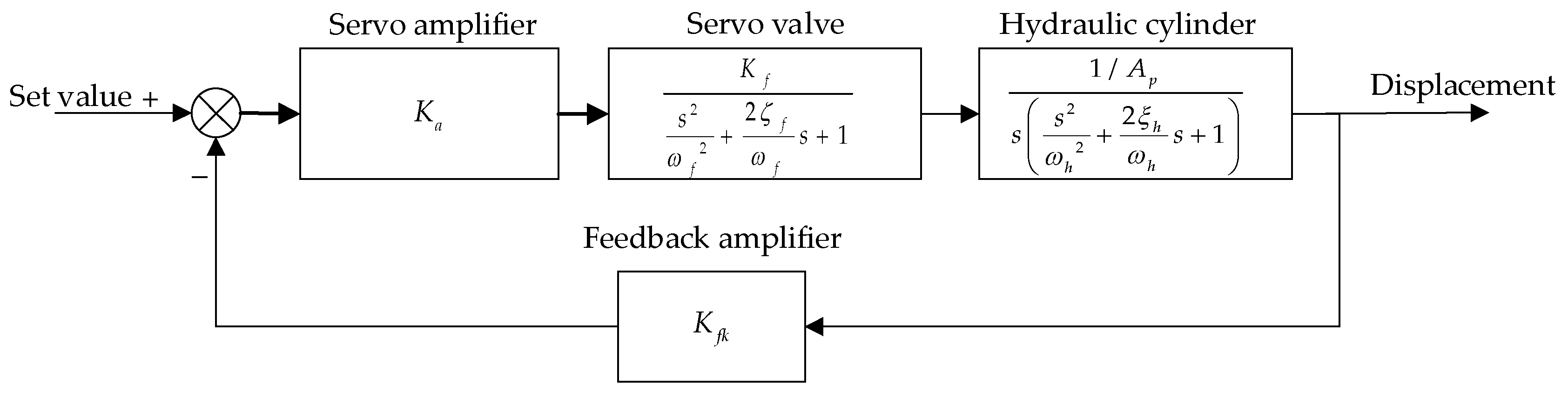
According to the mathematical model of each part of the hydraulic servo system, the control flow chart of the hydraulic servo valve control system is established as shown in Figure 3.
3. Control Algorithm of Hydraulic Servo System
3.1. PID Control Algorithm
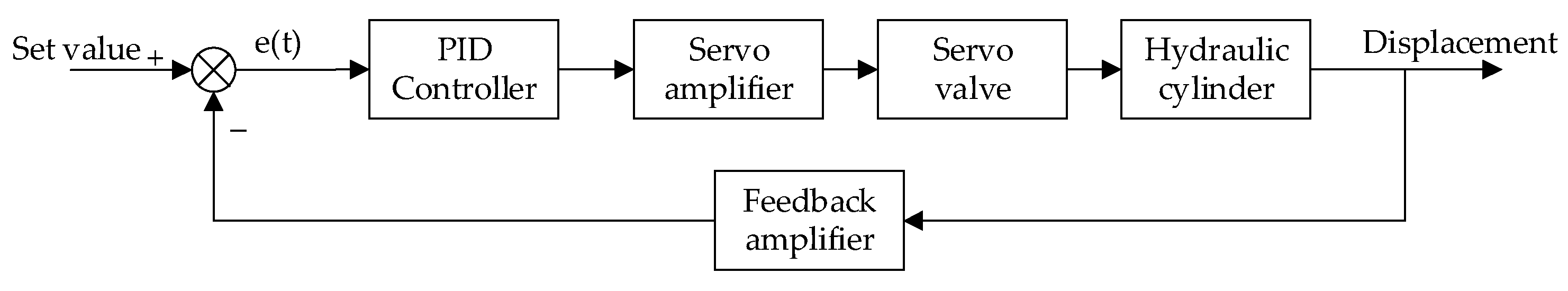
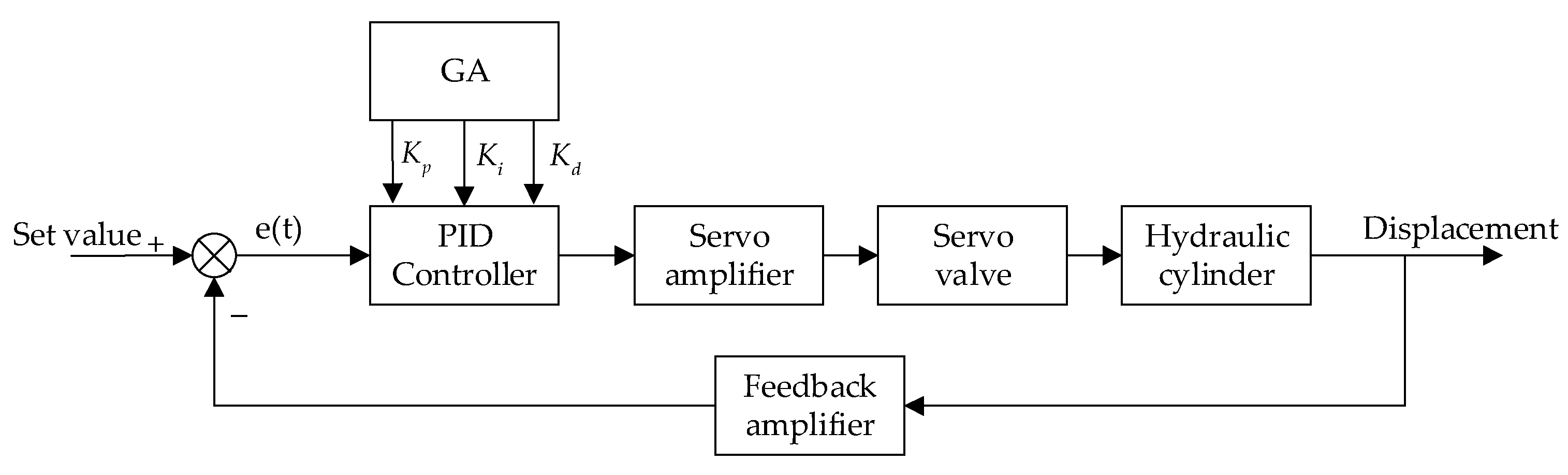
In the closed-loop control system, the PID controller is widely used in the industry. It has the advantages of good stability, convenient adjustment, and high reliability [6,7]. Using the PID controller for position control in the hydraulic servo system, as shown in Figure 4, can increase the accuracy and response speed of the hydraulic servo position control to some extent.
PID control consists of three units: proportional, integral, and differential. PID control adapts to different system requirements by adjusting the gain value of these three units. The PID controller can be expressed as the following mathematical formula [33]:
where is defined as the output function of the controller at time ; is the proportional coefficient; is the integral coefficient; is the differential coefficient; is the error ( equals the set value minus the feedback value); is the current time; and is the integral variable. Its expression in the continuous domain is:
The performance of the PID controller depends on the appropriateness of the selection of the PID gain parameter. Although the gain of the three units of the PID is easy to adjust, different system transfer functions correspond to different PID gain parameters. In the process of gain adjustment, the three units will conflict, resulting in the PID controller not achieving a better performance. Therefore, the gain parameters corresponding to the three units of the PID need to be traded off to obtain the best overall control results. So the key to the PID controller is to adjust the adjustable parameters.
3.2. Optimization of the PID Algorithm by Genetic Algorithm
At present, many optimization methods are used to adjust the PID controller parameters, such as PSO, ABC, and so on. ABC can avoid falling into local optimal stagnation in optimization, but it will have the problem of slow convergence; the PSO algorithm converges fast, but easily falls into the local optimal solution and is unstable [34]. Compared with the above intelligent algorithms, the GA can obtain the global optimal solution according to the principle of natural evolution and converge quickly. The PID controller optimized by GA is used in the hydraulic servo system, as shown in Figure 5, so that the output response can better track the target.
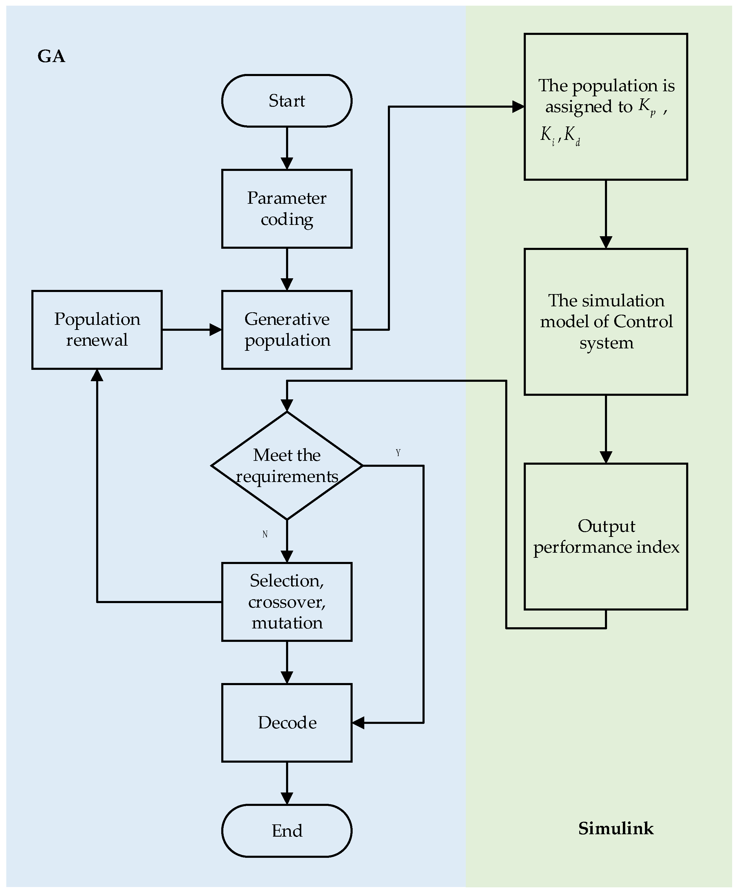
GA represents an evolutionary process similar to the Darwinian model. This process begins with the creation of an initial random group of individuals. These individuals, the points in the state space, adopt the value of the criterion to be optimized. It goes through the stages of selection, hybridization, and mutation from one generation to another to produce a new population for the next generation. The evaluation of the fitness function makes it possible to provide the optimal solution of the generation under consideration until the unique optimal solution is imposed by the convergence condition of the iterative system [35]. In order to overcome the shortcomings of the PID algorithm, the GA with crossover and mutation operation is used to adjust and optimize the three parameters of PID. GA can flexibly construct a heuristic process and corresponding objective function and can randomly and quickly search the optimal solution and find the global optimal solution in the process of a parameter search. The specific process is as follows:
- Code and population initialization:
Coding is the process of converting the three parameters, , , and , in the PID into chromosomes that genetic algorithms can manipulate. The content of the coding is to correspond the genotypes of individuals in biology to potentially feasible solutions. In this paper, the real number coding method is adopted, and the integer in the given range 0 to 9 is used to represent the parameters. The Ziegler-Nichols method is used to determine the optimization interval of PID parameters. The sequence of N, randomly generated [,,], is used as the initial cluster, while the maximum evolutionary generation is set considering the complexity of the calculation.
- 2.
- Calculate the value of individual fitness function:
The absolute value time-integrated performance index of the system error is used as the minimum objective function value of the parameter, and the optimal index for parameter selection is
Among them, is the optimal index, is the absolute value of error, and is the system adjustment time. A penalty factor is added to the optimal index . In order to avoid the appearance of overshoot and prevent the response time from being slow due to the long rise time, the amount of overshoot is taken as one of the optimal indexes when overshoot occurs, and the rise time is taken as one of the optimal indexes when the response is slow, at which time the optimal index is
Among them, is the system overshoot, is the rise time of the system and , , , and are the weights corresponding to , , and . The choice of weights affects the corresponding performance. Adjusting the relative sizes of , , , and can indicate the importance given to , , , and . In the program simulation for test debugging, is set to 0.5, the value of is set to 0.4, is set to 0.9, and is set to 0.4. The fitness function is a tool to determine the genotypic performance of an individual. It can be seen as the driving force for individuals to evolve to salient features. To translate the designed optimal metrics into an adaptation function, the fitness function is designed as
- 3.
- Select operation:
The core idea of the selection operation is to calculate each individual’s fitness in the population. Individuals with higher adaptive values have a higher probability of being saved to the next generation, whereas individuals with lower adaptive values are more likely to be eliminated. Using the ranking selection strategy for selection operations, the individuals with larger adaptation values will be selected into the next generation, which can avoid premature convergence to a certain extent.
- 4.
- Crossover and variation:
Crossover operation and mutation operation are the main methods for the genetic algorithm to generate new gene individuals. In this paper, the crossover probability is set to 0.8 and the variation probability is set to 0.1. For the variant operation, the random number function is used to determine the location of individual gene mutation. Then, the mutation probability is used to reverse the binary code to produce new individuals for mutation. For crossover operations, the method of uniform crossover is adopted. For two successfully paired individuals and , each gene on their locus can be exchanged with the same probability , thus forming new individuals and .
- 5.
- Decode:
Decoding is converting the integer value within 0 to 9 into the actual value of the parameter. When the global optimal value of the parameter selected by the genetic algorithm is the integer value K, the corresponding actual value after decoding is shown in the Formula (24).
where is the maximum value in the parameter optimization interval, and is the minimum value in the parameter optimization interval. The decoding mode of the , is similar to that of the formula (24).
On this basis, the workflow of optimizing PID parameters based on a genetic algorithm is given, as shown in Figure 6.
3.3. Kalman Filter
The Kalman filter is an algorithm for estimating unknown variables (states) of linear dynamic systems according to noise and measurements linearly related to the system state. The Kalman filter tracking algorithm mainly consists of two parts: prediction and update [36,37,38,39,40]:
The forecast section is shown in (25):
where is the prior state estimation of the system state ; is the a posteriori state estimation of the previous system state ; is the external control quantity of the system; is the covariance of the prior estimation error (the difference between and ); is the covariance of the prior estimation error (the difference between and ); is the transition matrix; is the transpose matrix of ; is the control matrix; and is the covariance of the system noise .
The update section is shown in (26):
where is the Kalman gain; is the observation matrix; is the transpose of ; is the posterior state estimation of system state ; is the system observation; is the covariance of the posterior estimation error (the difference between and ); and is the covariance of the observation noise .
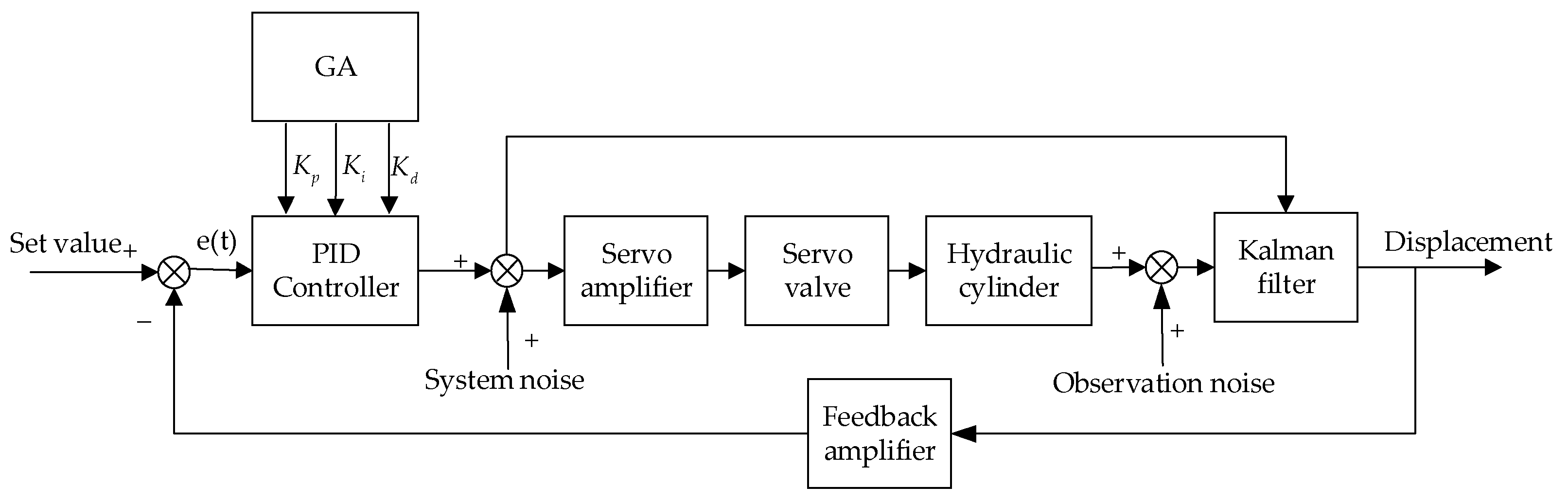
The combination of the Kalman filter and the GA-optimized controller is applied to the position control of the hydraulic servo system. As shown in Figure 7, it can reduce the impact of external interference (such as periodic vibration of servo valve, etc.) on the system.
4. Simulation and Analysis
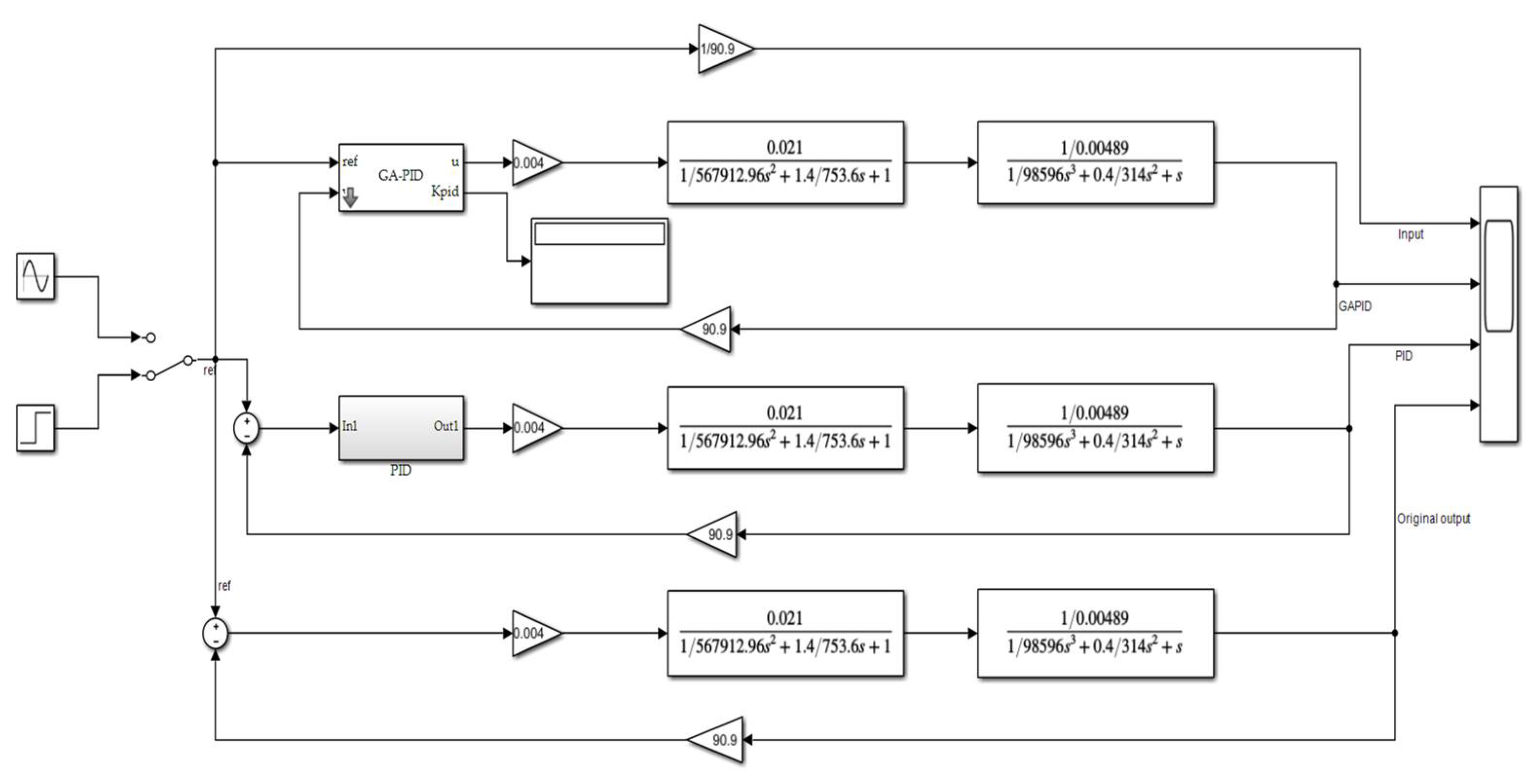
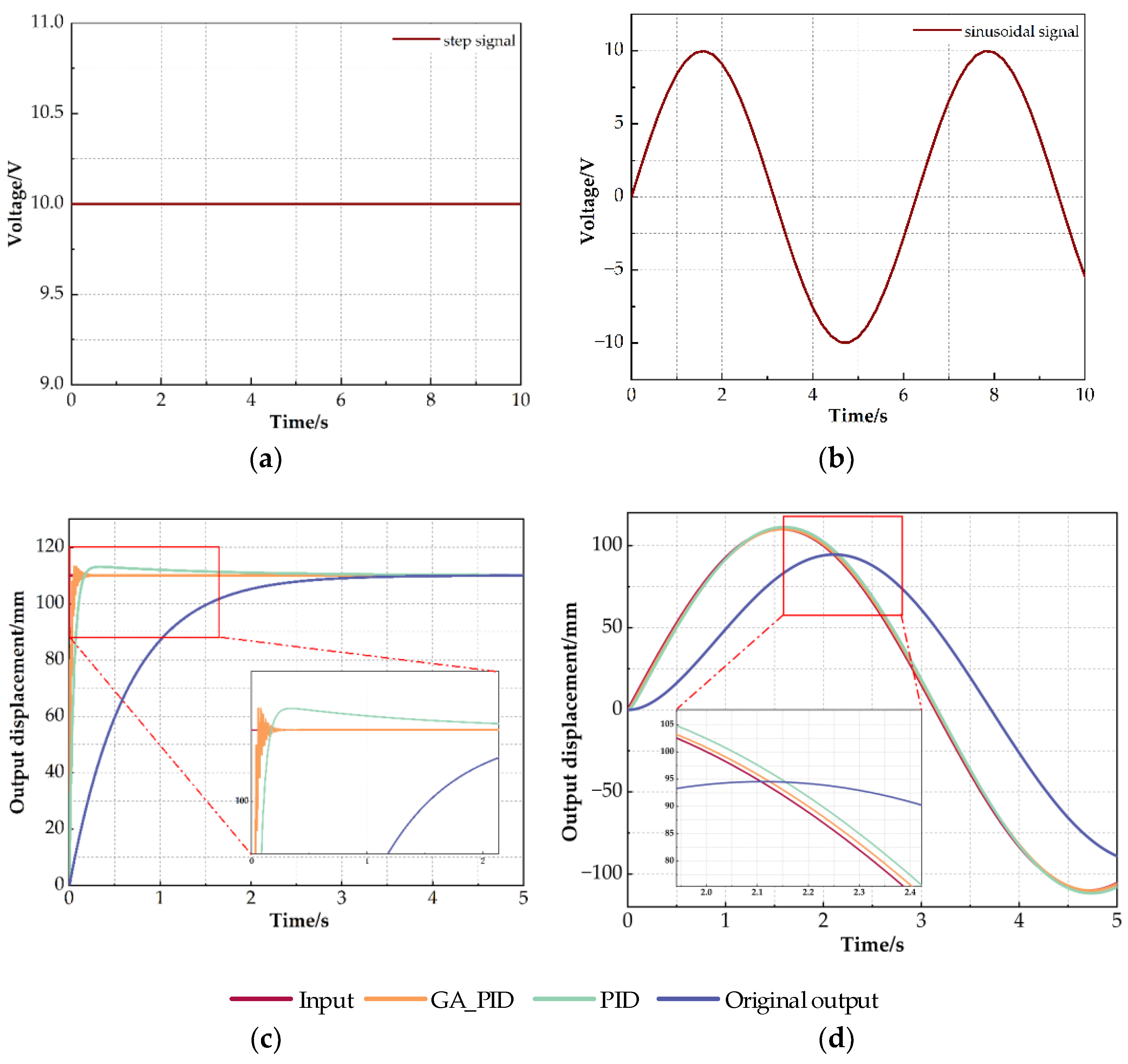
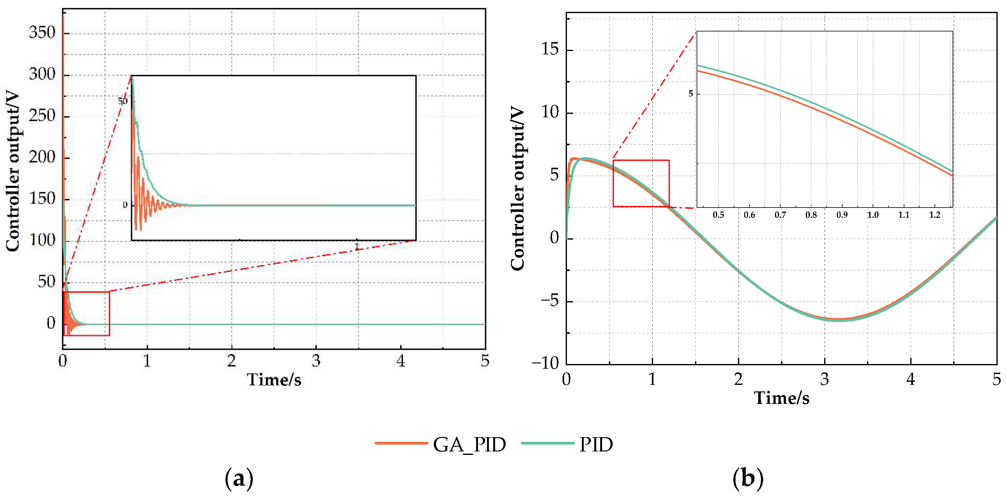
The simulation model of the hydraulic servo system is built in MATLAB/Simulink, and the PID and GA optimized PID control of the system is carried out without interference, as shown in Figure 8. As shown in Figure 9a,b, the step signal and sinusoidal signal are used as the input of the system in turn, and the step response and sinusoidal response under PID control and GA-optimized PID control are compared and analyzed. The system simulation results are shown in Figure 9c,d. The corresponding outputs of the PID control and the GA-optimized PID controller are shown in Figure 10a,b for the case of step and sinusoidal signal inputs, respectively. The selections of the three parameters , , and of the normal PID and GA-optimized PID are shown in Table 2.
As can be seen from Figure 9c, the maximum response of ordinary PID is 0.1132, and the overshoot is 2.9%. The maximum response of PID optimized by GA is 0.1129, and the overshoot is 2.7%. The overshoot of the optimized PID of GA is 0.2% lower than that of ordinary PID. The stable time of the ordinary PID is 1164 s, the adjustment time of PID optimized by GA is 0.063 s, and the adjustment time after optimization is 1101 s better than that before optimization. Taking the time when the output response rises from 10% of the target value to 90% of the target value as the rise time, the rise time of the ordinary PID is 0.0845 s, the rise time of the GA optimized PID is 0.0309 s. The peak time of ordinary PID is 0.248 s. The peak time of PID optimized by GA is 0.061 s. According to the rise time and peak time, under the step signal input, the response speed of the ordinary PID is obviously slower than that of the GA-optimized PID.
As can be seen from Figure 9d, when the control algorithm does not optimize the input sine signal, there is a large amplitude attenuation and phase lag; under the control of PID optimized by PID and GA, the corresponding output displacement of the valve-controlled hydraulic servo system under the sinusoidal signal input has been improved to a certain extent. From the local magnification diagram of the system sinusoidal signal corresponding to the output displacement in Figure 9d, it can be clearly seen that the output response of the sinusoidal signal of the system under the PID control optimized by GA is closer to the input signal of the system in terms of phase and amplitude than that of the ordinary PID. Therefore, the tracking performance of the GA optimized PID is better than that of the ordinary PID. That is, the control performance of the GA optimized is better.
As can be seen from Figure 10a, for the error between the input and output of the system, the PID is close to zero after 0.261 s of regulation, while the system takes 0.227 s with the GA optimized PID regulation, a reduction of 0.034 s over the PID’s regulation time. This shows that the GA-optimized PID has a faster adjustment to error and better tracking performance of the input signal. As can be seen from Figure 10b, the error between the input and output of the system is corrected after both controllers and the error remains stable, whereas the error is zero when passing the mid-point, preventing the accumulation of errors, but the GA-optimized PID correction is faster than the unoptimized PID.
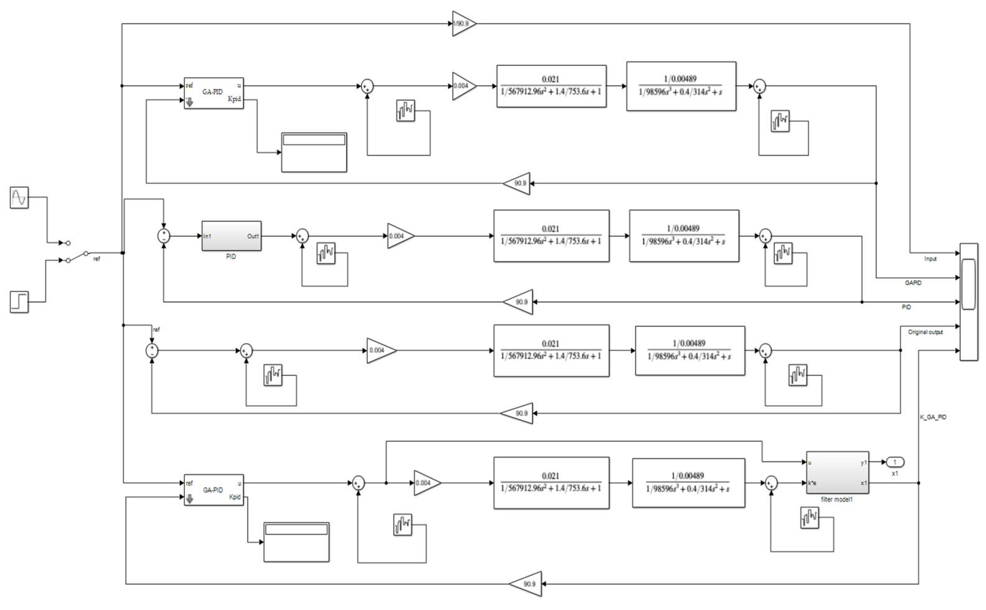
As can be seen from Figure 9c,d, although the output response of the hydraulic servo system after the genetic algorithm-optimized PID controller is somewhat better than the normal PID, the genetic algorithm-optimized PID causes large amplitude fluctuations, which are not allowed in the hydraulic servo system. For the fluctuations caused by the genetic algorithm-optimized PID and the possible external disturbances during the operation of the hydraulic servo system, Kalman filtering is introduced in this paper to deal with them. System noise and observation noise are added to the hydraulic servo system to simulate the hydraulic servo system subjected to external disturbance. A simulation model of the hydraulic servo system is built in Simulink, as shown in Figure 11, to analyze and compare the system immunity under PID, GA-optimized PID control, and GA-optimized PID control after the introduction of the Kalman filter.
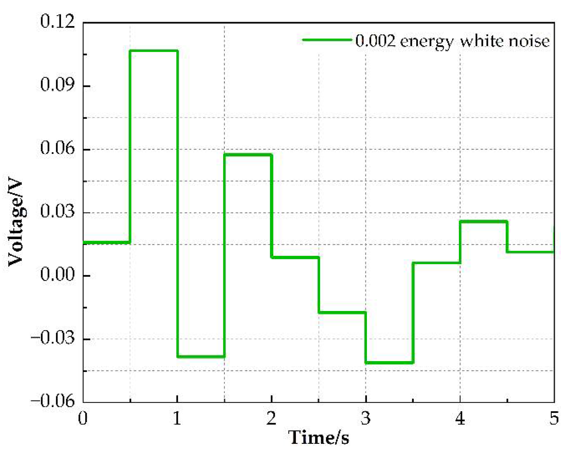
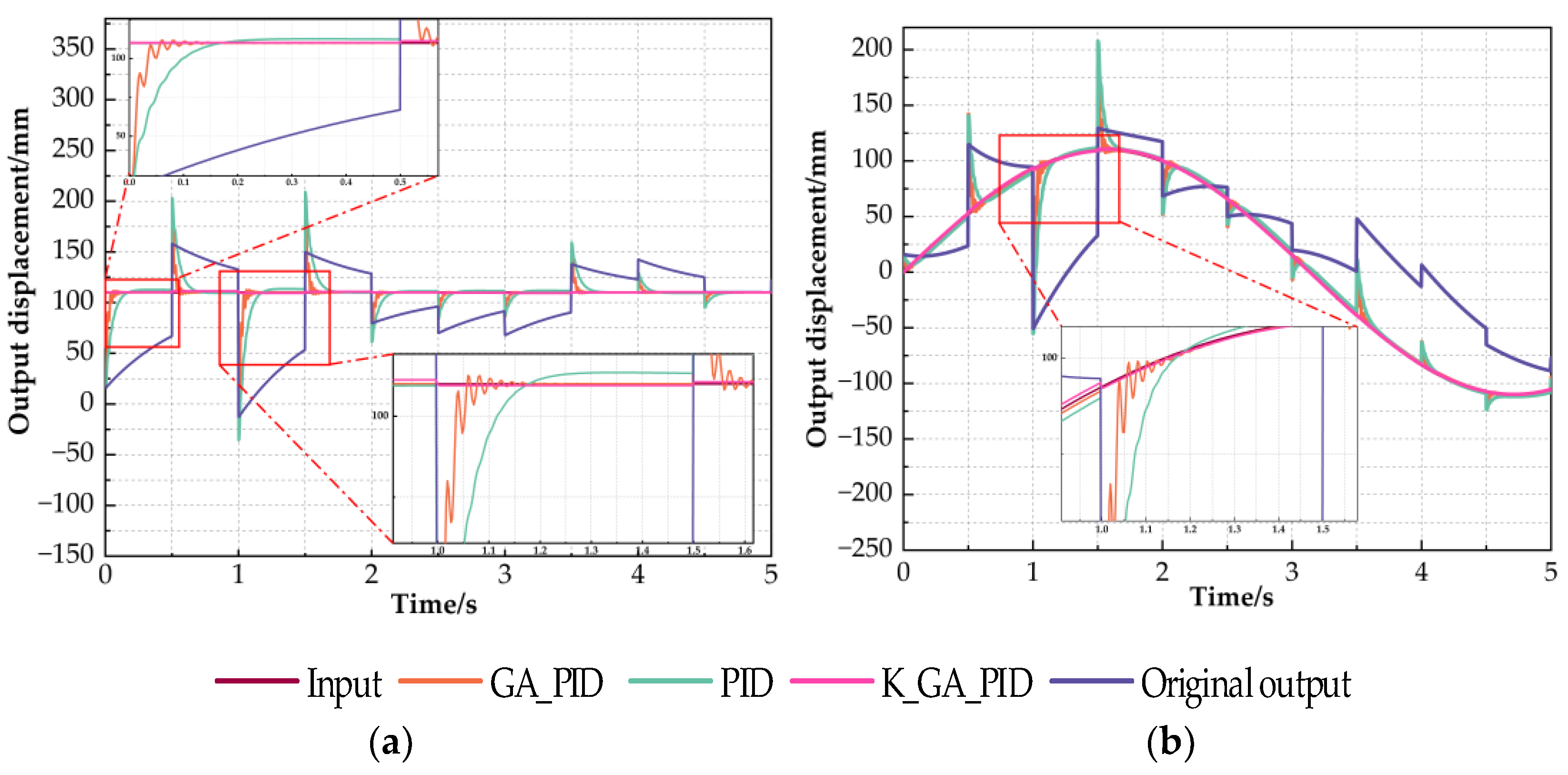
The system noise and observation noise are set to 0.002 energy white noise, as shown in Figure 12. At the same time, the covariance and of system noise and observation noise are set to 1, and the step signal and sinusoidal signal are taken as the input of the system. The step response and sinusoidal response, as shown in Figure 9a,b, under PID control, GA-optimized PID control, and Kalman- and GA-optimized PID control are compared and analyzed. The system simulation results are shown in Figure 13a,b. The corresponding outputs of the PID control and the GA-optimized PID controller are shown in Figure 13a,b for the case of step and sinusoidal signal inputs, respectively.
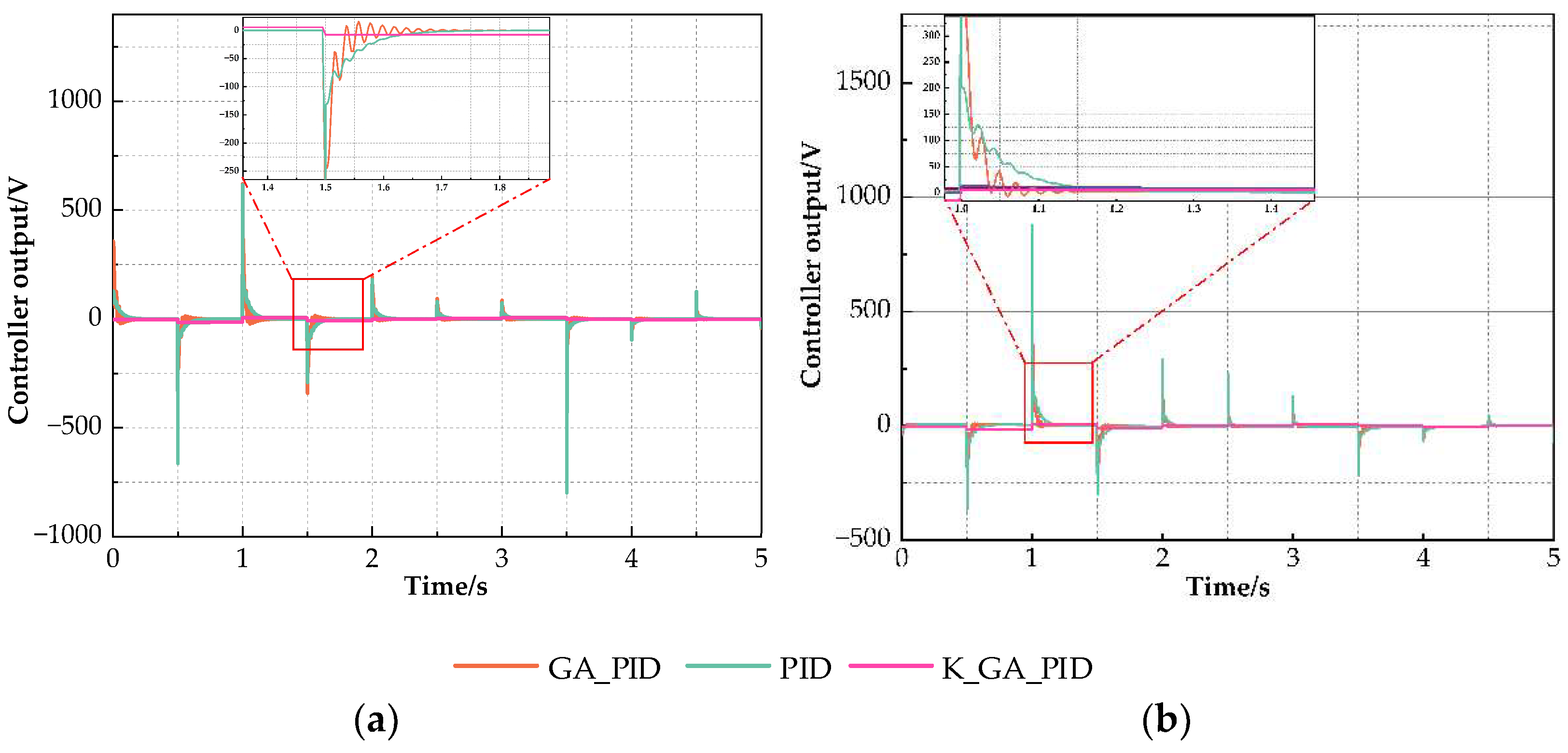
From Figure 13, it can be seen that under the interference of system noise and observation noise with an energy of 0.002, it takes 0.172 s for PID to restore equilibrium and 0.099 s for PID optimized by GA. As can be seen from Figure 14, the PID takes 0.26 s to eliminate the effect of disturbances on the system error when subjected to external disturbances, compared to 0.22 s after GA optimization. At the same time, GA_PID with the Kalman filter module needs almost no time to adjust. It can be seen that the anti-jamming ability of PID is the worst, the anti-jamming ability of PID optimized by GA is better than that of PID, and the anti-jamming performance of GA_PID after Kalman filter is the best, which not only solves the amplitude disturbance of the system caused by the GA optimized PID, but also largely reduces the effect of external disturbance on the system.
5. Conclusions
Aiming at the nonlinearity and uncertainty of the hydraulic servo system, the mathematical model of the valve-controlled hydraulic servo system is constructed. In order to improve the performance of the position control of the hydraulic servo system, a set of PID controllers based on Kalman genetic optimization is designed, and the controller is applied to the established hydraulic servo system for simulation analysis. The results show that the controller designed in this paper can improve the position tracking of the performance of the hydraulic servo system and the anti-interference ability. The GA algorithm is used on the PID controller to realize the tuning of the PID’s three parameters and solve the problem that it is difficult to adjust the PID parameters. The introduction of the Kalman filter on the GA-optimized PID controller solves the amplitude fluctuations in the initial stage caused by the GA-optimized PID while reducing the effect of external disturbances on the system and enhancing the system’s anti-interference capability.
Author Contributions
Conceptualization, Y.-Q.G. and X.-M.Z.; methodology, X.-M.Z.; software, X.-M.Z.; validation, Y.-Y.S., Y.-N.W. and G.C.; formal analysis, X.-M.Z.; investigation, Y.-N.W.; resources, Y.-Q.G.; data curation, X.-M.Z.; writing—original draft preparation, X.-M.Z.; writing—review and editing, Y.-Q.G.; visualization, X.-M.Z.; supervision, Y.-Q.G.; project administration, Y.-Q.G.; funding acquisition, Y.-Q.G. All authors have read and agreed to the published version of the manuscript.
Funding
This work was supported by the National Key R&D Programs of China under Grant 2019YFE0121900, the National Natural Science Foundation of China under Grant 51878355, and the National Natural Science Foundation of China Key Projects under Grant 52130807.
Institutional Review Board Statement
Not applicable.
Informed Consent Statement
Not applicable.
Data Availability Statement
Not applicable.
Conflicts of Interest
The authors declare no conflict of interest.
References
- Ye, Y.; Yin, C.-B.; Gong, Y.; Zhou, J.-j. Position control of nonlinear hydraulic system using an improved PSO based PID controller. Mech. Syst. Signal Proc. 2017, 83, 241–259. [Google Scholar] [CrossRef]
- Xing, Z.-Y.; Gao, Q.; Jia, L.-M.; Wu, Y.-Y. Modelling and Identification of Electrohydraulic System and Its Application. IFAC Proc. Vol. 2008, 41, 6446–6451. [Google Scholar] [CrossRef] [Green Version]
- Kalyoncu, M.; Haydim, M. Mathematical modelling and fuzzy logic based position control of an electrohydraulic servosystem with internal leakage. Mechatronics 2009, 19, 847–858. [Google Scholar] [CrossRef]
- Zheng, J.-M.; Zhao, S.-D.; Wei, S.-G. Application of self-tuning fuzzy PID controller for a SRM direct drive volume control hydraulic press. Control Eng. Pract. 2009, 17, 1398–1404. [Google Scholar] [CrossRef]
- Yao, J.; Jiao, Z. Electrohydraulic Positioning Servo Control Based on Its Adaptive Inverse Model. In Proceedings of the 6th IEEE Conference on Industrial Electronics and Applications (ICIEA), Beijing, China, 21–23 June 2011; pp. 1698–1701. [Google Scholar] [CrossRef]
- Li, X.; Yao, J.; Zhou, C. Output feedback adaptive robust control of hydraulic actuator with friction and model uncertainty compensation. J. Frankl. Inst. 2017, 354, 5328–5349. [Google Scholar] [CrossRef]
- Shen, W.; Wang, J.; Huang, H.; He, J. Fuzzy sliding mode control with state estimation for velocity control system of hydraulic cylinder using a new hydraulic transformer. Eur. J. Control 2018, 48, 104–114. [Google Scholar] [CrossRef]
- Knohl, T.; Unbehauen, H. Adaptive position control of electrohydraulic servo systems using ANN. Mechatronics 2000, 10, 127–143. [Google Scholar] [CrossRef]
- Bao, R.; Wang, Q.; Wang, T. Energy-Saving Trajectory Tracking Control of a Multi-Pump Multi-Actuator Hydraulic System. IEEE Access 2020, 8, 179156–179166. [Google Scholar] [CrossRef]
- Zhang, S.; Chen, T.; Minav, T.; Cao, X.; Wu, A.; Liu, Y.; Zhang, X. Position Soft-Sensing of Direct-Driven Hydraulic System Based on Back Propagation Neural Network. Actuators 2021, 10, 322. [Google Scholar] [CrossRef]
- Nguyen, M.; Dao, H.; Ahn, K. Active Disturbance Rejection Control for Position Tracking of Electro-Hydraulic Servo Systems under Modeling Uncertainty and External Load. Actuators 2021, 10, 20. [Google Scholar] [CrossRef]
- Zhang, Y.; Li, K.; Cai, M.; Wei, F.; Gong, S.; Li, S.; Lv, B. Establishment and Experimental Verification of a Nonlinear Position Servo System Model for a Magnetically Coupled Rodless Cylinder. Actuators 2022, 11, 50. [Google Scholar] [CrossRef]
- Chang, W.-D. Nonlinear CSTR control system design using an artificial bee colony algorithm. Simul. Model. Pract. Theory 2013, 31, 1–9. [Google Scholar] [CrossRef]
- Wang, H.; Du, H.; Cui, Q.; Song, H. Artificial bee colony algorithm based PID controller for steel stripe deviation control system. Sci. Prog. 2022, 105, 1–22. [Google Scholar] [CrossRef] [PubMed]
- Feng, H.; Ma, W.; Yin, C.; Cao, D. Trajectory control of electro-hydraulic position servo system using improved PSO-PID controller. Autom. Constr. 2021, 127, 103722. [Google Scholar] [CrossRef]
- Wang, Z.; Wang, Q.; He, D.; Liu, Q.; Zhu, X.; Guo, J. An Improved Particle Swarm Optimization Algorithm Based on Fuzzy PID Control. In Proceedings of the 4th International Conference on Information Science and Control Engineering (ICISCE), Changsha, China, 21–23 July 2017; pp. 835–839. [Google Scholar] [CrossRef]
- Shutnan, W.A.; Abdalla, T.Y. Artificial Immune system based Optimal Fractional Order PID Control Scheme for Path Tracking of Robot manipulator. In Proceedings of the International Conference on Advances in Sustainable Engineering and its Application (ICASEA), Wasit, Iraq, 14–15 March 2018. [Google Scholar] [CrossRef]
- Guo, W.; Wang, W.; Qiu, X. An Improved Generalized Predictive Control Algorithm Based on PID. In Proceedings of the International Conference on Intelligent Computation Technology and Automation, Changsha, China, 20–22 October 2008. [Google Scholar] [CrossRef]
- Odili, J.B.; Kahar, M.N.M.; Noraziah, A. Parameters-tuning of PID controller for automatic voltage regulators using the African buffalo optimization. PLoS ONE 2017, 12, e0175901. [Google Scholar] [CrossRef] [Green Version]
- Bingul, Z.; Karahan, O. A novel performance criterion approach to optimum design of PID controller using cuckoo search algorithm for AVR system. J. Frankl. Inst. 2018, 355, 5534–5559. [Google Scholar] [CrossRef]
- Loucif, F.; Kechida, S.; Sebbagh, A. Whale optimizer algorithm to tune PID controller for the trajectory tracking control of robot manipulator. J. Braz. Soc. Mech. Sci. Eng. 2019, 42, 1. [Google Scholar] [CrossRef]
- Xue, J.-J.; Wang, Y.; Li, H.; Meng, X.-F.; Xiao, J.-Y. Advanced Fireworks Algorithm and Its Application Research in PID Parameters Tuning. Math. Probl. Eng. 2016, 2016, 2534632. [Google Scholar] [CrossRef] [Green Version]
- Gao, X.; Shi, D.; Mu, Z. PID Optimization of Motion Servo Control System Based on Improved Artificial Fish Swarm Algorithm. In Proceedings of the Chinese Automation Congress (CAC), Xian, China, 30 November–2 December 2018. [Google Scholar] [CrossRef]
- Liu, H.; Li, Y.; Zhang, Y.; Chen, Y.; Song, Z.; Wang, Z.; Zhang, S.; Qian, J. Intelligent tuning method of PID parameters based on iterative learning control for atomic force microscopy. Micron 2018, 104, 26–36. [Google Scholar] [CrossRef]
- Chen, L. The Optimization of PID Control Strategy in VAV System Based on Bacterial Foraging Algorithm. In Proceedings of the 19th International Conference on Network-Based Information Systems (NBiS), Ostrava, Czech Republic, 7–9 September 2016. [Google Scholar] [CrossRef]
- Liu, X.; Shi, Y.; Xu, J. Parameters Tuning Approach for Proportion Integration Differentiation Controller of Magnetorheological Fluids Brake Based on Improved Fruit Fly Optimization Algorithm. Symmetry 2017, 9, 109. [Google Scholar] [CrossRef] [Green Version]
- Veerasamy, G.; Kannan, R.; Siddharthan, R.; Muralidharan, G.; Sivanandam, V.; Amirtharajan, R. Integration of genetic algorithm tuned adaptive fading memory Kalman filter with model predictive controller for active fault-tolerant control of cement kiln under sensor faults with inaccurate noise covariance. Math. Comput. Simul. 2021, 191, 256–277. [Google Scholar] [CrossRef]
- Xu, Z.-D.; Guo, Y.-F.; Wang, S.-A.; Huang, X.-H. Optimization analysis on parameters of multi-dimensional earthquake isolation and mitigation device based on genetic algorithm. Nonlinear Dyn. 2013, 72, 757–765. [Google Scholar] [CrossRef]
- Ouyang, Z.L.; Zou, Z.J. Nonparametric modeling of ship maneuvering motion based on Gaussian process regression optimized by genetic algorithm. Ocean. Eng. 2021, 238, 109699. [Google Scholar] [CrossRef]
- Xu, Z.-D.; Huang, X.-H.; Xu, F.-H.; Yuan, J. Parameters optimization of vibration isolation and mitigation system for precision platforms using non-dominated sorting genetic algorithm. Mech. Syst. Signal Process. 2019, 128, 191–201. [Google Scholar] [CrossRef]
- Chen, W.; Wei, Q.; Zhang, Y. Research on anti-interference of ROV based on particle swarm optimization fuzzy PID. In Proceedings of the Chinese Automation Congress (CAC), Shanghai, China, 6–8 November 2020. [Google Scholar] [CrossRef]
- Chao, C.-T.; Sutarna, N.; Chiou, J.-S.; Wang, C.-J. An Optimal Fuzzy PID Controller Design Based on Conventional PID Control and Nonlinear Factors. Appl. Sci. 2019, 9, 1224. [Google Scholar] [CrossRef] [Green Version]
- Wu, T.-Y.; Jiang, Y.-Z.; Su, Y.-Z.; Yeh, W.-C. Using Simplified Swarm Optimization on Multiloop Fuzzy PID Controller Tuning Design for Flow and Temperature Control System. Appl. Sci. 2020, 10, 8472. [Google Scholar] [CrossRef]
- Xu, F.-X.; Liu, X.-H.; Chen, W.; Zhou, C.; Cao, B.-W. Fractional order PID control for steer-by-wire system of emergency rescue vehicle based on genetic algorithm. J. Central South Univ. 2019, 26, 2340–2353. [Google Scholar] [CrossRef]
- Agrebi, H.; Benhadj, N.; Chaieb, M.; Sher, F.; Amami, R.; Neji, R.; Mansfield, N. Integrated Optimal Design of Permanent Magnet Synchronous Generator for Smart Wind Turbine Using Genetic Algorithm. Energies 2021, 14, 4642. [Google Scholar] [CrossRef]
- Al-Maliki, A.Y.; Iqbal, K. FLC-Based PID Controller Tuning for Sensorless Speed Control of DC Motor. In Proceedings of the 19th IEEE International Conference on Industrial Technologies (ICIT), Lyon, France, 19–22 February 2018. [Google Scholar] [CrossRef]
- Li, H.; Yu, Q. The Wire Beltline Diameter ACO-KF-PID Control Research. In Proceedings of the Prognostics and System Health Management Conference (PHM-Chengdu), Chengdu, China, 19–21 October 2016. [Google Scholar] [CrossRef]
- Wu, H.; Chen, S.-X.; Yang, B.-F.; Chen, K. Robust cubature Kalman filter target tracking algorithm based on genernalized M-estiamtion. Acta Phys. Sin. 2015, 64, 218401. [Google Scholar] [CrossRef]
- Golestan, S.; Guerrero, J.M.; Vasquez, J.C.; Abusorrah, A.M.; Al-Turki, Y.A. Single-Phase FLLs Based on Linear Kalman Filter, Limit-Cycle Oscillator, and Complex Bandpass Filter: Analysis and Comparison with a Standard FLL in Grid Applications. IEEE Trans. Power Electron. 2019, 34, 11774–11790. [Google Scholar] [CrossRef]
- Chen, W.-D.; Liu, Y.-L.; Zhu, Q.-G.; Chen, Y. Fuzzy adaptive extended Kalman filter SLAM algorithm based on the improved wild geese PSO algorithm. Acta Phys. Sin. 2013, 62, 170506. [Google Scholar] [CrossRef]
Figure 1.
Schematic diagram of valve-controlled hydraulic servo system.

Figure 2.
Valve-controlled hydraulic cylinder schematic.

Figure 3.
Control flow chart of valve-controlled hydraulic cylinder.

Figure 4.
Hydraulic servo system PID control.

Figure 5.
PID Controller optimized by genetic algorithm.

Figure 6.
Schematic diagram of GA-tuning PID parameters.

Figure 7.
PID position control of hydraulic servo system based on Kalman genetic optimization.

Figure 8.
Optimization of PID simulation diagram by GA.

Figure 9.
Simulation results of the system without noise. (a) Step signal input; (b) Sinusoidal signal; (c) System simulation results under step signal input; (d) System simulation results under sinusoidal signal input.
Figure 9.
Simulation results of the system without noise. (a) Step signal input; (b) Sinusoidal signal; (c) System simulation results under step signal input; (d) System simulation results under sinusoidal signal input.

Figure 10.
Output of PID and GA-optimized PID controllers. (a) Controller output under step signal input; (b) Controller output under sinusoidal signal input.
Figure 10.
Output of PID and GA-optimized PID controllers. (a) Controller output under step signal input; (b) Controller output under sinusoidal signal input.

Figure 11.
System Simulation Diagram of Kalman filter-optimized genetic PID.

Figure 12.
0.002 energy white noise.

Figure 13.
System simulation results under 0.002 energy white noise. (a) System simulation results under step signal input; (b) System simulation results under sinusoidal signal input.
Figure 13.
System simulation results under 0.002 energy white noise. (a) System simulation results under step signal input; (b) System simulation results under sinusoidal signal input.

Figure 14.
Output of PID and GA-optimized PID controllers under external disturbances. (a) Controller output under step signal input; (b) Controller output under sinusoidal signal input.
Figure 14.
Output of PID and GA-optimized PID controllers under external disturbances. (a) Controller output under step signal input; (b) Controller output under sinusoidal signal input.


Table 1.
Hydraulic cylinder and servo valve parameters.
| Parameters | Numerical Value |
|---|---|
| Work trip | |
| Hydraulic cylinder bore | |
| Piston rod bore | |
| Valve rated current | |
| Total compression volume () | |
| Load Quality () | |
| Effective piston area () | |
| Servo valve flow gain () | |
| Effective bulk modulus of elasticity () | |
| Oil supply pressure () | 2.1 Mpa |
| Total flow pressure coefficient () | |
| Hydraulic natural frequency () | |
| Hydraulic damping ratio () | 0.2 |
| Natural frequency of servo valve () | |
| Damping ratio of servo valve () | 0.7 |
Table 2.
Parameter values of ordinary PID and GA-optimized PID.
| Parameters | PID | GA-PID |
|---|---|---|
| 20 | 39.72 | |
| 1 | 0.9914 | |
| 0.1 | 0.033 |
Publisher’s Note: MDPI stays neutral with regard to jurisdictional claims in published maps and institutional affiliations. |
© 2022 by the authors. Licensee MDPI, Basel, Switzerland. This article is an open access article distributed under the terms and conditions of the Creative Commons Attribution (CC BY) license (https://creativecommons.org/licenses/by/4.0/).
Share and Cite
MDPI and ACS Style
Guo, Y.-Q.; Zha, X.-M.; Shen, Y.-Y.; Wang, Y.-N.; Chen, G. Research on PID Position Control of a Hydraulic Servo System Based on Kalman Genetic Optimization. Actuators 2022, 11, 162. https://0-doi-org.brum.beds.ac.uk/10.3390/act11060162
AMA Style
Guo Y-Q, Zha X-M, Shen Y-Y, Wang Y-N, Chen G. Research on PID Position Control of a Hydraulic Servo System Based on Kalman Genetic Optimization. Actuators. 2022; 11(6):162. https://0-doi-org.brum.beds.ac.uk/10.3390/act11060162
Chicago/Turabian StyleGuo, Ying-Qing, Xiu-Mei Zha, Yao-Yu Shen, Yi-Na Wang, and Gang Chen. 2022. "Research on PID Position Control of a Hydraulic Servo System Based on Kalman Genetic Optimization" Actuators 11, no. 6: 162. https://0-doi-org.brum.beds.ac.uk/10.3390/act11060162
Note that from the first issue of 2016, this journal uses article numbers instead of page numbers. See further details here.