
Trajectory Generation Method for Serial Robots in Hybrid Space Operations

1
College of Computer and Control Engineering, Northeast Forestry University, Harbin 150036, China
2
School of Mechanical Engineering, Shanghai Jiao Tong University, Shanghai 200240, China
3
College of Mechanical Engineering, Donghua University, Shanghai 201600, China
*
Author to whom correspondence should be addressed.
Actuators 2024, 13(3), 108; https://0-doi-org.brum.beds.ac.uk/10.3390/act13030108
Submission received: 2 February 2024
/
Revised: 3 March 2024
/
Accepted: 6 March 2024
/
Published: 8 March 2024
(This article belongs to the Special Issue Motion Planning and Control of Robot Systems)
Abstract
:The hybrid space of robots is divided into task space and joint space, with task space focused on trajectory-tracking accuracy, while joint space considers dynamic responsiveness and synchronization. Therefore, the robot-motion control systems need to effectively integrate both aspects, ensuring precision in task trajectory while promptly responding to unforeseen environmental events. Hence, this paper proposes an online trajectory-generation method for robots in both joint and task spaces. In task space, a planning approach is presented for high-precision NURBS curves. The global NURBS curve is segmented into several rational Bezier curves, establishing local coordinate systems for control points. This ensures that all local control points meet the chord error constraint, guaranteeing trajectory accuracy. To address the feed rate dynamic planning issue for segmented curves, an improved online S-shape feed-rate scheduling framework is introduced. This framework dynamically adjusts the current execution speed to meet task requirements. In joint space, an offline velocity planning based on a time synchronization scheme and a multi-dimensional synchronization technique based on the principle of spatial-coordinate system projection are proposed. Building upon the offline scheme, it allows for the modification of the target state for any sub-dimension during the motion process, with the remaining dimensions adapting accordingly. Simulation and experimentation demonstrate that the two proposed online trajectory generations for robot motion spaces, while ensuring task trajectory accuracy, effectively handle external unexpected events. They ensure joint synchronization and smoothness, carrying significant practical implications and application value for the stability of robot systems.
1. Introduction
The challenges and demands faced by the motion-control system of robots in handling both joint space and task space underscore the elevated requirements for modern robotic applications [1]. The integration of joint space and task space, coupled with the simultaneous consideration of dynamic responsiveness, synchronization, and trajectory-tracking accuracy, is paramount for achieving efficient, flexible, and secure robot operations [2,3]. In the task space, trajectory-tracking accuracy refers to the robot’s end-effector’s capacity to precisely follow the specified path during task execution. This precision is particularly crucial for applications requiring high-precision manipulation, such as precision assembly and medical surgeries [4,5]. In joint space, dynamic responsiveness denotes the robot system’s rapid adaptability to external disturbances or changes, a critical factor in ensuring the stability and accuracy of the robot in real-time operations [6,7]. Synchronization involves the coordinated movement among the various joints of the robot, ensuring their collaborative action during task execution and avoiding discrepancies or asynchronies in the motion process [8]. By comprehensively addressing the requirements of joint space and task space, the robot motion control systems can better adapt to diverse and dynamic work environments, achieving high-precision and efficient task execution.
The task space imposes strict operational paths with heightened precision trajectory demands. Therefore, the initial consideration involves controlling errors in the task path, followed by imposing constraints on the trajectory. Taking the common example of spline paths in machining operations within the task space, although [9,10] achieves a positional and orientational smoothing of the paths using task space splines, this fails to account for the contour error requirements in the path. As such, it cannot be effectively applied to tasks with precision constraints at the end-effector. To process complex spatial free-form curves like NURBS [11], robots require high-precision interpolation capabilities. Initially, offline programming is carried out to acquire curve control points that satisfy the contour error constraint. Next, the curve is sampled offline, sectioned based on curvature extremes, and lastly segmented curve interpolation is executed. Low-speed processing hardly affects the accuracy of the cutting path shape. Nevertheless, high-speed processing results in a significant chord error, particularly in regions with high curvatures. Existing commercial numerical control systems are equipped with advanced look-ahead capabilities. Similarly, high-end motion-control cards are equipped with look-ahead algorithms. Most precision error control strategies, however, are developed specifically for numerical-control machine tools. Most of the currently used approaches in China and other countries comprise constraining the machining trajectory in the task space directly to comply with the chord error constraint during the process. Some achievements were made in calculating the chord error of the path. The equation parameter changing step-size method [12] has the benefits of simplicity and high efficiency, while the Hausdorff distance method [13] can characterize the distance relationship between expected and actual paths. Currently, discrete estimation such as the second-order tangent circle method [14,15] is primarily used. Moreover, in the field of robot machining, it is imperative to employ discrete curvature scanning techniques for the segmentation of the overall curve into multiple sub-curves. A common approach to determine the critical points of high curvature sub-curves and limit the chord error is based on curvature-adaptive interpolation algorithm [16]. Nevertheless, this method involves complicated calculations resulting in low efficiency, and there is no practical approach in dividing the curve between two curvature extremes to achieve specific accuracy requirements.
Currently, trajectory planning and interpolation for NURBS curves are executed separately [17,18]. Fan et al. [19] introduced a planning method for S-shape feed-rate scheduling, dividing the motion into 15 segments. The scheme’s major issue was its excessive computational complexity, which made it intricate to develop and sustain. Song et al. [20] proposed an S-shape feed-rate-scheduling algorithm that elevates the standard third order to the fourth order, providing a continuous jerk. However, this also augments the number of motion segments by up to 15, significantly complicating the process and requiring a long offline planning period. A new framework for controlling S-shape feed-rate scheduling was created by Li et al. [21]. By combining the advantages of traditional S-shape feed-rate scheduling with the continuous differentiability of sine and cosine functions, they added a sinusoidal start and stop, in addition to an S-shape feed rate scheduling smoothing section. Consequently, the new framework significantly decreased the vibration resulting from the conventional S-shape feed rate scheduling. Nevertheless, this algorithm fails to sustain optimal acceleration, results in non-optimal time, and produces acceleration jumps at endpoints. Ref. [22] delved into examining the properties of asymmetric motion in the context of feed-rate planning. While the algorithm is straightforward, it fails to maintain constant maximum acceleration and jerk due to the use of sine curves, causing a reduction in time efficiency. After trajectory planning comes the work of NURBS curve interpolation.
In joint space, there is no precision metric for path accuracy; the requirement is solely for reachable positions while considering constraints such as time optimality and kinematic limits during the process [23]. Currently, time-optimal path planning in robotics primarily falls into two categories: optimization-based approaches [24,25,26] and numerical integration-based approaches [27,28]. The advantage of convex optimization methods lies in achieving globally optimal path solutions, obtaining optimal states at each discrete path points. However, the downside is the substantial computational load, necessitating robust hardware and offline calculations for practical use. Similarly, numerical integration-based methods also require offline computation and continuous iterative optimization, with comparatively complex formulas, adding to the implementation complexity. Both approaches involve obtaining discrete states, necessitating further integration with interpolation algorithms to generate executable trajectories. This creates a situation where discrete point constraints are reachable, and the intermediary process heavily relies on the choice of interpolation algorithms, potentially leading to over-constraint issues. In addition, with the development of artificial intelligence technology, there has been a growing body of research utilizing artificial intelligence methods for generating robot motion trajectories. Ref. [29] introduces a robot obstacle-avoidance trajectory-generation technique based on policy gradient reinforcement learning. The core of this approach involves combining a Deep Deterministic Policy Gradient (DDPG) algorithm with a Hindsight Experience Replay (HER) algorithm, successfully applied to obstacle environments for 6-DOF manipulator obstacle-avoidance trajectory control. Ref. [30] presents a motion-planning algorithm for robot manipulators using a twin delayed deep deterministic policy gradient (TD3), a reinforcement learning algorithm tailored to MDP with continuous action. Additionally, hindsight experience replay (HER) is employed in the TD3 to enhance sample efficiency. However, the paper only includes simulation verification for 2-DOF and 3-DOF manipulators, lacking experimental validation for the multi-DOF manipulator. Regarding multidimensional synchronization techniques in offline velocity planning, three main approaches are considered. One involves constructing time-dependent polynomials for time-constrained synchronous planning, such as cubic, quintic, or heptic polynomials, requiring only specified time constraints to fit synchronized motion trajectories. While straightforward, this method fails to achieve smooth transitional phases, such as in tasks requiring constant-speed trajectories. Moreover, with an increase in polynomial order, the likelihood of the Runge phenomenon rises, resulting in smooth yet significantly oscillatory motions, particularly impactful for serial manipulators with frequent speed fluctuations. The second approach is the time scaling technique, based on independent planning for each dimension, determining the longest dimension in motion time and proportionally scaling the others based on this maximum dimension. This achieves synchronous motion for point-to-point multidimensional movement, allowing the fastest realization of arbitrary point-to-point transitions. However, the downside lies in velocity changes caused by the alteration of interpolation time factors for shorter dimensions, making subsequent multi-path velocity planning challenging. Ref. [31] offers a solution by coupling multiple axes in task space for synchronization. The third approach involves real-time joint space velocity planning, as presented in [6,32], abandoning the pursuit of time optimality in favor of ensuring velocity smoothness. For multi-joint synchronization, it utilizes time-constrained planning for each joint’s velocity planning. The approach then employs the maximum duration as a constraint, re-planning the remaining joints to ensure temporal synchronization. Due to its reliance on analytical equation calculations, it may face challenges in planning failure when given targets violate S-shape velocity profiles.
In the task space, the existing technique for curve discretization employs an iso-parametric approach. However, in areas with high curvature, this method produces significant errors resulting in non-controllable overall error. As such, even small parameter changes lead to significant changes in the curvature plot. NURBS interpolation calculations contain errors, resulting in imprecise tails of the curve. Additionally, Taylor’s expansion simplification omits higher-order terms, causing truncation errors. These errors make it challenging to achieve high-precision curve planning. Iterative calculations during trajectory planning lead to reduced efficiency. For segmented curves, dynamic feed-rate scheduling with fixed or variable arc lengths is not supported in task space. In joint space, the first consideration is to achieve smooth synchronized velocity planning for multiple joints to reduce end-effector jitter. Building upon this foundation, it is essential to address the robot’s ability to handle unexpected events in any state. However, many existing solutions overlook how velocity planning should be carried out in arbitrary states. Moreover, velocity planning comes with predefined constraint conditions, and if the initial conditions do not meet these constraints, either planning failure or unacceptable velocity and acceleration discontinuities may occur. Simultaneously, the challenge of synchronizing multiple dynamic joints persists, constituting a technical difficulty in both offline and online trajectory-generation techniques for multi-degree-of-freedom manipulator motion control.
To address the challenges arising in the aforementioned mixed-space operations, particularly in the task space operations, this paper proposes a method for calculating the curve chord error based on the convex hull property of splines. The entire NURBS curve is segmented into multiple Bezier curves using a node-insertion technique, and a local frame is created for each curve segment. The distance between the control point and the curve is calculated, and only distances fulfilling chord error constraint are required using the convex hull property of the spline curve. Then, an error compensation and vibration-suppression algorithm for spatial curve-displacement online feed-rate scheduling is proposed, based on the existing online feed-rate scheduling, to suit online processing tasks; in the joint space, a multi-dimensional synchronization technique is proposed based on the principle of spatial coordinate system projection. Building upon offline synchronization planning, the online synchronization technique allows for the modification of target states in any sub-dimension during the motion process, with the remaining dimensions adapting dynamically for compatibility. This approach proves effective for enabling robots to respond swiftly to unforeseen events.
The remaining sections of this paper are structured as subheadings. Section 2 introduces a chord error control algorithm for segmenting NURBS curves in task space. An improved online trajectory-planning algorithm is proposed in Section 3. Additionally, Section 4 introduces joint motion-synchronization techniques, encompassing both offline and online modes, thereby rendering them applicable for the synchronized trajectory generation in serial robot systems. The simulations and experiments in support of the proposed methods are conducted in Section 5. Finally, Section 6 presents the conclusions.
2. Discretization of NURBS Curves Based on Chord Error Constraints
In flat machining, CAM systems are commonly used to generate tool paths, and curve feed-rate scheduling and interpolation are executed by splicing small line segments and transition connections. If there is a discontinuity in tangential and curvature in the linear tool path, it may result in poor machining quality that fails to meet high precision requirements. To address this issue, cubic NURBS curves are used in this study to describe the path in task space. The expression for the NURBS curve’s rational basis function is presented below:
where , are the control points, are the weights, is the degree and is the non-uniform knot vector. are the B-spline basis functions.
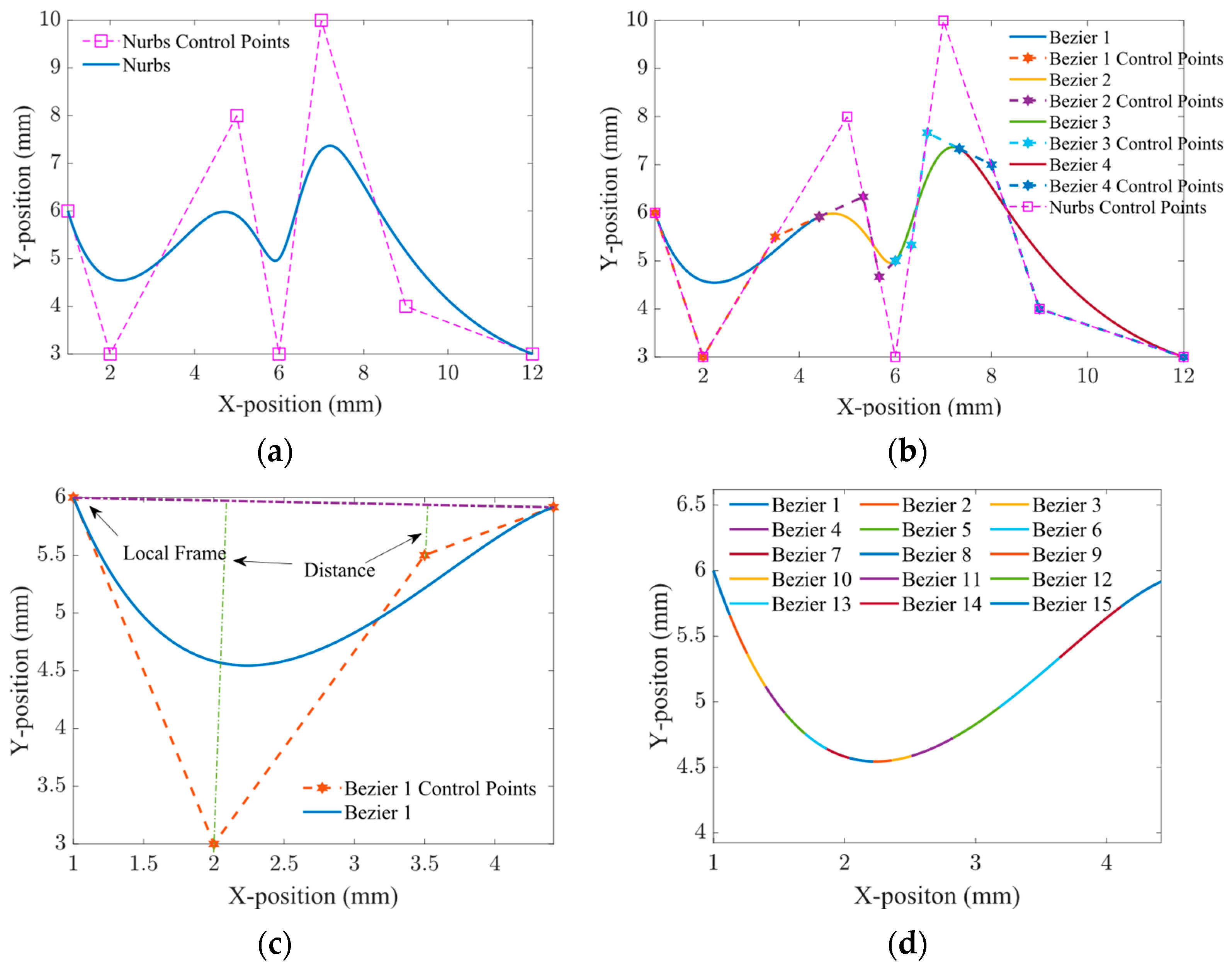
When inserted, nodes [33] generate new control points according to a specified rule, and the original spline can be reconstructed as a new local Bezier curve while retaining its original shape. This characteristic has been proven to be advantageous for partitioning the spline into Bezier curve segments, thereby enhancing the efficiency and simplicity of curve control for segmented Bezier curves. By using the technique, the NURBS curve can be segmented into multiple Bezier curves. The convex hull property of the spline curve is employed, and it is only necessary to ensure that the distance between the control points and the local frame is less than the specified chord error threshold to comply with the curve constraint. Thus, new control points are continually generated, and their projection distance to the local frame is computed. The original curve is bisected until the chord error satisfies the constraints, as illustrated in Figure 1.
Segmenting NURBS curves into multiple Bezier curves is achieved by utilizing the projection distance in the local coordinate system of control points as the chord error. If the constraints are not met, the bisection technique is iteratively employed to add new control points. The process involves continuously recalculating the projection distance of all control points in the local coordinate system for the newly generated curve until the constraints are satisfied. Table 1 presents the results of the initial segmentation in this study, which involves the direct use of knot-insertion techniques. Algorithm 1 outlines the entire segmentation process.
| Algorithm 1: Discretization of NURBS curves based on chord error constraints |
| Input: NURBS curve’s parameters, the chord error constraint δ Output: A collection of Bezier curves satisfying the chord error constraint 1: knot insertion → NURBS to Bezier curve Ci; 2: for i = 1 to the number of Ci curve do 3: do curve Ci projection distance in the local coordinate system of control points; 4: if max(distance) > δ then 5: do knot insertion for Ci and go to step 3; 6: else 7: return Ci; 8: end 9: end |
The proposed method is systematically compared with other methods mentioned in this paper (M.L. [16], X.D. [34], W.L. [35]). Table 2 compares different characteristics. Due to the precision of the test data, the times recorded in the table represent approximate values within specified time intervals. The other methods are based on open-loop arch height error-constrained curve-segmentation methods, which do not incur time consumption but result in larger arch-height errors and lower trajectory-contour accuracy. On the other hand, the method proposed in this paper belongs to a closed-loop iterative algorithm. Although it incurs some time consumption compared to other algorithms in terms of computational efficiency, it achieves relatively high computational efficiency due to its reliance on convex hull geometry-based segmentation and iteration. This approach avoids the complex analytical calculations of curve derivatives. Since contour accuracy outweighs time costs in the manufacturing field, the segmentation method proposed in this paper is more suitable for application in real-time machining systems.
The ultimate result, as demonstrated in Figure 2a, is the attainment of a series of Bezier curves satisfying the chord error limitation δ = 0.1 mm. The original NURBS curve is divided into 47 Bezier segments conforming to the chord error constraint of the local frame. As the local frame satisfies the chord error constraint, feed rate scheduling and interpolation can be executed to ensure the entire global path’s accuracy meets the chord error constraint. Figure 2b illustrates the results of segmenting NURBS curves using different methods. Other segmentation algorithms result in significant trajectory deviations. In contrast, the method proposed in this paper achieves high-precision trajectory segmentation.
3. Online Feed-Rate Scheduling in the Task Space Based on Spatial Displacement
The technique of online feed-rate scheduling mainly addresses dynamic tracking and differs from offline feed-rate scheduling. First, it solves displacement, speed, and acceleration by continuously integrating control quantity and acceleration. Offline scheduling involves determining the duration of intervals, identifying corresponding motion segment characteristics based on planning parameters, and then interpolating kinematic equations. Second, online scheduling calculates the difference between the current state and the target state via feedback control and has the capability to dynamically change the trajectory or target state, thereby transforming the trajectory-planning problem into a real-time control problem. Offline scheduling pre-plans the motion equation based on the initial and target states. If the target state changes dynamically during motion, the current state can be regarded as the previous position and re-planned with sufficient joint drive capability. Consequently, it leads to high time consumption and precludes real-time execution.
This article improves the online feed-rate scheduling of displacement for spatial curves [36] and any acceleration shake resulting from acceleration integration is effectively eliminated, thereby improving trajectory accuracy. Variable S represents the expected displacement, S(t) represents the displacement at time t, v(t) represents current linear feed rate, a(t) represents current linear acceleration, J(t) represents current linear jerk, ts represents the interpolation period, vs. and as represent starting linear feed rate and acceleration, and ve and ae represent ending linear feed rate and acceleration. Furthermore, Vmax, Vmin, Amax, Amin, Jmax, and Jmin are constraints of linear feed rate, acceleration, and jerk. Using the above state variables, the current state variables can be solved based on the integration formula:
The planned motion can be divided into two segments: the first involves motion from initiation to constant feed rate, whereas the second pertains to deceleration. Concurrently, the S feed rate planning motion is standardized and consists of seven segments designated by T1, T2, T3, T4, T5, T6, and T7. It is worth noting that calculating jerk is an iterative process. The focus of this method is on computing Jerk based on the known initial and final states vs, ve, as, and ae, and constraint information Vmin, Vmax, Amin, Amax, Jmin, and Jmax. Then, integration is performed according to Equation (2) to further derive a(t), v(t), and s(t), iterating cyclically until reaching the final state.
The computation of the trajectory is composed of two phases [36]. The first segment is from the starting point to the constant feed rate. Based on the relationship between vs. and Vmax, it can be divided into the following situations:
Situation 1, where vs ≤ Vmax, motion consists of four stages: jerk acceleration, constant acceleration, jerk deceleration, and constant feed rate identified as segments T1, T2, T3, and T4. The calculation formula for these segments are as follows:
Situation 2: vs > Vmax. The motion consists of jerk deceleration, constant deceleration, deceleration, and constant feed rate, corresponding to segments T4, T5, T6, and T7.
In segments T2, T6, and T4 of Equations (3) and (4), oscillation in jerk can occur because acceleration a(t) acts in the calculation of jerk J(t), which switches the judgment criteria to maintain constant acceleration. To correct this issue, the acceleration calculation formula a(t) must be redesigned.
The second segment involves deceleration motion until the motion stops, and it is necessary to determine whether the terminating state is an acceleration or deceleration braking.
Situation 1: The motion involves deceleration brake and is divided into three stages labeled T5, T6, and T7, respectively. Tdec represents the complete deceleration time, calculated as Tdec = T5 + T6 + T7. If T6 > 0; then, the T6 segment exists, and T6 = Tdec − T5 − T6.
Otherwise, there is no T6 segment, and
The displacement caused by deceleration brake can be calculated as
Calculate the jerk as
where Tre is the start time of the current segment.
Situation 2: The motion involves acceleration brake and is divided into three stages labeled T1, T2, and T3, respectively. Tdec represents the complete acceleration time, calculated as Tdec = T1 + T2 + T3. If T2 > 0, then the T2 segment exists, and T2 = Tdec − T1 − T3.
Otherwise, there is no T2 segment, and
The displacement caused by acceleration brake can be calculated as
Calculate the jerk as
To determine which segment has the greater displacement, Sdmax = max(Sdec(t), Sacc(t)) is employed. When Sdmax > S − S(t), it becomes the criterion for entering the second segment of the braking motion.
The complete online feed-rate scheduling has been finished. Due to the use of numerical integration Equation (2) for speed-planning calculation instead of traditional analytical expressions, cumulative integration errors require compensation. Hence, this paper applies a polynomial solving method to compute the planning outcomes of the braking segment and performs error correction at the end of the trajectory to eradicate errors attributed to discrete integration. The principles governing deceleration braking are similar to those of acceleration braking and, thus, need not be reiterated. Refer to Figure 3 for more information on these principles.
The illustration of the deceleration braking section is presented in Figure 3. According to the three-curve characteristics of the deceleration braking section, the following equation is valid when 0 ≤ t ≤ T5:
when T5 ≤ t ≤ Tdec-T6, and
when Tdec-T6 ≤ t ≤ Tdec, and
The algorithm flow is shown in Figure 4.
The simulation is executed using the following starting end-planning parameters: S(0) = 0 mm, vs. = −1 mm/s, as = −10 mm/s2, ve = 5 mm/s, ae = 6 mm/s2, S = 200 mm. The expected displacement S and constraint parameters are dynamically adjusted in each time period, which corresponds to Table 3, and the resulting trajectory is depicted in Figure 5.
4. Motion Synchronization Algorithm in the Joint Space
4.1. Offline Synchronization Algorithm Based on Time-Constrained Mode
Offline planning involves preplanning the motion equations based on the initial and target states. When the dynamic change of the target state occurs during the motion process, relying on the assumption that the joint driving capability is sufficiently strong, the current state is considered the previously planned position at the previous moment, followed by a re-planning process, which introduces a time delay. Additionally, the algorithm involves iterative processes like binary search, preventing real-time execution. In joint space, the use of S-shape velocity planning, rather than an optimal time approach, aims primarily to ensure the smoothness of joint and end-effector motion, a crucial aspect in practical operations. Therefore, we first describe a time-based velocity planning method. Ttotal represents the specified operation time, and initially, the average velocity is calculated as vaver = S/Ttotal, where S is the given displacement. Based on the relationship among vaver, vs, and ve, the velocity planning in the time-constrained mode can be categorized into the following five scenarios:
- (1)
- vaver = vs = ve
At this point, the entire trajectory is executed at a constant velocity, entering a phase characterized solely by constant–velocity interpolation.
- (2)
- vaver < (vs, ve)
Step 1: Calculate the variable displacement S1 from vs. to vaver and the variable displacement S2 from vaver to ve. If S1 ≥ S, handle the error; otherwise, proceed to Step 2.
Step 2: At this point, with S1 < S, if S1 + S2 ≥ S, go to Step 3; otherwise, proceed to Step 4.
Step 3: With S1 + S2 ≥ S, employ a binary search in the velocity interval [vaver, ve] to determine a new termination velocity, venew, and proceed to Step 4.
Step 4: When S1 + S2 < S, perform a binary search within the interval [0, vaver] to find a suitable operating speed and save the planning result. If not, handle the error.
- (3)
- vaver > (vs, ve)
Step 1: Calculate the variable displacement S1 from vs. to vaver and the variable displacement S2 from vaver to ve. If S1 + S2 ≥ S, handle the error; otherwise, proceed to Step 2.
Step 2: At this point, with S1 + S2 < S, assess the reasonability of Vmax. Calculate the variable displacement Svs2vmax from vs. to Vmax and the variable displacement Svmax2ve from Vmax to ve. Additionally, compute the variable acceleration time Tvs2vmax and the variable deceleration time Tvmax2ve for the two acceleration phases. Proceed to Step 3.
Step 3: Calculate the time Tslip2ve for the constant–velocity phase with the maximum velocity. If the total calculated time is less than or equal to the specified time Ttotal, handle the error; otherwise, proceed to Step 4.
Step 4: Perform a binary search for the operating velocity vspenew within the interval [vaver, vmax], simultaneously matching the displacement S and the total runtime Ttotal. If a successful match is found, save the planning result, set the corresponding flags, and proceed to Step 5. If no match is found, handle the error.
- (4)
- vs > vaver and vaver > ve
Step 1: Calculate the variable displacement S1 from vs. to vaver, the variable displacement S2 from vaver to ve, and concurrently compute the variable displacement S3 for direct acceleration from vs. to ve. Proceed to Step 2.
Step 2: If S1 ≥ S, handle the error; otherwise, proceed to Step 3.
Step 3: If S3 = S and the calculated corresponding variable acceleration time Tvs2ve = Ttotal, indicating a trajectory directly accelerating from vs. to ve without subsequent deceleration or constant–velocity phases, save the planning result and return directly. Otherwise, proceed to Step 4.
Step 4: If S2 ≥ S, search for an appropriate terminal velocity venew within the interval [vaver, ve] until S2 < S. Proceed to Step 5.
Step 5: With S2 < S, perform a binary search between vs. and venew simultaneously matching the displacement S and total runtime Ttotal. If a successful match is found, save the planning result, set the corresponding flags, and proceed to Step 6. If no match is found, handle the error.
- (5)
- vs < vaver and vaver < ve
Similar to (4), the specific algorithmic process is illustrated in Figure 6.
Taking a six-degrees-of-freedom robot as an example, assuming independent feed-rate scheduling for each joint, the corresponding planning parameters and execution times are shown in Table 4. All joints are subject to consistent constraints on maximum and minimum velocity, acceleration, and jerk. The motion trajectories of each joint are depicted in Figure 7a. Without joint time synchronization, the durations of motion for each joint vary, resulting in highly unnatural motion trajectories for multidimensional tasks. Additionally, while some joints are still in high-speed motion, others have already stopped. This incongruity poses significant issues in joint space motion, potentially leading to failures in tasks such as grasping and introducing safety hazards in human–robot collaboration scenarios. Figure 7b illustrates the joint motion trajectories after time synchronization. Synchronizing the motion of the six joints based on their maximum execution times reveals that all joints operate within the specified time frame, resulting in a natural and smooth motion trajectory.
As shown in Figure 7a, independent feed-rate scheduling is conducted for the six joints, resulting in varying execution times. With Joint 4 having the maximum execution time, synchronous planning is carried out for the other joints based on the time taken by Joint 4. The results, depicted in Figure 7b, illustrate that all joints achieve maximum time synchronization while maintaining the same initial and final states. This validates the feasibility of the algorithm.
4.2. Online Synchronization Algorithm Based on Error Projection Matrix
In joint space, online velocity planning primarily addresses the challenge of dynamic tracking. When a serial robot is in operation following a certain command and there is a change in the target state, the key concern is how to smoothly transition and switch between movements. Unlike offline velocity planning, online planning involves the continuous integration of the control quantity and acceleration to ultimately determine displacement, velocity, and acceleration. Offline planning, on the other hand, entails planning the durations of different intervals, identifying the characteristics of motion segments corresponding to planned parameters, and subsequently interpolating using the corresponding motion equations. Furthermore, online planning, grounded in the current state, employs feedback control to continuously calculate the deviation from the target state. This endows online planning with the capability to dynamically alter trajectories or target states, effectively transforming trajectory planning issues into real-time control problems.
The online planning algorithm for optimal trajectory planning based on feedback control, as proposed in [37], is initially designed for a single dimension. Its extension to multidimensional synchronous problems is grounded in obtaining an orthogonal matrix based on the positional error. This orthogonal matrix can be regarded as a rotation transformation or a coordinate system employed for online planning, where each column represents a dimension, and the first column of this matrix aligns with the direction of the error. Given the positional error vector, the first column of this orthogonal matrix can be determined, but defining the other columns or axes of the coordinate system is not feasible. To obtain a complete orthogonal matrix, Schmidt orthogonalization is utilized. To initiate this process, a set of linearly independent vectors is required. This set can be initialized with the columns of the identity matrix and the normalized positional error vectors. Initially, this results in a redundant vector. By evaluating the dot products between the unit positional error vector and the columns of the identity matrix, their similarity can be assessed. The vector closest to the unit error vector is then removed, ensuring that the remaining vectors satisfy the linear independence requirement. The subsequent application of Schmidt orthogonalization yields the desired unit orthogonal matrix.
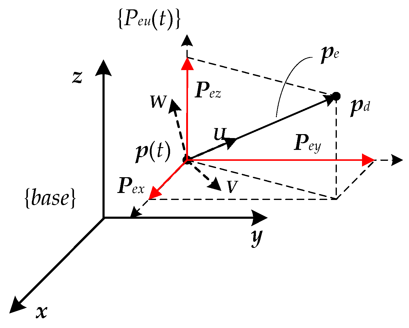
As illustrated in Figure 8, define the current position vector p(t), velocity vector v(t), acceleration vector a(t), and jerk vector j(t), each with n dimensions. Let the target position vector be pd, and the position error vector be pe = pd − p(t). Subsequently, in accordance with the aforementioned principles, obtain the unit orthogonal matrix Peu = [Peu1, Peu2, …, Peun]. {Peu(t)}, or {UVW} coordinate system, is established based on the current pe, representing a local dynamic coordinate system. The corresponding unit orthogonal matrix Peu serves as the projection matrix, allowing the projection of the current pe components relative to the {base} original coordinate system onto the {Peu(t)} system.
At this point, due to the coordinate system projection, the original dimensional directions undergo changes. Consequently, the constraint values must also undergo projection. Define Vimax = min(vmax/Peui), Vimin = min(vmin/Peui), Aimax = min(Amin/Peui), Aimin = min(Amin/Peui), Jimax = min(Jmin/Peui), and Jimin = min(Jmin/Peui), representing the velocity/acceleration/jerk constraints projected onto the new coordinate system. To ensure that the constraints in the new coordinate system do not exceed those in the original coordinate system, the maximum constraint after coordinate system projection is set to the minimum value, and the minimum constraint is set to the maximum value. Subsequently, the current position error, velocity, acceleration, and jerk vectors are projected. Using the dot product, the projected vectors in the coordinate system are obtained as pI(t) = [p1(t), p2(t), …, pn(t)], vI(t) = [v1(t), v2(t), …, vn(t)], aI(t) = [a1(t), a2(t), …, an(t)], jI(t) = [j1(t), j2(t), …, jn(t)].
Subsequently, online planning is conducted, and the updated output control quantity jI(t) is calculated. At this point, our multi-dimensional synchronization algorithm in the projected coordinate system is completed. It is necessary to restore it to the real control coordinate system, and the formula is as follows:
Due to the multi-dimensional nature of joint space planning, synchronous algorithms can also be applied to task space, requiring appropriate transformations for error quantities. Assuming the target state in task space is denoted as pg = [xg, yg, zg, qg], where xg, yg, and zg represent the task space position coordinates and qg denotes the quaternion. For position coordinates, the planning method can be directly applied using Equations (17) and (18). Regarding orientation planning, quaternion calculations are employed to project the orientation error into a three-dimensional space axis-angle representation. The rotation axis is then expanded into a three-dimensional orthogonal coordinate system, and angular velocity is projected onto the new coordinate system for planning angular velocity, angular acceleration, and angular jerk control quantities in each direction. Subsequently, quaternion integration is utilized to compute the quaternion representing the next moment in time. Defining the current unit quaternion as q(t) and the target unit quaternion as qg, the projection of quaternion-represented orientation error onto three-dimensional space is performed, d, and d is expanded into a unit orthogonal matrix Pωu = [Pωu1, Pωu2, …, Pωun], and
where the orientation errors, denoted as pωI(t), ωI(t), aωI(t), and jωI(t) along with angular velocity ω(t), angular acceleration aω(t) and angular jω(t) are calculated to project onto the new orthogonal coordinate system through Equation (19). Drawing an analogy with Equation (18), the positional integration formula can be directly replaced with the quaternion online planning-integration formula for orientation integration:
The algorithm principle involves expanding the unit orthogonal matrix based on position error, where each column represents a new motion direction. By taking the dot product of the position error and velocity with each column, a projection is made in this new direction to obtain the control scalar on this direction. The entire computation process requires only one Schmidt orthogonalization and two matrix projections, thus meeting real-time requirements for efficiency. To emphasize the feasibility of the planning, Table 5 presents the online planning states for only two spaces. In the task space, the orientation information is provided in the form of a unit quaternion.
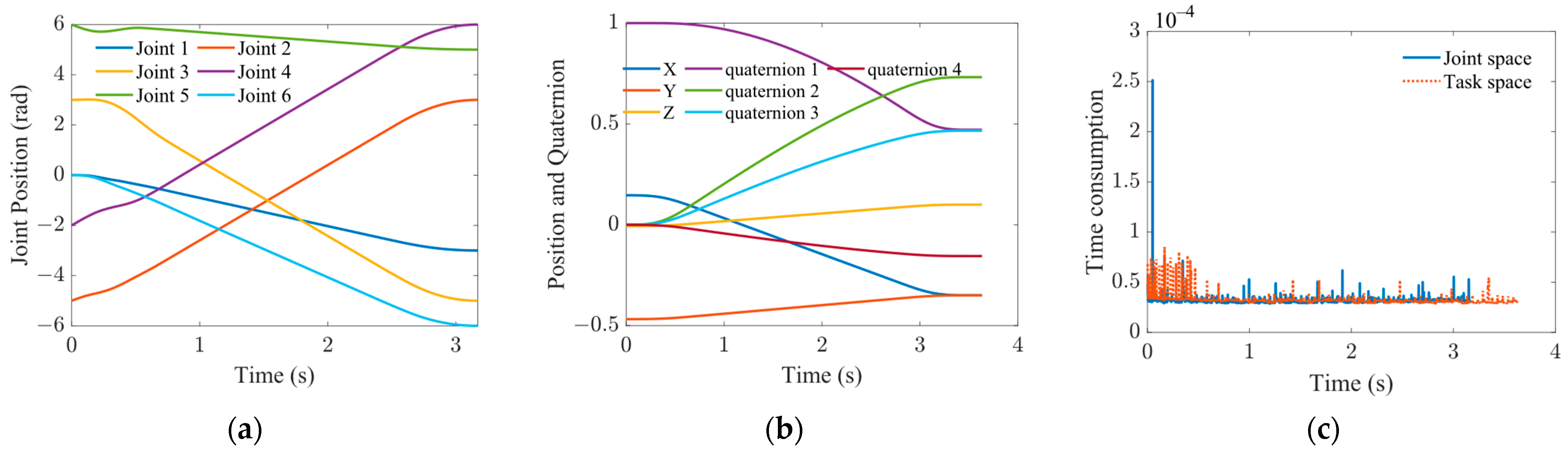
Figure 9 depicts the point-to-point online planning scenarios for both spaces. In Figure 9a, it can be observed that the online planning mode in joint space exhibits slight oscillations compared to the offline mode. This is attributed to the real-time adjustments based on errors, making it highly suitable for applications requiring high dynamic response capabilities. In Figure 9b, the planning in task space appears relatively smooth, maintaining controllability over the end-effector trajectory while retaining high dynamic response capabilities. Figure 9c displays the time consumption for each online trajectory calculation, with each calculation taking less than 1 ms. This demonstrates its feasibility for use in real-time online planning systems.
5. Simulation and Experiment
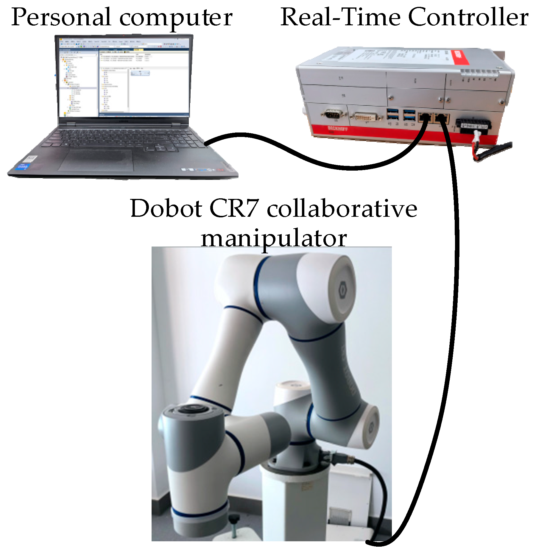
To validate the effectiveness of the algorithm, three verification experiments are conducted in both the task space and joint space. In the task space, the robot performs online velocity planning based on NURBS curves to assess the accuracy of the proposed segmentation method and the effectiveness of the velocity-planning approach. In the joint space, joint online synchronization planning is conducted from arbitrary initial states, validating the practicality of the method through real-time adjustments of joint constraints and target states. Finally, a hybrid space trajectory experiment was conducted to test the robot’s response to unexpected events during task execution. All simulation algorithms were implemented on a personal computer equipped with an Intel Core i7-11800H CPU (2.30 GHz) and 64 GB RAM, using MATLAB R2022b (The MathWorks, Natick, MA, USA). As shown in Figure 10, the experimental setup featured a Dobot CR7 collaborative manipulator [38], controlled by a Beckhoff C6930-0060 controller [39]. The controller was equipped with an Intel Core i7-6700TE 2.4 GHz CPU and 8 GB of memory. Communication between the controller and the robot motor drives occurred via the EtherCAT protocol at a sampling rate of 500 Hz, resulting in a sampling period of 2 ms.
5.1. Online Trajectory Generation Testing in the Task Space
Simulated experiments were conducted in this section to confirm the effectiveness of the NURBS curve discretization approach proposed in this paper, which is based on chord error constraint. The effectiveness of online feed-rate scheduling and segmented spline interpolation was also evaluated. The butterfly curve was chosen as a widely-used example, and its parameters, along with those for the trajectory planning, are presented in Table 6. The standard butterfly NURBS curve was discretized and segmented into 193 Bezier curves. Maximum feed rate Vmax was set as 10 mm/s and dynamic feed rate adjustments were implemented in different motion segments.
Figure 11a illustrates the chord error of each curve, while Figure 11b illustrates the corresponding curvatures. The results confirm that the proposed curve discretization method effectively controls the chord error of the curves within the constraint.
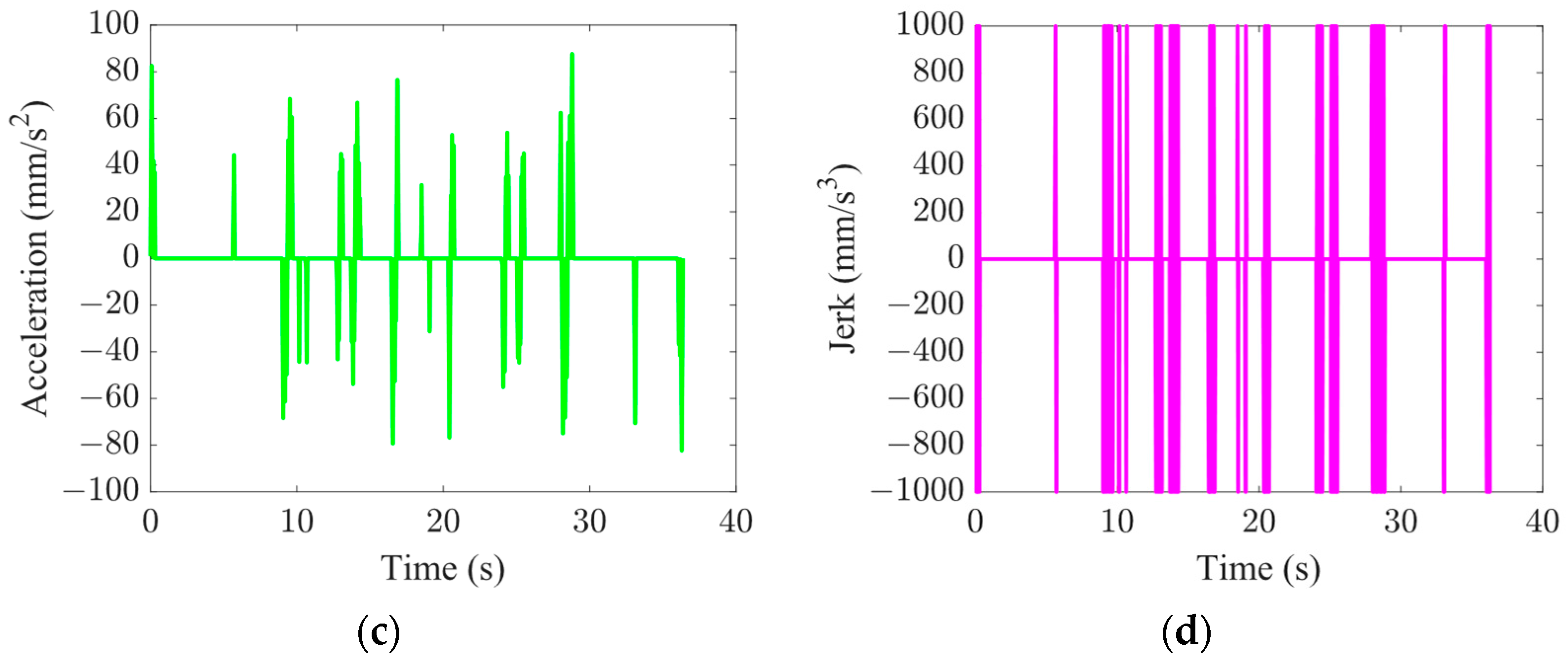
Figure 12 displays the displacement and feed-rate profiles of the butterfly NURBS curve, which are based on online S-shape feed-rate scheduling. The bidirectional scanning constrains [34] the feed rate of 193 Bezier curves. For feed-rate scheduling and interpolation, the accurate arc length of the curve must first be calculated. Employing the composite Simpson’s rule [35] for evaluating the arc length can be viewed as a continuous iterative procedure for determining the value of the parameter u. Figure 12a displays the segmented results of the butterfly curve, where curves of different colors represent Bezier curves satisfying the chord error. The results of dynamic feed-rate adjustments are illustrated in Figure 12b. It can be observed that the actual feed rate is dynamically adjusted according to different maximum feed rates, validating the effectiveness of the feed rate adjustment measures proposed in this study. Figure 12c illustrates the acceleration profile, indicating that the acceleration throughout the process strictly adheres to the specified acceleration constraint parameters. Figure 12d provides the jerk profile, which is strictly planned according to the given values. This validates the effectiveness of the feed-rate adjustment measures and parameter constraints proposed in this study.
5.2. Online Trajectory-Generation Testing in the Joint Space
The initial state parameters of the joints and dynamic position parameters are provided in Table 7, and the trajectory is illustrated in Figure 13.
Due to the utilization of the real-time projection matrix synchronization algorithm, the algorithm supports the modification of the target position at any given moment. At 0.5 s, modifications to the target positions of joints 1, 3, and 5 were performed online; At 1 s, joints 2, 4, and 6 underwent online modifications to their target positions; at 2 s, modifications to the online target positions were applied to all joints. The entire process enables synchronous planning for multiple joints, highlighting the versatility of the projection matrix synchronization method, which establishes a multidimensional orthogonal projection matrix based on the current state. When certain joints or dimensions are modified, it synchronously influences the entire projection space, re-establishing mapping relationships to achieve synchronization in other dimensions that have not undergone modification of the target state. Figure 13 illustrates the corresponding joint position, velocity, and acceleration profiles. It can be verified that the planning results conform to the constraints of the specified parameters. As mentioned earlier, the online synchronization algorithm based on the error projection matrix possesses highly dynamic response capabilities. However, their drawback lies in the inability to reduce the acceleration to zero at the endpoint, although velocity can be reduced to zero. Therefore, this planning method is highly suitable for scenarios where unexpected events trigger such planning modes. Furthermore, it also validates that the real-time error projection matrix synchronization method proposed in this paper can achieve synchronization, satisfying multi-dimensional constraints.
5.3. The Trajectory Testing in Hybrid Space
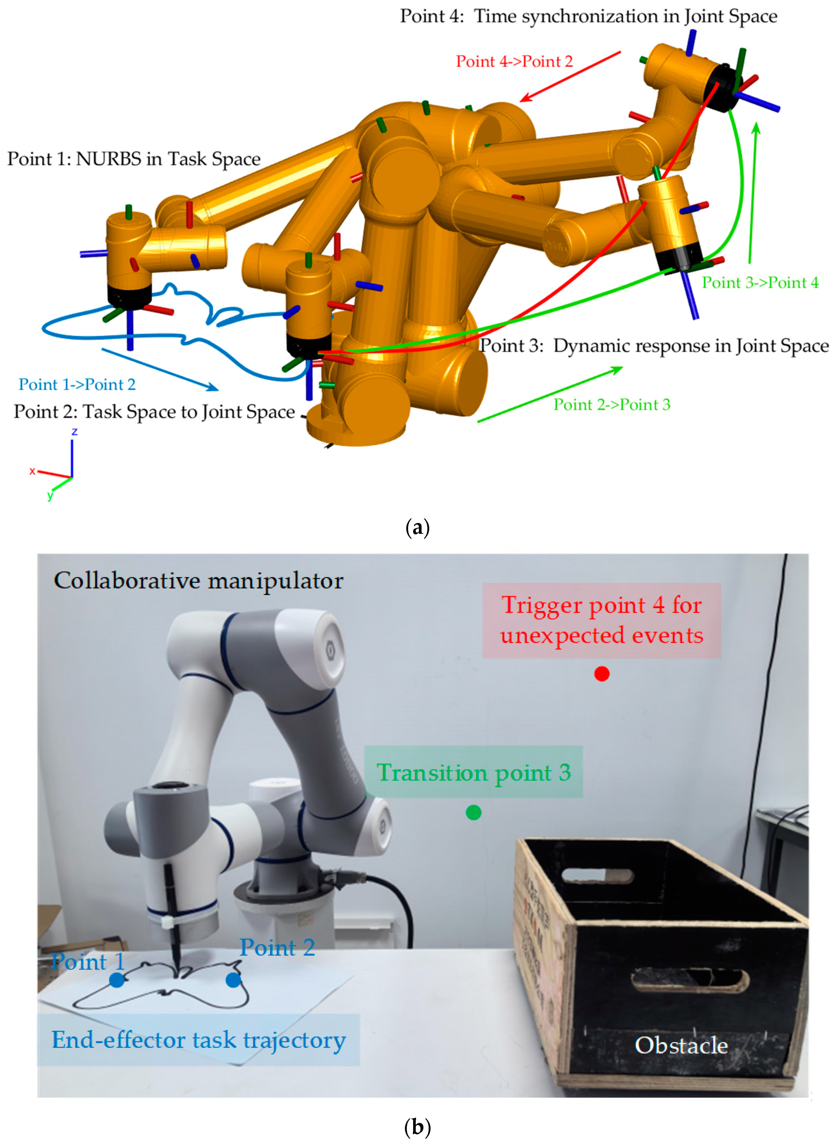
Testing the manipulator’s response to unexpected events during task execution involves guiding the task space trajectory between control points 1 and 2, ensuring precise task completion at the end-effector. An unexpected event is triggered at control point 2, such as tool damage requiring immediate replacement. The system transitions to control point 4, considering potential collisions with the surrounding environment, necessitating the introduction of control point 3 for a smooth transition. After the end-effector tool replacement is complete, control point 4 utilizes a joint synchronous motion to seamlessly continue the remaining task planning from control point 2. This experiment serves to test the entire logic of the hybrid space online trajectory control, validating the effectiveness of the proposed approach. The complete simulation is depicted in Figure 14a, while Figure 14b illustrates the actual manipulator workspace.
Table 8 provides the joint space position information for four points. Since triggering unexpected events from the task space to the joint space requires Jacobian transformation, joint space positions can be solved using inverse kinematics. The constraint parameters for joint space planning are set according to Table 7.
In practical application scenarios, singular paths often exist in task space, and they can be avoided by planning ahead to prevent singular points in the path. If in an unknown environment, the real-time prediction and trajectory-generation processing of singular points is a future research problem worth exploring. According to the proposed solution in this paper, one possible approach could involve handling singular points through joint space transitions. When the robotic arm enters a singular region, future Cartesian path points can be obtained through foresight. By solving inverse kinematics, stable joint angles can be obtained. Combined with the Jacobian matrix and foresight velocity, corresponding joint velocities can be obtained. The decision on the planning method can be made based on real-time requirements. For scenarios with high accuracy requirements and long foresight distances, offline joint synchronization may be adopted. For scenarios with high response speed requirements and short foresight distances, online joint synchronization may be more suitable. This will be a direction for future research.
6. Conclusions
The algorithm still has certain limitations, which restrict its application scenarios. Therefore, selecting algorithms with different performance characteristics for different scenarios is also the endpoint that this paper aims to illustrate. For example, online planning in Cartesian space can perform dynamic speed adjustments. Since it is designed for the incremental planning of spatial displacement, it can obtain displacement for a given path to ensure trajectory accuracy. However, this makes the algorithm incompatible with situations involving both positive and negative motions, such as those in joint space. Offline synchronization in joint space ensures high flexibility and smoothness but is not suitable for scenarios requiring a highly dynamic response due to the lengthy iterative calculations and judgments involved. Online synchronization in both joint and task space aims to address highly dynamic response issues by performing real-time planning based on current states, resulting in high computational efficiency and strong constraints. It adapts well to dynamic target planning in unknown environments. However, joint synchronization may lead to slight oscillations, while task space synchronization forms linear trajectories and cannot be applied to curved trajectories.
This paper proposes a trajectory-generation method tailored for serial robots in hybrid space operations. In task space operations, this paper introduces a NURBS discretization calculation method that relies on the convex hull property of spline curves. Incorporating chord error constraints ensures the contour accuracy of the trajectory in the task space. The combination of spatial curve displacement and an online feed-rate scheduling method ensures end-effector stability, making it suitable for high-precision tasks. In the joint space, an offline mode time-synchronized planning algorithm is initially proposed to ensure smooth joint motion. To address unexpected events, a dynamic multi-joint synchronization algorithm is devised based on an error-projection matrix. This algorithm effectively integrates global feedback and local dynamic projection to ensure the effectiveness of synchronizing various joint motions, yielding favorable results in the execution of motion on serial robot systems. The results of simulations and experiments confirm the effectiveness of this approach.
Author Contributions
Y.X. contributed the central idea and wrote the initial draft of the paper. Y.L., X.L., Y.Z., P.L. and P.X. contributed to the refining of the ideas and revised this paper. Software and writing—original draft, Y.X.; Resources and writing—original draft, Y.L. and X.L.; Writing—review and editing, Y.Z., P.L. and P.X. All authors have read and agreed to the published version of the manuscript.
Funding
This work was supported by the Fundamental Research Funds for the Central Universities, Grant No. 2572023CT15-03.
Data Availability Statement
All data generated or analyzed during this study are included in this paper or are available from the corresponding authors on reasonable request.
Conflicts of Interest
The authors declare no conflicts of interest.
References
- Gasparetto, A.; Boscariol, P.; Lanzutti, A.; Vidoni, R. Motion and Operation Planning of Robotic Systems; Springer: Cham, Switzerland, 2015; pp. 3–27. [Google Scholar]
- Bianco, C.G.L.; Faroni, M.; Beschi, M.; Visioli, A. A predictive technique for the real-time trajectory scaling under high-order constraints. IEEE/ASME Trans. Mechatron. 2021, 27, 315–326. [Google Scholar] [CrossRef]
- Haschke, R.; Weitnauer, E.; Ritter, H. On-line planning of time-optimal, jerk-limited trajectories. In Proceedings of the 2008 IEEE/RSJ International Conference on Intelligent Robots and Systems, Nice, France, 22–26 September 2008; pp. 3248–3253. [Google Scholar]
- Huang, L.; Feng, D.; Huang, D.; Dong, X.; Huang, D. Research on Trajectory Planning for multiple straight lines in Cartesian Space. In Proceedings of the 2023 IEEE International Conference on Mechatronics and Automation (ICMA), Harbin, China, 6–9 August 2023; pp. 942–947. [Google Scholar]
- Gao, M.; Chen, D.; Din, P.; He, Z.; Wu, Z.; Liu, Y. A fixed-distance Cartesian path planning algorithm for 6-DOF industrial robots. In Proceedings of the 2015 IEEE 24th International Symposium on Industrial Electronics (ISIE), Buzios, Brazil, 3–5 June 2015; pp. 616–620. [Google Scholar]
- Kröger, T.; Wahl, F.M. Online trajectory generation: Basic concepts for instantaneous reactions to unforeseen events. IEEE Trans. Robot. 2009, 26, 94–111. [Google Scholar] [CrossRef]
- Piazzi, A.; Visioli, A. Global minimum-jerk trajectory planning of robot manipulators. IEEE Trans. Ind. Electron. 2000, 47, 140–149. [Google Scholar] [CrossRef]
- Bianco, C.G.L. An efficient algorithm for the real-time generation of synchronous reference signals. IEEE Trans. Ind. Electron. 2016, 64, 4621–4630. [Google Scholar] [CrossRef]
- Tagliavini, A.; Bianco, C.G.L. A Smooth Orientation Planner for Trajectories in the Cartesian Space. IEEE Robot. Autom. Lett. 2023, 8, 2606–2613. [Google Scholar] [CrossRef]
- Tagliavini, A.; Bianco, C.G.L. η3D-splines for the generation of 3D Cartesian paths with third order geometric continuity. Robot. Comput. Integr. Manuf. 2021, 72, 102203. [Google Scholar] [CrossRef]
- Lavernhe, S.; Tournier, C.; Lartigue, C. Optimization of 5-axis high-speed machining using a surface based approach. Comput. Aided Des. 2008, 40, 1015–1023. [Google Scholar] [CrossRef]
- Sarkar, S.; Dey, P.P. A new iso-parametric machining algorithm for free-form surface. Proc. IMechE Part E J. Eng. Manuf. 2014, 228, 197–209. [Google Scholar] [CrossRef]
- Li, H.; Zhang, L. Geometric error control in the parabola-blending linear interpolator. J. Syst. Sci. Complex. 2013, 26, 777–798. [Google Scholar] [CrossRef]
- Lee, R.S.; She, C.H. Tool path generation and error control method for multi-axis NC machining of spatial cam. International Int. J. Mach. Tools Manuf. 1998, 38, 277–290. [Google Scholar] [CrossRef]
- Huang, J.; Zhu, L.M. Feedrate scheduling for interpolation of parametric tool path using the sine series representation of jerk profile. Proc. Inst. Mech. Eng. Part E J. Eng. Manuf. 2017, 231, 2359–2371. [Google Scholar] [CrossRef]
- Lin, M.T.; Tsai, M.S.; Yau, H.T. Development of a dynamics-based NURBS interpolator with real-time look-ahead algorithm. Int. J. Mach. Tools Manuf. 2007, 47, 2246–2262. [Google Scholar] [CrossRef]
- Liang, F.; Yan, G.; Fang, F. Global time-optimal B-spline feedrate scheduling for a two-turret multi-axis NC machine tool based on optimization with genetic algorithm. Robot. Comput. Integr. Manuf. 2022, 75, 102308. [Google Scholar] [CrossRef]
- Ni, H.; Zhang, C.; Ji, S.; Hu, T.; Chen, Q.; Liu, Y.; Wang, G. A bidirectional adaptive feedrate scheduling method of NURBS interpolation based on S-shaped ACC/DEC algorithm. IEEE Access 2018, 6, 63794–63812. [Google Scholar] [CrossRef]
- Fan, W.; Gao, X.S.; Yan, W.; Yuan, C.M. Interpolation of parametric CNC machining path under confined jounce. Int. J. Adv. Manuf. Technol. 2012, 62, 719–739. [Google Scholar] [CrossRef]
- Song, F.; Yu, S.; Chen, T.; Sun, L.N. Research on CNC simulation system with instruction interpretations possessed of wireless communication. J. Supercomput. 2016, 72, 2703–2719. [Google Scholar] [CrossRef]
- Li, H.; Le, M.D.; Gong, Z.M.; Lin, W. Motion profile design to reduce residual vibration of high-speed positioning stages. IEEE/ASME Trans. Mechatron. 2009, 14, 264–269. [Google Scholar]
- Bai, Y.; Chen, X.; Yang, Z. A Generic Method to Generate AS-Curve Profile in Commercial Motion Controller. In Proceedings of the ASME 2017 International Design Engineering Technical Conferences and Computers and Information in Engineering Conference, Cleveland, OH, USA, 6–9 August 2017; p. V009T07A047. [Google Scholar]
- He, S.; Hu, C.; Lin, S.; Zhu, Y. An online time-optimal trajectory planning method for constrained multi-axis trajectory with guaranteed feasibility. IEEE Robot. Autom. Lett. 2022, 7, 7375–7382. [Google Scholar] [CrossRef]
- Verscheure, D.; Demeulenaere, B.; Swevers, J.; De Schutter, J.; Diehl, M. Time-optimal path tracking for robots: A convex optimization approach. IEEE Trans. Autom. Control 2009, 54, 2318–2327. [Google Scholar] [CrossRef]
- Nagy, A.; Vajk, I. Sequential time-optimal path-tracking algorithm for robots. IEEE Trans. Robot. 2019, 35, 1253–1259. [Google Scholar] [CrossRef]
- Faroni, M.; Beschi, M.; Bianco, C.G.L.; Visioli, A. Predictive joint trajectory scaling for manipulators with kinodynamic constraints. Control Eng. Pract. 2020, 95, 104264. [Google Scholar] [CrossRef]
- Pham, Q.C. A general, fast, and robust implementation of the time-optimal path parameterization algorithm. IEEE Trans. Robot. 2014, 30, 1533–1540. [Google Scholar] [CrossRef]
- Pham, H.; Pham, Q.C. A new approach to time-optimal path parameterization based on reachability analysis. IEEE Trans. Robot. 2018, 34, 645–659. [Google Scholar] [CrossRef]
- Lindner, T.; Milecki, A. Reinforcement Learning-Based Algorithm to Avoid Obstacles by the Anthropomorphic Robotic Arm. Appl. Sci. 2022, 12, 6629. [Google Scholar] [CrossRef]
- Kim, M.; Han, D.K.; Park, J.H.; Kim, J.S. Motion Planning of Robot Manipulators for a Smoother Path Using a Twin Delayed Deep Deterministic Policy Gradient with Hindsight Experience Replay. Appl. Sci. 2020, 10, 575. [Google Scholar] [CrossRef]
- Bianco, C.G.L.; Raineri, M. An experimentally validated technique for the real-time management of wrist singularities in nonredundant anthropomorphic manipulators. IEEE Trans. Control Syst. Technol. 2019, 28, 1611–1620. [Google Scholar] [CrossRef]
- Berscheid, L.; Kröger, T. Jerk-limited real-time trajectory generation with arbitrary target states. Robot. Sci. Syst. XVII 2021. [Google Scholar] [CrossRef]
- Boehm, W. Inserting new knots into B-spline curves. Comput. Aided Des. 1980, 12, 199–201. [Google Scholar] [CrossRef]
- Du, X.; Huang, J.; Zhu, L.M. A complete S-shape feed rate scheduling approach for NURBS interpolator. J. Comput. Des. Eng. 2015, 2, 206–217. [Google Scholar] [CrossRef]
- Lei, W.T.; Sung, M.P.; Lin, L.Y.; Huang, J.J. Fast real-time NURBS path interpolation for CNC machine tools. Int. J. Mach. Tools Manuf. 2007, 47, 1530–1541. [Google Scholar] [CrossRef]
- Biagiotti, L.; Melchiorri, C. Trajectory Planning for Automatic Machines and Robots; Springer: Berlin/Heidelberg, Germany, 2008. [Google Scholar]
- Gerelli, O.; Bianco, C.G.L. A discrete-time filter for the on-line generation of trajectories with bounded velocity, acceleration, and jerk. In Proceedings of the 2010 IEEE International Conference on Robotics and Automation, Anchorage, AK, USA, 3–7 May 2010; pp. 3989–3994. [Google Scholar]
- CR7 Collaborative Robot. Available online: https://www.dobot-robots.com/products/cr-series/cr7.html (accessed on 27 April 2023).
- C6930-0060|Control Cabinet Industrial PC. Available online: https://www.beckhoff.com/en-us/products/ipc/pcs/c69xx-compact-industrial-pcs/c6930-0060.html (accessed on 2 November 2022).
Figure 1.
The segmentation algorithm. (a) A NUBRS curve; (b) segment NUBRS curve to four Bezier curves. The curves are shown as different colors; (c) the distance between control points and the local frame of Bezier1; (d) under the condition of satisfying the chord error constraint, segment Bezier 1 to 15 Bezier curves.

Figure 2.
Under the condition of satisfying the chord error constraint: (a) the original NURBS curve is divided into 47 Bezier segments. (b) Different curves segmentation results.
Figure 2.
Under the condition of satisfying the chord error constraint: (a) the original NURBS curve is divided into 47 Bezier segments. (b) Different curves segmentation results.

Figure 3.
Illustration of the first segment and the second segment.

Figure 4.
The algorithm flow of online feed-rate scheduling based on spatial displacement.

Figure 5.
Simulation result of online S-shape feed rate scheduling with dynamic constraints: (a) displacement; (b) feed rate; (c) acceleration; (d) jerk.
Figure 5.
Simulation result of online S-shape feed rate scheduling with dynamic constraints: (a) displacement; (b) feed rate; (c) acceleration; (d) jerk.

Figure 6.
The algorithm flow of velocity planning based on time-constrained mode.

Figure 7.
The simulation of joint feed-rate scheduling: (a) without time synchronization; (b) with maximum time synchronization.
Figure 7.
The simulation of joint feed-rate scheduling: (a) without time synchronization; (b) with maximum time synchronization.

Figure 8.
The projection matrix.

Figure 9.
The simulation of online synchronization algorithm: (a) joint space; (b) task space; (c) the time consumption for each calculation.
Figure 9.
The simulation of online synchronization algorithm: (a) joint space; (b) task space; (c) the time consumption for each calculation.

Figure 10.
The experiment platform.

Figure 11.
Simulation. (a) The chord error; (b) the curvature.

Figure 12.
Simulation for butterfly curve: (a) butterfly NUBRS; (b) feed rate of online S-shape feed-rate scheduling; (c) acceleration profile; (d) jerk profile.
Figure 12.
Simulation for butterfly curve: (a) butterfly NUBRS; (b) feed rate of online S-shape feed-rate scheduling; (c) acceleration profile; (d) jerk profile.


Figure 13.
Simulation for online joint synchronization planning.

Figure 14.
The result of simulation and physical experiment: (a) simulation; (b) physical experiment.
Figure 14.
The result of simulation and physical experiment: (a) simulation; (b) physical experiment.


Table 1.
Bezier parameters obtained with node insertion technique in Figure 1b.
Table 1.
Bezier parameters obtained with node insertion technique in Figure 1b.
| Curve Types | Node Vectors | |
|---|---|---|
| NUBRS | ||
| Bezier 1 | ||
| Bezier 2 | ||
| Bezier 3 | ||
| Bezier 4 |
Table 2.
Performance parameters table for different methods.
| Parameters | M.L. [16] | X.D. [34] | W.L. [35] | Ours |
|---|---|---|---|---|
| Number of iterations | \ | \ | \ | 3 |
| Iterations computational time (s) | \ | \ | \ | 0.001 |
| Max chord error (mm) | 1.5 | 1.5 | 1.2 | 0.1 |
| End value of u | 0.997 | 0.997 | 0.997 | 1 |
| Truncation error (mm) | 0.001 | 0.001 | 0.001 | 0 |
Table 3.
The parameter of online feed-rate scheduling.
| Time(s) | Vmax (mm/s) | Vmin (mm/s) | Amax (mm/s2) | Amin (mm/s2) | Jmax (mm/s3) | Jmin (mm/s3) |
|---|---|---|---|---|---|---|
| 5 | −6 | 10 | −12 | 20 | −25 | |
| 15 | −13 | 12 | −15 | 90 | −100 | |
| t ≥ 6 | 30 | −50 | 30 | −20 | 70 | −80 |
Table 4.
The parameter of feed rate scheduling.
| Parameters | Joint 1 | Joint 2 | Joint 3 | Joint 4 | Joint 5 | Joint 6 |
|---|---|---|---|---|---|---|
| vs (rad/s) | 0 | −4 | 3 | −2 | 0 | 3 |
| ve (rad/s) | 0 | 6 | 7 | −5 | −6 | −8 |
| as (rad/s2) | 0 | 1 | −2 | 3 | 5 | −2 |
| ae (rad/s2) | 0 | 2 | −3 | −1 | 4 | 0 |
| Initial joint position (rad) | 0 | −2 | 3 | −4 | 5 | 1 |
| Target joint position (rad) | 4 | −6 | 10 | 2 | 0 | −5 |
| Execution time (s) | 0.6000 | 0.6519 | 0.7756 | 0.9145 | 0.6290 | 0.7559 |
| Constraint | Vmax (rad/s) | Vmin (rad/s) | Amax (rad/s2) | Amin (rad/s2) | Jmax (rad/s3) | Jmin (rad/s3) |
| Value | 10 | −10 | 100 | −100 | 1000 | −1000 |
Table 5.
The online planning states for two spaces.
| Initial Position | Target Position | |
|---|---|---|
| Joint Space (rad) | [0,−5,3,−2,6,0] | [−3,3,−5,6,5,−6] |
| Task Space (xyz quaternion: 1–4) | [0.1463,−0.4679,−0.0066] [1,0,0,0] | [−0.35,−0.35,0.1] [0.4711,0.7322,0.4668,−0.1551] |
Table 6.
Test parameters of the interpolations.
| Parameters | Symbols (unit) | Values |
|---|---|---|
| Chord error tolerance | δ (mm) | 0.05 |
| Interpolator period | ts (s) | 0.001 |
| Maximum tangential acceleration | Atmax (mm/s2) | 100 |
| Minimum tangential acceleration | Atmin (mm/s2) | −100 |
| Maximum normal acceleration | Anmax (mm/s2) | 120 |
| Minimum normal acceleration | Anmin (mm/s2) | −120 |
| Max jerk | Jmax (mm/s3) | 1000 |
| Min jerk | Jmin (mm/s3) | −1000 |
| Maximum feed rate | Vmax (mm/s) | 10 |
| 12 (20–45 segments) | ||
| 8 (50–60 segments) | ||
| 14 (70–85 segments) | ||
| 11 (95–100 segments) | ||
| 15 (150–180 segments) |
Table 7.
The dynamic position of the joints.
| Parameters | Target Position (rad) | Initial Position (rad) | Initial Velocity (rad/s) | Initial Acceleration (rad/s2) | Velocity Constraint (rad/s) | Acceleration Constraint (rad/s2) | |
|---|---|---|---|---|---|---|---|
| Time (s) | |||||||
| [−3,3,−5,6,6,−6] | |||||||
| [6,3,2,6,−10,−6] | |||||||
| [6,−5,2,20,−10,−1] | |||||||
| [5,10,−5,3,−6,0] | |||||||
Table 8.
The position of the points.
| Position (rad) | |
|---|---|
| Point 1 | [−2.4784, −1.6947,2.0595, −1.9373, −1.5708, −0.9146] |
| Point 2 | [−1.5427, −1.6954,2.0565, −1.9319, −1.5708,0.0281] |
| Point 3 | [−0.4119, −1.0036,0.8622, −1.8675, −1.5708,0.0281] |
| Point 4 | [0.0281, −1.1292,0.8622, −2.6878, −1.5708,0.0281] |
Disclaimer/Publisher’s Note: The statements, opinions and data contained in all publications are solely those of the individual author(s) and contributor(s) and not of MDPI and/or the editor(s). MDPI and/or the editor(s) disclaim responsibility for any injury to people or property resulting from any ideas, methods, instructions or products referred to in the content. |
© 2024 by the authors. Licensee MDPI, Basel, Switzerland. This article is an open access article distributed under the terms and conditions of the Creative Commons Attribution (CC BY) license (https://creativecommons.org/licenses/by/4.0/).
Share and Cite
MDPI and ACS Style
Xu, Y.; Liu, Y.; Liu, X.; Zhao, Y.; Li, P.; Xu, P. Trajectory Generation Method for Serial Robots in Hybrid Space Operations. Actuators 2024, 13, 108. https://0-doi-org.brum.beds.ac.uk/10.3390/act13030108
AMA Style
Xu Y, Liu Y, Liu X, Zhao Y, Li P, Xu P. Trajectory Generation Method for Serial Robots in Hybrid Space Operations. Actuators. 2024; 13(3):108. https://0-doi-org.brum.beds.ac.uk/10.3390/act13030108
Chicago/Turabian StyleXu, Yan, Yaqiu Liu, Xun Liu, Yiyang Zhao, Peibo Li, and Pengjie Xu. 2024. "Trajectory Generation Method for Serial Robots in Hybrid Space Operations" Actuators 13, no. 3: 108. https://0-doi-org.brum.beds.ac.uk/10.3390/act13030108
Note that from the first issue of 2016, this journal uses article numbers instead of page numbers. See further details here.