
Trajectory Re-Planning and Tracking Control for a Tractor–Trailer Mobile Robot Subject to Multiple Constraints

1
School of Mechanical Engineering, Shanghai Jiao Tong University, Shanghai 200240, China
2
College of Mechanical Engineering, Donghua University, Shanghai 200051, China
3
Zhejiang Lab, Hangzhou 311121, China
*
Author to whom correspondence should be addressed.
Actuators 2024, 13(3), 109; https://0-doi-org.brum.beds.ac.uk/10.3390/act13030109
Submission received: 31 January 2024
/
Revised: 4 March 2024
/
Accepted: 6 March 2024
/
Published: 8 March 2024
(This article belongs to the Special Issue Advances in Dynamics and Motion Control of Unmanned Aerial/Underwater/Ground Vehicles)
Abstract
:Autonomous tractor–trailer robots possess a broad spectrum of applications but pose significant challenges in control due to their nonlinear and underactuated dynamics. Unlike the tractor, the motion of the trailer cannot be directly actuated, which often results in a deviation from the intended path. In this study, we introduce a novel method for generating and following trajectories that circumvent obstacles, tailored for a tractor–trailer robotic system constrained by multiple factors. Firstly, leveraging the state information of both the obstacles and the desired trajectory, we formulate an improved trajectory for obstacle avoidance using the nonlinear least squares method. Subsequently, we propose an innovative tracking controller that integrates a universal barrier function with a state transformation strategy. This amalgamation facilitates the accurate tracking of the prescribed trajectory. Our theoretical analysis substantiates that the proposed control methodology ensures exponential convergence of the line-of-sight (LOS) distance and angle tracking errors, while enhancing the transient performance. To validate the efficacy of our approach, we present a series of simulation results, which demonstrate the applicability of the developed control strategy in managing the complex dynamics of tractor–trailer robots.
1. Introduction
The Tractor–Trailer Wheeled-Robot (TTWR) system, with its intrinsic capability to tow trailers and transport payloads, holds considerable potential for a myriad of practical applications spanning the domains of agriculture, transportation, and beyond [1,2,3,4,5,6,7]. Nevertheless, the inherently nonlinear and underactuated dynamics of the TTWR system present intricate challenges in terms of its planning and control faculties. Moreover, as a multi-body entity, the TTWR system is susceptible to complications such as self-collision and the potential for structural folding [8,9,10], further exacerbating the complexity of research endeavors in this field.
Despite these challenges, advancements in system identification technologies coupled with the progression of nonlinear control theory have significantly deepened the understanding and refinement of planning and control strategies for the TTWR system. The research dedicated to TTWR systems encompasses a diverse array of focal areas, including the formulation of kinematic and dynamic models, stability analysis, stabilization control methodologies, and the precision of trajectory tracking control mechanisms [11,12,13,14,15,16,17,18,19]. These research streams are critical for unlocking the full potential of TTWR systems and facilitating their integration into the targeted fields of application.
TTWRs are stratified into various classifications based on their maneuverability and controllability, with two predominant kinematic models garnering substantial scholarly interest. The first model pertains to a differential steering configuration, wherein two differentially driven wheels are employed as the primary means of propulsion. The alternative model incorporates an Ackermann steering mechanism, which utilizes the tractor’s front wheels for directional guidance and the rear wheels for propelling and towing the trailer. Kinematic models of these two types are studied in [20]. In our research, we focus on the first type, i.e., differential wheel steering.
In the field of control theory, the overarching goal of system motion control is to manage and direct the behavior of dynamic systems, and this is typically bifurcated into two fundamental categories: stabilization control [14,15,21,22] and tracking control [23,24,25,26,27,28,29].
Stabilization control focuses on the system’s ability to attain and maintain a state of equilibrium. The objective is to design control laws that ensure the states of system converge to the equilibrium points, despite any disturbances or inherent system fluctuations. This type of control is vital for systems where maintaining a steady state is essential for operational stability and safety.
On the other hand, tracking control is concerned with the system’s capability to follow a predefined trajectory over time. This trajectory represents the desired path or set of states that the system should achieve throughout its operation. Tracking control is crucial in applications where the system must follow a particular route or pattern, such as in autonomous vehicles, robotic manipulators, and other automated systems where precise motion is required. In this paper, our research focuses on the tracking control.
The complexity of the tracking control task is compounded by a variety of constraints, which must be accounted for to ensure the system’s safety and performance. Among these constraints, heading angle limitations, LOS distance restrictions, and obstacle avoidance are prevalent.
In reference [30], the authors introduce a generic obstacle avoidance function, meticulously engineered to ensure that the LOS distance and angle errors converge within prescribed limits. This method underscores the importance of designing control strategies that are compliant with constraints while achieving the intended control objectives. Furthermore, for dealing with uncertainty and external disturbances, an adaptive control framework was integrated into this method [31]. It enhanced the robustness of system. This adaptation is crucial in practical applications where perfect knowledge of the environment is unattainable. Reference [32] expended this approach into the tracking control of multi-robot systems, enabling them to collectively track desired trajectories while adhering to a set of constraints. Such collective coordination is imperative in scenarios where multiple robots operate in a shared space or where formation control is required.
In the context of robotic control, the obstacle avoidance constraint cannot be ignored. However, within the control issues of TTWR, research on obstacle avoidance has seldom been the focus of attention. This paper makes a preliminary exploration into the control problem of TTWRs with obstacle avoidance constraints, which is accomplished based on the assumptions of low-speed operation and precise tracking.
In the pertaining literature, two efficacious methods for trajectory tracking control of TTWR were proposed in [13,31]. The methodology espoused in [13] employs the backstepping technique, commencing with the conversion of the original system into an error system via state and input transformations. A virtual controller is then meticulously crafted to ensure the closed-loop system’s stability. Despite its effectiveness, this approach is criticized for its complexity and lack of intuitive clarity, particularly as the methodology for translating the virtual input vector into a tangible input vector remains unaddressed. Conversely, reference [31] advances the discourse by introducing a barrier Lyapunov function predicated on distance error and devises a control law that not only complies with the LOS distance constraints but also boasts a more streamlined structural composition. Nonetheless, this method is not without its limitations, as it exhibits suboptimal transient responses within the closed-loop system.
The present paper endeavors to surmount the limitations inherent in these aforementioned strategies by proposing a novel LOS control law. This newly formulated law is characterized by its structural simplicity, obviating the need for input transformations, and simultaneously enhances the transient performance of the closed-loop system. Furthermore, this study introduces a trajectory re-planning scheme predicated on nonlinear least squares. This scheme is adept at navigating around static obstacles, thereby augmenting the TTWR system’s operational robustness and adaptability to complex environments.
The structure of the remainder of this paper is as follows: Section 2 details the materials and methodologies utilized. This includes a system overview and the necessary background knowledge, presented in Section 2.1 and Section 2.2, respectively. Section 2.3 introduces trajectory re-planning using the nonlinear least squares technique. Section 2.4 then describes the development of a novel control law for the TTWR system, predicated upon the tractor’s LOS distance and angle, which are informed by the re-planned trajectory. Section 3 is devoted to the presentation of experimental results. Within this section, Section 3.1 and Section 3.2 examine scenarios with and without the presence of obstacles, respectively, to validate the effectiveness of the proposed approach. Section 4 concludes the paper with a summary and discussion of the findings.
2. Materials and Methods
2.1. System Description
Consider the tractor–trailer mobile robot depicted in Figure 1, wherein the tractor is outfitted with two driven wheels, and the trailer is mounted on two passive wheels. Given the assumption of planar motion and the premise that the vehicle’s wheels, modeled as thin solid disks, are non-slipping in the lateral direction, the kinematic equations governing the tractor–trailer mobile robot system can be expressed as delineated in [30,31]:
Figure 1 illustrates the configuration of a tractor–trailer system, where the midpoint of the tractor’s wheels is represented by point , possessing coordinates in the inertial reference frame. Correspondingly, the midpoint of the trailer’s wheels is indicated by point , with coordinates also in the inertial reference frame. The heading angles of the tractor and trailer are denoted by and , respectively, and are measured relative to the inertial frame. A rigid linkage of length connects point on the tractor to point on the trailer, thereby establishing the kinematic relationship between the two components. The control inputs for the system are twofold: the linear velocity at point on the tractor and the angular velocity associated with the tractor’s heading angle .
Remark 1.
Taking into account the practical constraints of the system, actuation is achieved through manipulation of the driven wheel angles. Let and represent the angular positions of the left and right tractor wheels, respectively. The control inputs, namely the linear velocity and the angular velocity , can be derived from these wheel angles as follows:
where the symbol r denotes the radius of the tractor’s wheel, whereas b signifies the half-width of the vehicle, corresponding to the lateral distance between the centers of the two driving wheels.
Remark 2.
When a trailer is tasked with tracking a predetermined trajectory, it is imperative to ascertain the necessary positional and velocity parameters of the trailer. The velocity data are instrumental in defining the requisite heading angle of the trailer. Utilizing this data, the anticipated position and velocity of the tractor can be extrapolated from the desired trajectory of the trailer. In accordance with the kinematic model governing the tractor–trailer system, it can be established that a specific relational expression binds the motion of the tractor to that of the trailer:
Within the equation, Equation (3) is self-evident, thus its explanation is omitted. The proof for (4) is provided in Appendix A.
A detailed derivation of the aforementioned formula is provided in Appendix A.
2.2. Preliminaries and Problem Formulation
Let the coordinates of the desired trajectory for the tractor be denoted as , , as depicted in Figure 1. The tracking error is quantified as the Euclidean distance between the actual position of the tractor and its desired position , which can be mathematically expressed as follows:
This metric, , referred to in Equation (5), is also known as the LOS distance that captures the direct path between the actual tractor position and the desired one. In addition to the LOS distance, the LOS angle is defined by the relation
where arctan represents the inverse tangent function, providing the angular discrepancy between the tractor’s actual heading and the desired trajectory.
During operational maneuvers, the time-varying performance constraint for the system is characterized as follows:
where represents a user-specified, time-dependent upper bound for the permissible tracking error, denoted by . This constraint ensures that the tractor remains within an acceptable deviation from its intended position throughout the course of operation.
It is intrinsically understood that invariably, as indicated in Equation (5). Nevertheless, it warrants attention that the LOS angle , as delineated in Equation (6), lacks differentiability at instances where . To preserve the continuous differentiability of , it is thus necessitated in practical scenarios to maintain at a measurable distance above zero. Consequently, the revised performance constraint is articulated as follows:
Here, is a diminutive positive constant. Additionally, let us define . With this new definition, the constraint given by (8) can be reformulated as follows:
where . It is pertinent to note that the constraints in (8) and (9) are, for all intents and purposes, equivalent.
The trajectory re-planning and tracking control for the Tractor–Trailer Mobile Robot (TTMR) are encapsulated by two distinct problem statements.
Problem 1.
Trajectory Re-planning: Given a desired geometric path in the Cartesian plane, represented by , the objective of trajectory re-planning is to construct a new desired trajectory . This trajectory must comply with the condition that the minimum distance between the system and any obstacle exceeds a predefined safety threshold.
Problem 2.
Trajectory Tracking Control: With a predefined desired trajectory , the challenge is to determine a control input which ensures that, from any given initial state, the distance tracking error diminishes to an arbitrarily small positive value as time progresses.
For succinctness and clarity in the ensuing discussion, temporal and state dependencies of the system variables will be omitted unless their inclusion is necessary to avoid ambiguity.
2.3. Trajectory Re-Planning
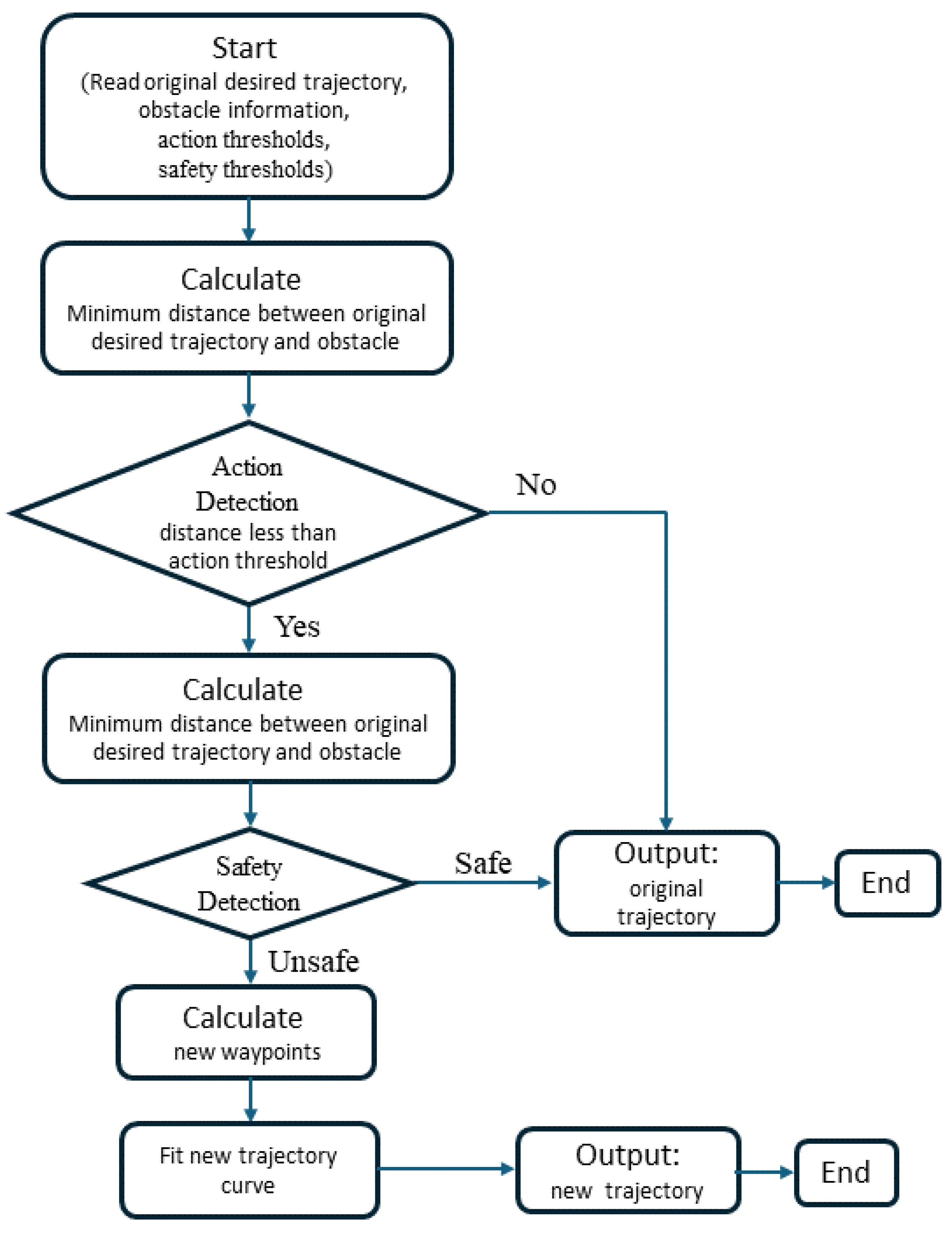
In the domain of trajectory-tracking control, it is customary to craft trajectories in advance, incorporating available environmental data. However, real-world operational environments frequently present unforeseen obstacles. As a robot nears such an obstacle, it employs sensors to ascertain the obstacle’s location and dimensions. This paper introduces a trajectory re-planning algorithm predicated on the principles of nonlinear least squares. The algorithm assesses the potential for collision between the pre-defined trajectory and any detected obstacles. Should a collision risk be identified, the algorithm is designed to autonomously generate an alternate trajectory to navigate around the obstacle safely. The flowchart presented in Figure 2 represents the specific implementation of the proposed trajectory replanning.
Inputs for the algorithm encompass the obstacle’s position and radius , current position for TTWR P, the initial trajectory T, along with predefined action and safety thresholds denoted by and , respectively. The algorithm delineated herein is bifurcated into two primary components.
Necessity Assessment for Trajectory Re-planning—The initial segment of the algorithm is devoted to ascertaining the need for trajectory modification. It proceeds as follows:
- Compute the distance L between the robot and the obstacle and evaluate whether L exceeds the movement threshold ;
- If , the robot continues along the pre-set trajectory; conversely, if , record the current time as and estimate the end time , at which the distance between the robot and the obstacle should again surpass .
- Ascertain whether there exists an instance within the interval such that at , the distance falls below the safety threshold .
- Should not exist, re-planning is deemed unnecessary; if is found, initiate re-planning of a new, secure trajectory within the active interval to supplant the original hazardous trajectory.
Trajectory Re-planning Procedure—The second component outlines the specific methodology for re-constructing the trajectory as follows:
- Define the movement vector from the position at time to the position at time as the x-axis of a safe coordinate system. Establish the y-axis per the right-hand rule, designating the obstacle’s center as the coordinate origin, as shown in Figure 3.
- Compute the rotation matrix and translation vector that characterize the safe coordinate system in relation to the inertial frame. This computation facilitates the subsequent mapping of positions and velocities at times and into the safe coordinate system, as shown in Figure 4.
- Configure the new trajectory to intersect the point (0, b) within the safe coordinate system, ensuring the y-velocity is zero and adopting the mean x-velocity from times and for the x-velocity, as shown in Figure 4.
- Integrate the data from , and the designated point to construct the new, collision-free trajectory using nonlinear fitting techniques.
- Finally, convert the newly determined trajectory from the safe coordinates back into the inertial coordinates to execute the trajectory in the robot’s operational environment, as shown in Figure 3.
Remark 3.
In trajectory re-planning, to accommodate diverse operational contexts, multiple waypoints may be employed, and the trajectory’s configuration can be tailored to the situational requirements. Standard trajectory forms encompass linear, arc, and sinusoidal paths, among others, or a hybrid of these shapes. This approach is analogous to the generation of Dubins paths [33].
2.4. Control Design
The following assumptions are made for the tractor–trailer system to facilitate the discussion of our analysis.
Assumption 1.
The system initial conditions satisfy
Remark 4.
Our study makes two primary assumptions. First, we assume no wheel slippage, which leads to nonholonomic constraints and simplifies the system model by neglecting lateral skid forces. This assumption may limit model applicability under slippery conditions. Second, as illustrated in Assumption 1, we assume initial conditions fall within safe bounds. This is crucial for the employed UBF method to ensure the system converges to the vicinity of the desired equilibrium point.
In this section, we extend the utilization of the generalized barrier function methodology, as delineated in prior work [31], to proficiently handle constraints pertinent to system performance. Initially, we introduce a transformed error variable , defined as follows:
Following this, we construct the universal barrier function (UBF) to encapsulate the performance constraints as follows:
It can be observed that is zero if and only if equals zero. Furthermore, as nears the boundary , increases unbounded towards positive infinity, which in turn causes the associated barrier function to also approach infinity. In contrast, when tends towards , decreases without bound to negative infinity, resulting in escalating to infinity.
Delving into the dynamics of , we derive the following:
Therefore, the temporal derivative of the UBF (10) is given by
where
in which is always guaranteed by its structure.
In Equation (11), the term is incorporated as the gain factor for the velocity control input v. For the proposed control strategy to remain viable, it is imperative to maintain the non-negativity of this gain. Specifically, it is required that . To satisfy this condition, the following feasibility constraint must be met:
ensuring that the angle between and does not exceed radians. This constraint is essential to preserve the directional consistency of the control input gain.
To satisfy the feasibility constraints delineated in Equation (12), we introduce a new transformed state variable z, defined as follows:
This transformation ensures that z remains a bounded signal if, and only if, the constraints specified in (12) are met. To facilitate the stability analysis, we propose the following candidate for the second Lyapunov function:
whose time derivative leads to
where
Furthermore, the term yields
Remark 5.
Then, we define the linear velocity control laws v as follows:
where the scaling factor is given by
and the angular velocity control law is
with the factor being
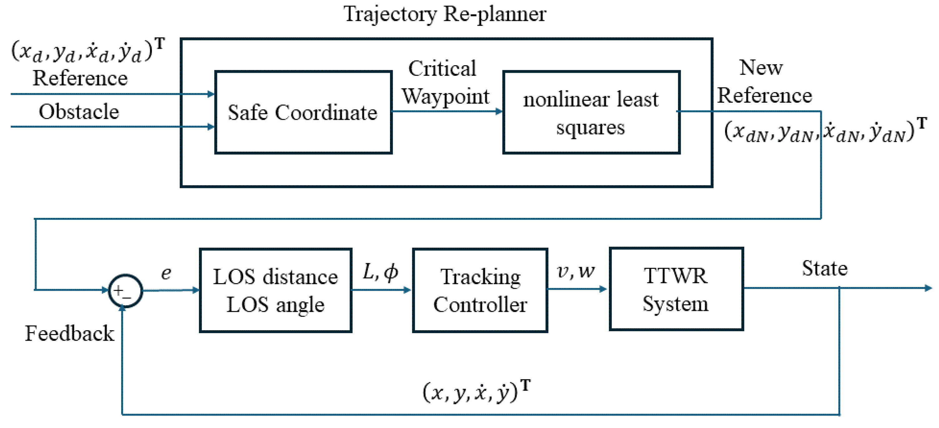
where K is a positive control gain that must be suitably chosen. The block diagram of the proposed non-linear platoon control system is given by Figure 5.
Remark 6.
The values of the positive control gains K of this work have been chosen based on the following: Larger values of K lead to faster convergence of the tracking errors, as can be seen from the Lyapunov analysis in the proof of Theorem 1. However, too large values may cause high control inputs. Thus, K is balanced between tracking performance and magnitude of control input.
We next introduce the following Lyapunov stability lemma, which will be instrumental for the subsequent proof of our main theorem.
Lemma 1
([34]). For any positive constants , let : and be open sets. Consider the system
where , and is piecewise continuous in t and locally Lipschitz in z, uniformly in t, on . Suppose that there exist functions and , continuously differentiable and positive definite in their respective domains, such that
where and are class functions. Let and belong to the set . If the inequality holds,
then remains in the open set .
Building upon the introduced lemma, we now present the proposed control law encapsulated in the theorem below.
Theorem 1.
Consider the tractor–trailer system as described by Equation (1). Under the influence of the control laws defined in Equations (17) and (19), the system exhibits the following characteristics:
- LOS Distance Tracking Error: The LOS distance tracking error, denoted as , demonstrates exponential convergence towards a small positive boundary , where is an arbitrarily chosen small positive number. This implies that the trailer’s trajectory will approximate the desired trajectory within an arbitrarily small error margin.
- Tractor Angle Convergence: The tractor’s angle, , is guaranteed to converge exponentially towards the LOS angle, , which represents the angular discrepancy between the desired trajectory and the actual position of the tractor. This ensures that the tractor’s orientation is progressively corrected to align the trailer along the desired path.
Proof.
To establish the stability of the designed control system, we introduce a composite Lyapunov function as follows:
where is as defined in Equation (10), and conforms to the definition in Equation (13). Invoking the differential relationships presented in Equations (11) and (14) and applying the prescribed control laws from Equations (17) and (18), it follows that
Similarly, by applying (15), (19) and (20), we can obtain the following result:
which gives to Based on Lemma 1, we can ascertain the stability of the system states. This implies that
In the second instance, the uniform boundedness of the Lyapunov function V allows us to deduce that both and z are uniformly bounded as well. This boundedness guarantees that the system will respect the performance constraint requirement as outlined in Equation (8) and the feasibility constraint requirement as detailed in Equation (12) throughout its operation.
Consequently, the uniform boundedness of the control laws specified in Equations (17) and (19) is evident, as all the signals involved in the design are uniformly bounded. The integrity of the system’s constraints, coupled with the bounded nature of the control inputs, affirm the robustness of the control strategy. □
Remark 7.
In the presented study, we delineate two distinct methodologies to address constraints of diverse natures within the tractor–trailer system. Initially, we employ a UBF to facilitate the examination of the performance constraint requirement, as articulated in Equation (8), specifically pertaining to the LOS distance tracking error, . The UBF approach is particularly beneficial when dealing with asymmetric constraints, where the imposed limits exhibit unequal magnitudes on either side of the equilibrium. This technique enables a consolidated framework for accommodating such disparities in constraint bounds.
Subsequently, we introduce an innovative state transformation strategy to analyze the feasibility constraint requirement, detailed in Equation (12), that governs the heading angles within the tractor–trailer system. Distinct from the UBF method—which is restricted to managing a single variable under constraint for each UBF—our proposed state transformation adeptly encapsulates multiple constrained variables into a unified analysis framework. In the context of our work, the state transformation facilitates the concurrent analysis of both tractor and trailer heading angles, denoted as and , respectively, by converting them into a single transformed state variable, z. This novel approach significantly streamlines the analytical process, allowing for a more cohesive and efficient examination of constraints pertaining to multiple state variables.
3. Results
3.1. Trajectory Tracking
To evaluate the efficacy of the proposed control architecture, a suite of simulations was performed within the MATLAB framework. We set the link length between vehicles, d, to 1.5 m. The intended path for the trailer was delineated by specific equations as follows:
For the performance constraints, we established the upper bound as and the lower bound as . This configuration necessitates that the distance tracking error L be confined within an exponentially decreasing envelope to ensure accurate tracking, while also being maintained above a minimal positive value to circumvent singularities.
The control gain K was set at . Initial states for the tractor–trailer system were assigned as follows: , , , , , and .
The simulation results are depicted in Figure 6, Figure 7, Figure 8 and Figure 9. Figure 6 illustrates the trajectories of both the tractor and trailer in relation to the desired trajectory, demonstrating the tracking proficiency of the proposed control system. The outcomes reveal that the tractor–trailer system promptly aligns with the desired trajectory, exhibiting notable tracking precision.
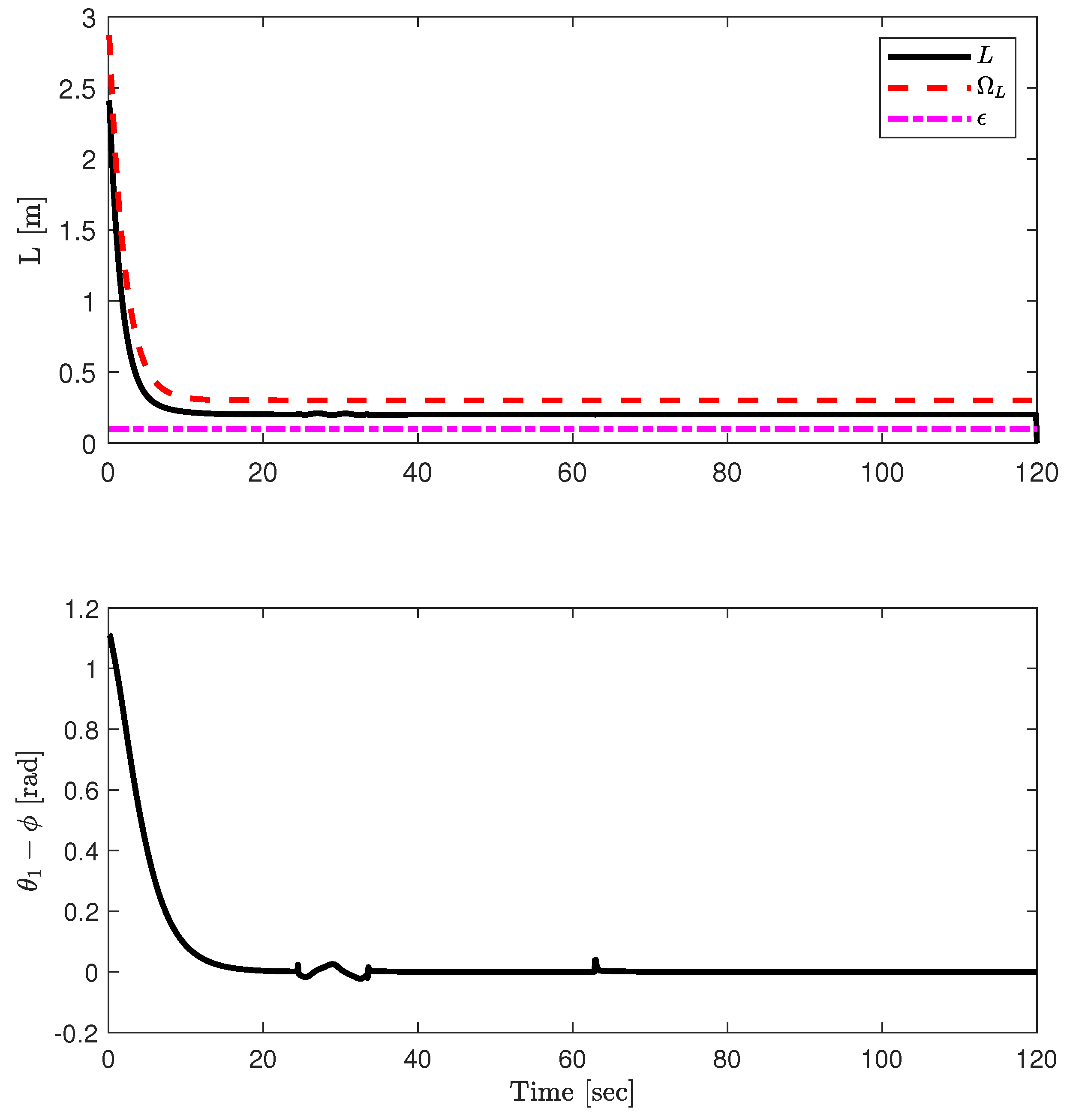
Figure 7 exhibits the tractor’s distance tracking error and heading angle tracking error. The top panel illustrates the correlation between the distance tracking error and the constraint boundary and , confirming that satisfies the constraint over the entire time scale. The bottom panel depicts the temporal variation in the LOS angle error , evaluating the dynamics of the angle error and its convergence behavior.
Figure 8 presents the distance tracking error and heading angle tracking error for the trailer. The upper section delineates the distance discrepancy between the actual and target positions, while the lower section exhibits the angular deviation between the actual and desired heading angles .
Additionally, the control inputs for the system are presented in Figure 9. Collectively, these simulation results empirically substantiate the theoretical claims put forth in Theorem 1.
3.2. Avoid Obstacles
To ascertain the effectiveness of the proposed trajectory re-planning algorithm, we incorporate a circular obstacle with coordinates and a radius of 1 into the tracking-control simulation scenario described in the preceding section. The movement and safety thresholds applied within the simulation are set to and , respectively.
For the performance constraints, we specify the upper bound and the lower bound . This implies that the distance tracking error L is constrained by an exponentially decaying function to guarantee precise tracking, while adopting a small positive constant as a lower bound is employed as the lower bound to preclude issues related to singularity. The control gain K is determined to be . Initial conditions were prescribed for the tractor–trailer system as follows: , , , , , and .
The simulation results for the obstacle avoidance problem are depicted in Figure 10, Figure 11 and Figure 12. Figure 10 compares the control law from the literature [30,31] with the control strategy proposed in this study; the latter demonstrates superior responsiveness and faster alignment with the desired trajectory.
Figure 11 illustrates the distance tracking error and heading angle tracking error for the tractor. The upper plot portrays the relationship between the distance error and the constraint boundaries and ; the lower plot shows the variation of the LOS angle error .
Figure 12 displays the control inputs. Collectively, the results validate the effectiveness of the re-planning algorithm and the tracking control law.
4. Discussion
In practical implementation, the collision avoidance strategy employed in this work relies on maintaining a specified distance from obstacles. While our decoupled approach to planning and control accelerates computational speed, it fails to guarantee optimal solutions. Therefore, pursuing integrated planning and control algorithms that address these issues concurrently represents a promising direction for future research.
Regarding motion control, the proposed control law demonstrates commendable transient performance in simulations but lacks the desired smoothness in response. The simulation system is overly simplified, neglecting real-world nonlinearities such as input delays and actuator saturation, which are crucial for actual deployment. These elements will be central to our future research endeavors.
Several potential challenges arise when implementing the proposed control law on an actual tractor–trailer wheeled-robot system.
- State Feedback and Sensor Noise: Full state feedback requires precise measurements of position, orientation, and velocity, which are susceptible to noise from onboard sensors. The implementation of filtering and sensor fusion techniques is vital for accurate state estimation.
- Actuation Constraints: The control law assumes unrestricted steering angles and velocities, whereas physical robots have inherent limitations. Command inputs must be saturated within practical bounds. Model Predictive Control (MPC) presents a promising solution to such constraint issues. However, these methods often rely on numerical optimization to derive control laws, thus analytical guarantees of stability cannot be ensured.
- Parameter Uncertainty and Disturbances: Fixed model parameters, such as wheel radius and hitch length, are subject to variations in the physical environment, and disturbances like uneven terrain can affect the system behavior. Robust or adaptive control methods could provide compensation for these uncertainties.
The theoretical framework of the control law is promising, but substantial work is required to address real-world issues such as sensor noise, actuator limitations, parameter uncertainty, and external disturbances. Through careful modeling and robust design, the control approach can be adapted to real-world tractor–trailer systems, and extensive testing and validation prior to actual deployment are crucial.
5. Conclusions
This study introduces a novel TTWR trajectory tracking control framework, comprising a trajectory replanner and a tracking controller. Specifically, the desired trajectory for the tractor is derived based on the trailer’s desired trajectory and the system’s internal constraints. The trajectory replanner then employs coordinate transformations and nonlinear least squares techniques to generate a new desired tracking trajectory for the tractor. Stability analysis is conducted using UBF, based on the performance requirements of the Line-of-Sight (LOS) tracking error between the actual and desired tractor trajectory. A novel state transformation approach addresses constraints related to the vehicle’s heading angle, ensuring that both LOS distance and angle tracking errors exponentially converge to a small neighborhood of equilibrium. Simulation results demonstrate that the proposed controller outperforms previous studies in transient characteristics. Future work will explore the incorporation of time-delay compensation and noise/disturbance suppression into the control design, aiding in experimental testing on physical platforms.
Author Contributions
Conceptualization, Y.Z.; methodology, T.Z.; software, Y.Y.; validation, T.Z., Y.Y. and P.L.; investigation, P.L.; formal analysis, L.Z.; writing—original draft preparation, T.Z. and Y.Y.; visualization, T.Z. and Y.Y.; writing—review and editing, T.Z. and Y.Y. All authors have read and agreed to the published version of the manuscript.
Funding
This work is supported by the projects of National Natural Science Foundation of China (U2033208), School-Enterprise collaboration project (SA0202107), China Postdoctoral Science Foundation (2023M742265), Natural Science Foundation of Chongqing (2023NSCQ-MSX0758), and Science and Technology Research Program of Chongqing Municipal Education Commission (KJZD-K202301403).
Institutional Review Board Statement
Not applicable.
Informed Consent Statement
Not applicable.
Data Availability Statement
Data are contained within the article.
Conflicts of Interest
The authors declare no conflict of interest.
Abbreviations
The following abbreviations are used in this manuscript:
| TTWR | Tractor–Trailer Wheeled Robot |
| LOS | line of sight |
| UBF | Universal Barrier Function |
| CBF | Control Barrier Function |
Appendix A
References
- Astolfi, A.; Bolzern, P.; Locatelli, A. Path-tracking of a tractor-trailer vehicle along rectilinear and circular paths: A Lyapunov-based approach. IEEE Trans. Robot. Autom. 2004, 20, 154–160. [Google Scholar] [CrossRef]
- Kassaeiyan, P.; Alipour, K.; Tarvirdizadeh, B. A full-state trajectory tracking controller for tractor-trailer wheeled mobile robots. Mech. Mach. Theory 2020, 150, 103872. [Google Scholar] [CrossRef]
- Yuan, J.; Sun, F.; Huang, Y. Trajectory generation and tracking control for double-steering tractor–trailer mobile robots with on-axle hitching. IEEE Trans. Ind. Electron. 2015, 62, 7665–7677. [Google Scholar] [CrossRef]
- Leng, Z.; Minor, M.A. Curvature-based ground vehicle control of trailer path following considering sideslip and limited steering actuation. IEEE Trans. Intell. Transp. Syst. 2016, 18, 332–348. [Google Scholar] [CrossRef]
- Lashkari, N.; Biglarbegian, M.; Yang, S.X. Backstepping tracking control design for a tractor robot pulling multiple trailers. In Proceedings of the 2018 Annual American Control Conference (ACC), Milwaukee, WI, USA, 27–29 June 2018; pp. 2715–2720. [Google Scholar]
- Elhaki, O.; Shojaei, K. Output-feedback robust saturated actor–critic multi-layer neural network controller for multi-body electrically driven tractors with n-trailer guaranteeing prescribed output constraints. Robot. Auton. Syst. 2022, 154, 104106. [Google Scholar] [CrossRef]
- Elhaki, O.; Shojaei, K. Observer-based neural adaptive control of a platoon of autonomous tractor–trailer vehicles with uncertain dynamics. IET Control. Theory Appl. 2020, 14, 1898–1911. [Google Scholar] [CrossRef]
- Beglini, M.; Lanari, L.; Oriolo, G. Anti-jackknifing control of tractor-trailer vehicles via intrinsically stable MPC. In Proceedings of the 2020 IEEE International Conference on Robotics and Automation (ICRA), Paris, France, 31 May–31 August 2020; pp. 8806–8812. [Google Scholar]
- Beglini, M.; Belvedere, T.; Lanari, L.; Oriolo, G. An intrinsically stable MPC approach for anti-jackknifing control of tractor-trailer vehicles. IEEE/ASME Trans. Mechatron. 2022, 27, 4417–4428. [Google Scholar] [CrossRef]
- Kassaeiyan, P.; Tarvirdizadeh, B.; Alipour, K. Control of tractor-trailer wheeled robots considering self-collision effect and actuator saturation limitations. Mech. Syst. Signal Process. 2019, 127, 388–411. [Google Scholar] [CrossRef]
- Ezeddin, L.M.H.; Mohmmadion, A. Trajectory tracking weeled mobile robot using backstepping method with connection off axle trailer. Int. J. Smart Electr. Eng. 2018, 7, 177–187. [Google Scholar]
- Jalalnezhad, M.; Fazeli, S.; Bozorgomid, S.; Ghadimi, M. Stability and control of the nonlinear system for tractor with N trailer in the presence of slip. Adv. Mech. Eng. 2021, 13, 16878140211047745. [Google Scholar] [CrossRef]
- Khalaji, A.K.; Moosavian, S.A.A. Robust adaptive controller for a tractor–trailer mobile robot. IEEE/ASME Trans. Mechatron. 2013, 19, 943–953. [Google Scholar] [CrossRef]
- Khalaji, A.K.; Moosavian, S.A.A. Stabilization of a tractor-trailer wheeled robot. J. Mech. Technol. 2016, 30, 421–428. [Google Scholar] [CrossRef]
- Khalaji, A.K.; Jalalnezhad, M. Stabilization of a Tractor with n Trailers in the Presence of Wheel Slip Effects. Robotica 2021, 39, 787–797. [Google Scholar] [CrossRef]
- Van Hau, P.; Nam, D.P.; Ha, N.T.; Thanh, P.T.; Hai, H.T.; Hanh, H.D. Asymptotic stability of the whole tractor-trailer control system. In Proceedings of the 2017 International Conference on System Science and Engineering (ICSSE), Ho Chi Minh City, Vietnam, 21–23 July 2017; pp. 423–427. [Google Scholar]
- Yu, M.; Gong, X.; Fan, G.; Zhang, Y. Trajectory Planning and Tracking for Carrier Aircraft-Tractor System Based on Autonomous and Cooperative Movement. Math. Probl. Eng. 2020, 2020, 6531984. [Google Scholar] [CrossRef]
- Yin, C.; Wang, S.; Li, X.; Yuan, G.; Jiang, C. Trajectory tracking based on adaptive sliding mode control for agricultural tractor. IEEE Access 2020, 8, 113021–113029. [Google Scholar] [CrossRef]
- Kayacan, E.; Kayacan, E.; Ramon, H.; Saeys, W. Nonlinear modeling and identification of an autonomous tractor–trailer system. Comput. Electron. Agric. 2014, 106, 1–10. [Google Scholar] [CrossRef]
- Kim, D.H.; Oh, J.H. Nonlinear tracking control of trailer systems using the Lyapunov direct method. J. Robotic Syst. 1999, 16, 1–8. [Google Scholar] [CrossRef]
- Zhou, B. Lyapunov differential equations and inequalities for stability and stabilization of linear time-varying systems. Automatica 2021, 131, 109785. [Google Scholar] [CrossRef]
- Zhang, K.K.; Zhou, B.; Hou, M.; Duan, G.R. Prescribed-time stabilization of p-normal nonlinear systems by bounded time-varying feedback. Int. J. Robust Nonlinear Control 2022, 32, 421–450. [Google Scholar] [CrossRef]
- Hassan, N.; Saleem, A. Neural network-based adaptive controller for trajectory tracking of wheeled mobile robots. IEEE Access 2022, 10, 13582–13597. [Google Scholar] [CrossRef]
- Xu, P.; Cui, Y.; Shen, Y.; Zhu, W.; Zhang, Y.; Wang, B.; Tang, Q. Reinforcement learning compensated coordination control of multiple mobile manipulators for tight cooperation. Eng. Artif. Intell. 2023, 123, 106281. [Google Scholar] [CrossRef]
- Khanpoor, A.; Khalaji, A.K.; Moosavian, S.A.A. Modeling and control of an underactuated tractor–trailer wheeled mobile robot. Robotica 2017, 35, 2297–2318. [Google Scholar] [CrossRef]
- Naderolasli, A.; Shojaei, K.; Chatraei, A. Leader-follower formation control of Euler–Lagrange systems with limited field-of-view and saturating actuators: A case study for tractor-trailer wheeled mobile robots. Eur. J. Control 2023, 75, 100903. [Google Scholar] [CrossRef]
- Binh, N.T.; Tung, N.A.; Nam, D.P.; Quang, N.H. An adaptive backstepping trajectory tracking control of a tractor trailer wheeled mobile robot. Int. J. Control Autom. Syst. 2019, 17, 465–473. [Google Scholar] [CrossRef]
- Yue, M.; Hou, X.; Gao, R.; Chen, J. Trajectory tracking control for tractor-trailer vehicles: A coordinated control approach. Nonlinear Dyn. 2018, 91, 1061–1074. [Google Scholar] [CrossRef]
- Aro, K.; Urvina, R.; Deniz, N.N.; Menendez, O.; Iqbal, J.; Prado, A. A Nonlinear Model Predictive Controller for Trajectory Planning of Skid-Steer Mobile Robots in Agricultural Environments. In Proceedings of the 2023 IEEE Conference on AgriFood Electronics (CAFE), Torino, Italy, 25–27 September 2023; pp. 65–69. [Google Scholar]
- Jin, X.; Dai, S.L.; Liang, J.; Guo, D.; Tan, H. Constrained line-of-sight tracking control of a tractor-trailer mobile robot system with multiple constraints. In Proceedings of the 2021 American Control Conference (ACC), New Orleans, LA, USA, 25–28 May 2021; pp. 1046–1051. [Google Scholar]
- Jin, X.; Liang, J.; Dai, S.L.; Guo, D. Adaptive Line-of-Sight tracking control for a tractor-trailer vehicle system with multiple constraints. IEEE Trans. Intell. Transp. 2021, 23, 11349–11360. [Google Scholar] [CrossRef]
- Jin, X.; Dai, S.L.; Liang, J. Adaptive constrained formation-tracking control for a tractor-trailer mobile robot team with multiple constraints. IEEE Trans. Autom. Control 2022, 68, 1700–1707. [Google Scholar] [CrossRef]
- Shkel, A.M.; Lumelsky, V. Classification of the Dubins set. Robot. Auton. Syst. 2001, 34, 179–202. [Google Scholar] [CrossRef]
- Tee, K.P.; Ge, S.S.; Tay, E.H. Barrier Lyapunov functions for the control of output-constrained nonlinear systems. Automatica 2009, 45, 918–927. [Google Scholar] [CrossRef]
Figure 1.
Schematics of the tracking-control problem for the TTWR system.

Figure 2.
Flowchart of trajectory re-planner algorithm.

Figure 3.
Inertial coordinate trajectory re-planning schematic.

Figure 4.
Safe coordinate trajectory re-planning schematic.

Figure 5.
A block diagram of the platoon control system.

Figure 6.
(a) The Desired path and (b) phase-plane trajectories of the TTWR.

Figure 7.
Tractor LOS distance and angle tracking error.

Figure 8.
Trailer tracking performance.

Figure 9.
The profile of the velocity control inputs applied to the tractor.

Figure 10.
Phase -plane trajectories of the TTWR for obstacle avoidance problem using control laws (a) proposed in literature [30,31] and (b) introduced in this paper.

Figure 11.
Tractor LOS distance and angle tracking error.

Figure 12.
The profile of the velocity control inputs applied to the tractor.

Disclaimer/Publisher’s Note: The statements, opinions and data contained in all publications are solely those of the individual author(s) and contributor(s) and not of MDPI and/or the editor(s). MDPI and/or the editor(s) disclaim responsibility for any injury to people or property resulting from any ideas, methods, instructions or products referred to in the content. |
© 2024 by the authors. Licensee MDPI, Basel, Switzerland. This article is an open access article distributed under the terms and conditions of the Creative Commons Attribution (CC BY) license (https://creativecommons.org/licenses/by/4.0/).
Share and Cite
MDPI and ACS Style
Zhao, T.; Li, P.; Yuan, Y.; Zhang, L.; Zhao, Y. Trajectory Re-Planning and Tracking Control for a Tractor–Trailer Mobile Robot Subject to Multiple Constraints. Actuators 2024, 13, 109. https://0-doi-org.brum.beds.ac.uk/10.3390/act13030109
AMA Style
Zhao T, Li P, Yuan Y, Zhang L, Zhao Y. Trajectory Re-Planning and Tracking Control for a Tractor–Trailer Mobile Robot Subject to Multiple Constraints. Actuators. 2024; 13(3):109. https://0-doi-org.brum.beds.ac.uk/10.3390/act13030109
Chicago/Turabian StyleZhao, Tianrui, Peibo Li, Yu Yuan, Lin Zhang, and Yanzheng Zhao. 2024. "Trajectory Re-Planning and Tracking Control for a Tractor–Trailer Mobile Robot Subject to Multiple Constraints" Actuators 13, no. 3: 109. https://0-doi-org.brum.beds.ac.uk/10.3390/act13030109
Note that from the first issue of 2016, this journal uses article numbers instead of page numbers. See further details here.