Bivariate Assessment of Drought Return Periods and Frequency in Brazilian Northeast Using Joint Distribution by Copula Method

 , , and
Abstract
:1. Introduction
2. Materials and Methods
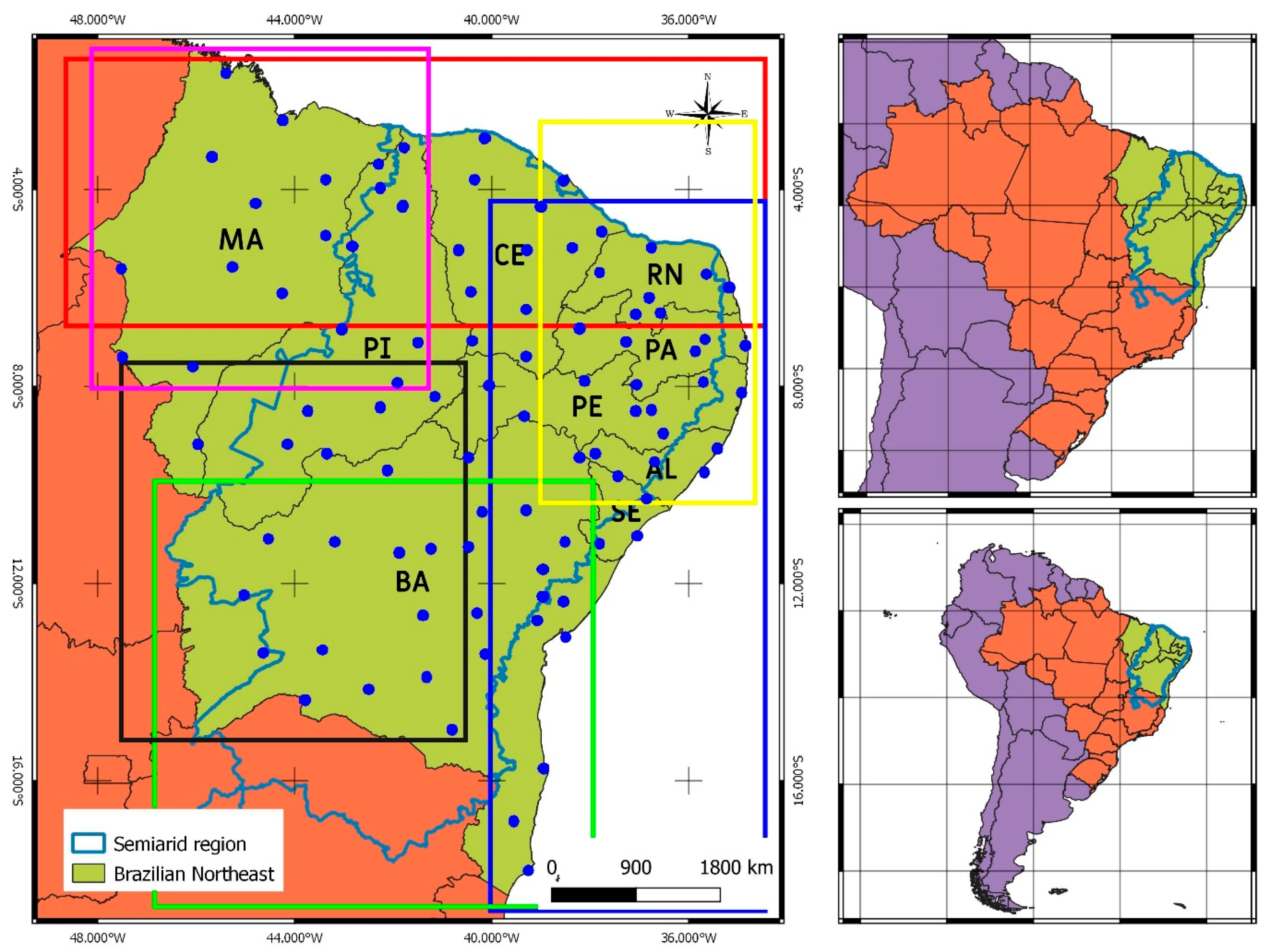
2.1. Data and Area of Study
2.2. Standardized Precipitation Index
2.3. Bivariate Copula
2.4. Marginal Distribuitions for Drought Severity and Duration
2.5. Return Period Estimation
3. Results and Discussion
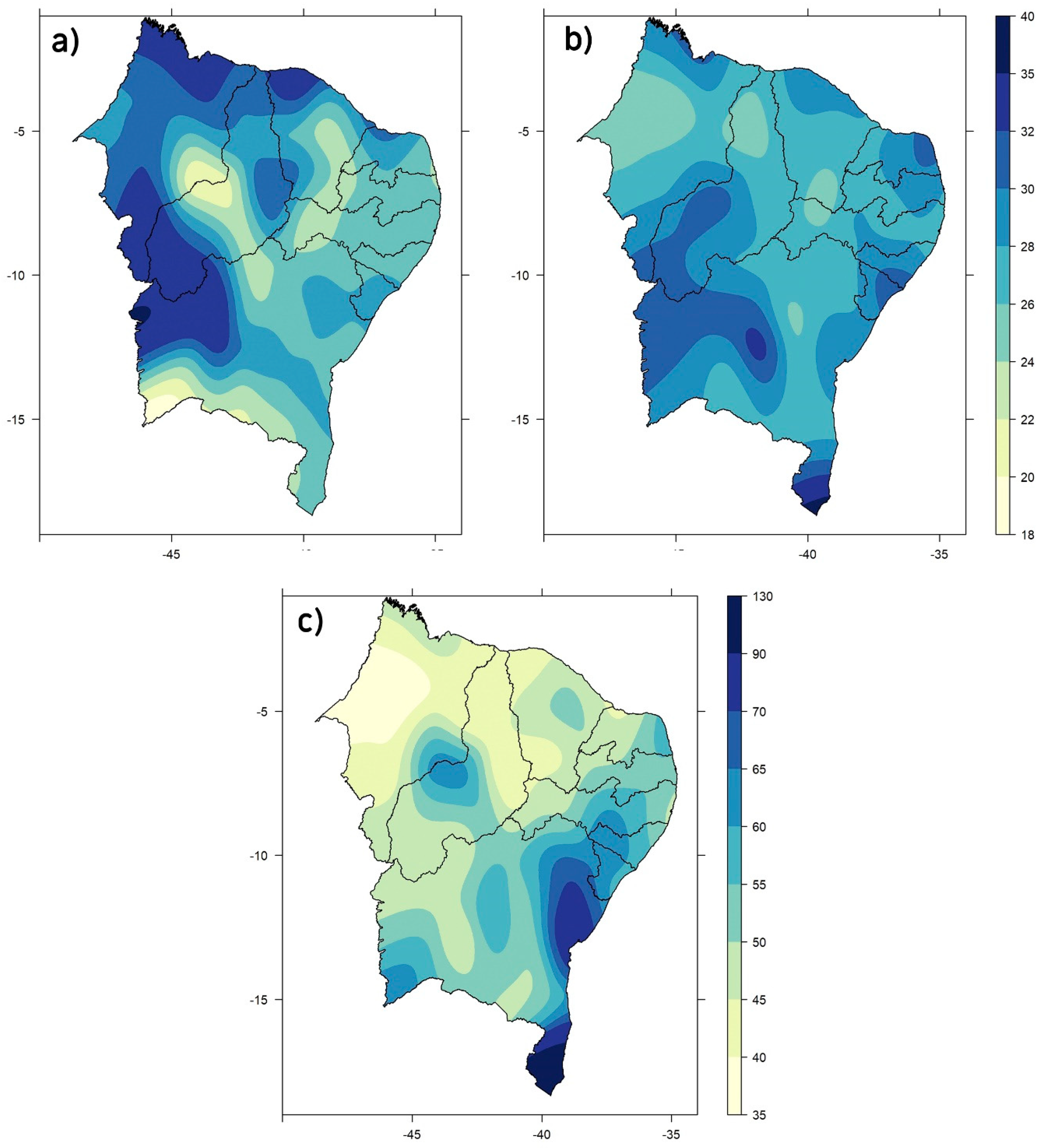
3.1. Drought Frequency
3.2. Marginal Distributions
3.3. Bivariate Joint Probability Distribution
3.4. Return Period
4. Conclusions
Author Contributions
Funding
Acknowledgments
Conflicts of Interest
References
- Marengo, J.A.; Torres, R.R.; Alves, L.M. Drought in Northeast Brazil-past, present, and future. Theor. Appl. Climatol. 2016, 129, 1189–1200. [Google Scholar] [CrossRef]
- Wilhite, D.A.; Glantz, M.H. Understanding the Drought Phenomenon: The Role of Definitions. Water Int. 1985, 10, 111–120. [Google Scholar] [CrossRef] [Green Version]
- Cunha, A.P.M.A.; Alvalá, R.C.S.; Nobre, C.A.; Carvalho, M.A. Monitoring vegetative drought dynamics in the Brazilian semiarid Region. Agric. For. Meteorol. 2015, 214, 494–505. [Google Scholar] [CrossRef]
- Cunha, A.P.M.A.; Tomasella, J.; Ribeiro-Neto, G.G.; Brown, M.; Garcia, S.R.; Brito, S.B.; Carvalho, M.A. Changes in the spatial-temporal patterns of droughts in the Brazilian Northeast. Atmos. Sci. Lett. 2018, 19, e855. [Google Scholar] [CrossRef] [Green Version]
- Cunha, A.P.M.A.; Zeri, M.; Leal, K.D.; Costa, L.; Cuartas, L.A.; Marengo, J.A.; Tomasella, J.; Vieira, R.M.; Barbosa, A.A.; Cunningham, C.; et al. Extreme Drought Events over Brazil from 2011 to 2019. Atmosphere 2019, 10, 642. [Google Scholar] [CrossRef] [Green Version]
- Alvala, R.C.S.; Cunha, A.P.M.A.; Brito, S.S.B.; Seluchi, M.E.; Marengo, J.A.; Moraes, O.L.L.; Carvalho, M.A. Drought monitoring in the Brazilian Semiarid region. An. Acad. Bras. Ciências 2017, 91, 1–15. [Google Scholar] [CrossRef] [PubMed] [Green Version]
- Martins, E.S.P.R.; Coelho, C.A.S.; Haarsma, R.; Otto, F.E.L.; King, A.D.; Van Oldenborgh, G.J.; Kew, S.; Philip, S.; Júnior, F.C.V.; Cullen, H. A multimethod attribution analysis of the prolonged northeast Brazil hydrometeorological drought (2012–16). Bull. Am. Meteorol. Soc. 2018, 99, 65–69. [Google Scholar] [CrossRef]
- Martins, M.A.; Tomasella, J.; Rodriguez, D.A.; Alvalá, R.C.; Giarolla, A.; Garofolo, L.L.; Júnior, J.L.S.; Paolicchi, L.T.; Pinto, G.L. Improving droughtmanagement in the Brazilian semiarid through crop forecasting. Agric. Syst. 2018, 160, 21–30. [Google Scholar] [CrossRef]
- Vincente-Serrano, S.M.; Beguería, S.; López-Moreno, J.I.; Angulo, M.; Kenawy, A.E. A new global 0.5 degrees gridded dataset (1901–2006) of a multiscalar drought index: Comparison with current drought index datasets based on the Palmer Drought Severity Index. J. Hydrometeorol. 2010, 11, 1033–1043. [Google Scholar] [CrossRef] [Green Version]
- Finan, T.J.; Nelson, D. Making Rain, Making Roads, Making Do: Public and Private Adaptations to Drought in Ceará, Northeast Brazil. Clim. Res. 2001, 19, 97–108. [Google Scholar] [CrossRef]
- Spinoni, J.; Antofie, T.; Barbosa, P.; Bihari, Z.; Lakatos, M.; Szalai, S.; Szentimrey, T.; Vogt, J. An overview of drought events in the Carpathian region in 1961–2010. Adv. Sci. Res 2013, 10, 21–32. [Google Scholar] [CrossRef] [Green Version]
- Sinopse do Censo Demográfico 2010; Instituto Brasieliro de Geografia e Estatística-IBGE: Rio de Janeiro, Brazil, 2010. Available online: https://biblioteca.ibge.gov.br/index.php/biblioteca-catalogo?view=detalhes&id=249230 (accessed on 9 April 2020).
- Eakin, H.C.; Lemos, M.C.; Nelson, D.R. Differentiating capacities as a means to sustainable climate change adaptation. Glob. Environ. Chang. 2014, 27, 1–8. [Google Scholar] [CrossRef]
- Salvador, M.A.; de Brito, J.I.B. Trend of annual temperature and frequency of extreme events in the MATOPIBA region of Brazil. Theor. Appl. Climatol. 2018, 133, 253–261. [Google Scholar] [CrossRef]
- Namias, J. Influence of northern hemisphere general circulation on drought in northeast Brazil. Tellus XXIV 1972, 4, 336–343. [Google Scholar]
- Hastenrath, S.; Heller, L. Dynamics of climatic hazards in northeast Brazil. Q. J. R. Meteorol. Soc. 1977, 103, 77–92. [Google Scholar] [CrossRef]
- Moura, A.D.; Shukla, J. On the dynamics of droughts in northeast Brazil: Observations, theory and numerical experiments with a general circulation model. J. Atmos. Sci. 1981, 38, 2653–2675. [Google Scholar] [CrossRef] [Green Version]
- Hastenrath, S. Circulation and teleconnection mechanisms of Northeast Brazil droughts. Prog. Oceanogr. 2006, 70, 407–415. [Google Scholar] [CrossRef]
- Kucharski, F.; Polzin, D.; Hastenrath, S. Teleconnection Mechanisms of Northeast Brazil Droughts: Modeling and Empirical Evidence. Rev. Bras. De Meteorol. 2008, 23, 115–125. [Google Scholar] [CrossRef] [Green Version]
- Marengo, J.A.; Alves, L.M.; Soares, W.R.; Rodriguez, D.A.; Camargo, H.; Riveros, M.P.; Pabló, A.D. Two contrasting severe seasonal extremes in Tropical South America in 2012: Floods in Amazonia and Drought in Northeast Brazil. J. Clim. 2013, 26, 9137–9154. [Google Scholar] [CrossRef]
- Lemos, M.C.; Finan, T.J.; Fox, R.W.; Nelson, D.R.; Tucker, J. The Use of Seasonal Climate Forecasting in Policymaking: Lessons from Northeast Brazil. Clim. Chang. 2002, 55, 479–507. [Google Scholar] [CrossRef]
- Nelson, D.R.; Finan, T.J. Praying for Drought: Persistent Vulnerability and the Politics of Patronage in Ceará, Northeast Brazil. Am. Anthropol. 2009, 111, 302–316. [Google Scholar] [CrossRef]
- Costa, D.D.; Pereira, T.A.S.; Fragoso, C.R., Jr.; Madani, K.; Uvo, C.B. Understanding Drought Dynamics during Dry Season in Eastern Northeast Brazil. Front. Earth Sci. 2016, 4, 69. [Google Scholar] [CrossRef]
- Brito, S.S.B.; Cunha, A.P.M.A.; Cunningham, C.C.; Alvalá, R.C.; Marengo, J.A.; Carvalho, M.A. Frequency, duration and severity of drought in the Semiarid Northeast Brazil region. Int. J. Climatol. 2017, 38, 517–529. [Google Scholar] [CrossRef]
- Awange, J.; Mpelasoka, F.; Goncalves, R. When every drop counts: Analysis of droughts in Brazil for the 1901–2013 period. Sci. Total Environ. 2016, 566–567, 1472–1488. [Google Scholar] [CrossRef] [PubMed] [Green Version]
- Cancelliere, A.; Salas, J.D. Drought probabilities and return period for annual streamflows series. J. Hydrol. 2010, 391, 77–89. [Google Scholar] [CrossRef]
- Kim, T.; Valdes, J.B.; Yoo, C. Nonparametric approach for estimating return periods of droughts in arid regions. J. Hydrol. Eng. 2003, 8, 237–246. [Google Scholar] [CrossRef] [Green Version]
- Hong, X.; Guo, S.; Xiong, L.; Liu, Z. Spatial and temporal analysis of drought using entropy-based standardized precipitation index: A case study in Poyang Lake basin, China. Theor. Appl Clim. 2015, 122, 543–556. [Google Scholar] [CrossRef]
- Xu, X.; Xie, F.; Zhou, X. Research on spatial and temporal characteristics of drought based on GIS using remote sensing big data. Clust. Comput. 2016, 19, 757–767. [Google Scholar] [CrossRef]
- Chebana, F.; Ouarda, T. Multivariate quantiles in hydrological frequency analysis. Environmetrics 2011, 22, 63–78. [Google Scholar] [CrossRef] [Green Version]
- Xu, K.; Yang, D.; Xu, X.; Lei, H. Copula based drought frequency analysis considering the spatio-temporal variability in Southwest China. J. Hydrol. 2015, 527, 630–640. [Google Scholar] [CrossRef]
- Ayantobo, O.O.; Li, Y.; Song, S.; Javed, T.; Yao, N. Probabilistic modelling of drought events in China via 2-dimensional joint copula. J. Hydrol. 2018, 559, 373–391. [Google Scholar] [CrossRef]
- Wang, R.; Zhao, C.; Zhang, J.; Guo, E.; Li, D.; Alu, S.; Ha, S.; Dong, Z. Bivariate copula function-based spatial-temporal characteristics analysis of drought in Anhui Province, China. Meteorol. Atmos. Phys. 2018, 131, 1341–1355. [Google Scholar] [CrossRef]
- Hui-Mean, F.; Yusof, F.; Yusop, Z.; Suhaila, J. Trivariate copula in drought analysis: A case study in peninsular Malaysia. Theor. Appl. Climatol. 2019, 138, 657–671. [Google Scholar] [CrossRef]
- da Rocha Júnior, R.L.; dos Santos Silva, F.D.; Lisboa Costa, R.; Barros Gomes, H.; Herdies, D.L.; Rodrigues da Silva, V.P.; Candido Xavier, A. Analysis of the Space-Temporal Trends of Wet Conditions in the Different Rainy Seasons of Brazilian Northeast by Quantile Regression and Bootstrap Test. Geosciences 2019, 9, 457. [Google Scholar] [CrossRef] [Green Version]
- Filho, T.K.; Assad, E.D.; Lima, P.R.S.R. Regiões pluviometricamente homogêneas no Brasil. Pesqui. Agropecu. Bras. 2005, 40, 311–322. [Google Scholar] [CrossRef]
- Cavalcanti, I.F.A.; Ferreira, N.J.; Silva, M.G.A.J.; Dias, M.A.F.S. Tempo e Clima no Brasil; Oficina de Textos: São Paulo, Brazil, 2009. [Google Scholar]
- Marengo, J.A.; Alves, L.M.; Alvala, R.C.C.; Cunha, A.P.M.A.; Brito, S.B.; Moraes, O.L.L. Climatic characteristics of the 2010–2016 drought in the semiarid Northeast Brazil region. An. Acad. Bras. Ciências 2018, 90, 1973–1985. [Google Scholar] [CrossRef]
- Kousky, V.E. Frontal Influences on Northeast Brazil. Mon. Weather Rev. 1979, 107, 1140–1153. [Google Scholar] [CrossRef] [Green Version]
- Kousky, V.E.; Gan, M.A. Upper tropospheric cyclonic vortices in the tropical South Atlantic. Tellus 1981, 33, 538–551. [Google Scholar] [CrossRef] [Green Version]
- Costa, R.L.; De Souza, E.P.; Silva, F.D.D.S. Aplicação de uma teoria termodinâmica no estudo de um Vórtice Ciclônico de Altos Níveis sobre o nordeste do Brasil. Rev. Bras. Meteorol. 2014, 29, 96–104. [Google Scholar] [CrossRef] [Green Version]
- Cordeiro, E.S.; Fedorova, N.; Levit, V. Synoptic and thermodynamic analysis of events with thunderstorms for alagoas state in a period of 15 years (1998–2012). Rev. Bras. Meteorol. 2018, 33, 685–694. [Google Scholar] [CrossRef] [Green Version]
- De Carvalho, M.; Ângelo, V.; Oyama, M.D. Variabilidade da largura e intensidade da Zona de Convergência Intertropical atlântica: Aspectos observacionais. Rev. Bras. Meteorol. 2013, 28, 305–316. [Google Scholar] [CrossRef]
- Silva, V.B.S.; Kousky, V.E.; Silva, F.D.S.; Salvador, M.A.; Aravequia, J.A. The 2012 severe drought over Northeast Brazil. Bull. Am. Meteorol. Soc. 2013, 94, 162. [Google Scholar]
- Gomes, H.B.; Ambrizzi, T.; Herdies, D.L.; Hodges, K.; Da Silva, B.F.P. Rcio Easterly Wave Disturbances over Northeast Brazil: An Observational Analysis. Adv. Meteorol. 2015, 2015, 176238. [Google Scholar] [CrossRef] [Green Version]
- Gomes, H.B.; Ambrizzi, T.; Da Silva, B.F.P.; Hodges, K.; Dias, P.L.S.; Herdies, D.L.; Silva, M.C.L.; Gomes, H.B. Climatology of easterly wave disturbances over the tropical South Atlantic. Clim. Dyn. 2019, 53, 1393–1411. [Google Scholar] [CrossRef] [Green Version]
- Aguilar, E.; Auer, I.; Brunet, M.; Peterson, T.C.; Wieringa, J. Guidelines on Climate Metadata and Homogenization; World Meteorological Organization: Geneva, Switzerland, 2003; p. 55. [Google Scholar]
- Aguilar, E.; Peterson, T.C.; Ramírez Obando, P.; Frutos, R.; Retana, J.A.; Solera, M.; González Santos, I.; Araujo, R.M.; Rosa García, A.; Valle, V.E.; et al. Changes in precipitation and temperature extremes in Central America and northern South America, 1961–2003. J. Geophys. Res. 2005, 110, D23107. [Google Scholar] [CrossRef]
- Aguilar, E.; AzizBarry, A.; Brunet, M.; Ekang, L.; Fernandes, A.; Massoukina, M.; Mbah, J.; Mhanda, A.; do Nascimento, D.J.; Peterson, T.C.; et al. Changes in temperature and precipitation extremes in western central Africa, Guinea Conakry, and Zimbabwe 1955–2006. J. Geophys. Res 2009, 114, D02115. [Google Scholar] [CrossRef]
- Diniz, F.A.; Ramos, A.M.; Rebello, E.R.G. Brazilian climate normals for 1981–2010. Pesqui. Agropecu. Bras. 2018, 53, 131–143. [Google Scholar] [CrossRef]
- Costa, R.L.; Baptista, G.M.M.; Gomes, H.B.; Silva, F.D.S.; da Rocha Júnior, R.L.; Salvador, M.A.; Herdies, D.L. Analysis of climate extremes indices over northeast Brazil from 1961 to 2014. Weather Clim. Extrem. 2020, 28, 100254. [Google Scholar] [CrossRef]
- Palmer, W.C. Meteorological Drought; Research Paper No. 45. US Department of Commerce; Weather Bureau: Washington, DC, USA, 1965.
- Allen, R.G.; Pereira, L.S.; Raes, D.; Smith, M. Crop Evapotranspiration: Guidelines for Computing Crop Water Requirements-FAO irrigation and Drainage Paper 56. Fao Rome 1998, 300, D05109. [Google Scholar]
- Wells, N.; Goddard, S.; Hayes, M.J. A Self-Calibrating Palmer Drought Severity Index. J. Clim. 2004, 17, 2335–2351. [Google Scholar] [CrossRef]
- Mckee, T.B.; Doesken, N.J.; Kleist, J. The Relationship of Drought Frequency and Duration to Time Scales. In Proceedings of the 8th Conference on Applied Climatology, Boston, MA, USA, 17–22 January 1993; Volume 17, pp. 179–183. [Google Scholar]
- Livada, I.; Assimakopoulos, V.D. Spatial and temporal analysis of drought in greece using the Standardized Precipitation Index (SPI). Theor. Appl. Climatol. 2007, 89, 143–153. [Google Scholar] [CrossRef]
- Mehr, A.D.; Sorman, A.U.; Kahya, E.; Afshar, M.H. Climate change impacts on meteorological drought using SPI and SPEI: Case study of Ankara, Turkey. Hydrol. Sci. J. 2020, 65, 254–268. [Google Scholar] [CrossRef]
- Liu, D.; You, J.; Xie, Q.; Huang, Y.; Tong, H. Spatial and Temporal Characteristics of Drought and Flood in Quanzhou Based on Standardized Precipitation Index (SPI) in Recent 55 Years. J. Geosci. Environ. Prot. 2018, 6, 25–37. [Google Scholar] [CrossRef] [Green Version]
- Standardized Precipitation Index User Guide. Available online: https://library.wmo.int/index.php?lvl=notice_display&id=13682#.Xo7GuXERVPa (accessed on 9 April 2020).
- Sun, Z.Y.; Zhang, J.Q.; Yan, D.H.; Wu, L.; Guo, E.L. The impact of irrigation water supply rate on agricultural drought disaster risk: A case about maize based on EPIC in Baicheng City, China. Nat. Hazard 2015, 78, 23–40. [Google Scholar] [CrossRef]
- Sklar, A. Fonctions de repartition `a n dimensions et leurs marges. Publ. De L’institut De Stat. De L’universit’e De Paris 1959, 8, 229–231. [Google Scholar]
- Genest, C.; MacKay, J. The joy of copulas: Bivariate distributions with uniform marginal. Am. Stat. 1986, 40, 280–283. [Google Scholar]
- Renard, B.; Lang, M. Use of a Gaussian copula for multivariate extreme value analysis: Some case studies in hydrology. Adv. Water Resour. 2007, 30, 897–912. [Google Scholar] [CrossRef] [Green Version]
- Kao, S.-H.; Govindaraju, R.S. A copula-based joint deficit index for droughts. J. Hydrol. 2010, 380, 121–134. [Google Scholar] [CrossRef]
- Chang, J.; Li, Y.; Wang, Y.; Yuan, M. Copula-based drought risk assessment combined with an integrated index in the Wei River Basin, China. J. Hydrol. 2016, 540, 824–834. [Google Scholar] [CrossRef]
- Xiao, M.; Yu, Z.; Zhu, Y. Copula-based frequency analysis of drought with identified characteristics in space and time: A case study in Huai River basin, China. Theor. Appl. Climatol. 2019, 137, 2865–2875. [Google Scholar] [CrossRef]
- Montaseri, M.; Amirataee, B.; Rezaie, H. New approuch in bivariate drought duration and severity analysis. J. Hidrol. 2018, 559, 166–181. [Google Scholar] [CrossRef]
- Wilks, D.S. Statistical Methods in The Atmospheric Sciences, 3rd ed.; Academic Press: Cambridge, MA, USA, 2011. [Google Scholar]
- Molion, L.C.B.; Bernardo, S.O. Uma revisão dinâmica das chuvas no nordeste brasileiro. Rev. Bras. De Meteorol. 2002, 17, 1–10. [Google Scholar]
- Lyra, M.J.A.; Cavalcante, L.C.V.; Levit, V.; Fedorova, N. Ligação Entre Extremidade Frontal e Zona de Convergência Intertropical Sobre a Região Nordeste do Brasil. Anuário Do Inst. De Geociências 2019, 42, 413–424. [Google Scholar] [CrossRef]
- Yamazaki, Y.; Rao, V.B. Tropical cloudiness over the South Atlantic Ocean. J. Meteorol. Soc. Jpn. 1977, 55, 205–207. [Google Scholar] [CrossRef] [Green Version]
- Torres, R.R.; Ferreira, N.J. Case Studies of Easterly Wave Disturbances over Northeast Brazil Using the Eta Model. Weather Forecast. 2011, 26, 225–235. [Google Scholar] [CrossRef]
- Song, S.; Singh, V.P. Meta-elliptical copulas for drought frequency analysis of periodic hydrologic data. Stoch. Environ. Res. Risk Assess. 2010, 24, 425–444. [Google Scholar] [CrossRef]
- Panagiotelis, A.; Czado, C.; Joe, H. Pair Copula Constructions for Multivariate Discrete Data. J. Am. Stat. Assoc. 2012, 107, 1063–1072. [Google Scholar] [CrossRef]
- Magalhaes, A.R. The effects of climate variations on agriculture in Northeast Brazil. In The Impact of Climate Variations on Agriculture; Assessments in Semiarid Regions; Parry, M., Carter, T., Konijn, N., Eds.; Kluwer Academic Publishers: Amsterdam, The Netherlands, 1988; Volume 2, pp. 277–304. [Google Scholar]
- Servain, J. Simple climatic indices for the tropical Atlantic Ocean and some applications. J. Geophys. Res. 1991, 96, 137–146. [Google Scholar] [CrossRef]
- Servain, J.; Wainer, I.; Ayina, H.L.; Roquet, H. The Relationship Between the Simulated Climatic Variability Modes of the Tropical Atlantic. Int. J. Climatol. 2000, 20, 939–953. [Google Scholar] [CrossRef]
- Kayano, M.T.; Andreoli, R.V. Decadal variability of northern northeast Brazil rainfall and its relation to tropical sea surface temperature and global sea level pressure anomalies. J. Geophys. Res. 2004, 109, C11. [Google Scholar] [CrossRef] [Green Version]
- Kayano, M.T.; Capistrano, V.P. How the Atlantic Multidecadal Oscillation (AMO) modifies the ENSO influence on the South American rainfall. Int. J. Climatol. 2014, 34, 162–178. [Google Scholar] [CrossRef]
- Vieira, R.M.S.P.; Tomasella, J.; Alvalá, R.C.S.; Sestini, M.F.; Affonso, A.G.; Rodriguez, D.A.; Barbosa, A.A.; Cunha, A.P.M.A.; Valles, G.F.; Crepani, E.; et al. Identifying areas susceptible to desertification in the Brazilian northeast. Solid Earth 2015, 6, 347–360. [Google Scholar] [CrossRef] [Green Version]
- Franchito, S.H.; Reyes Fernandez, J.P.; Pareja, D. Surrogate Climate Change Scenario and Projections with a Regional Climate Model: Impact on the Aridity in South America. Am. J. Clim. Chang. 2014, 3, 474–489. [Google Scholar] [CrossRef] [Green Version]
- De Michele, C.; Salvadori, G.; Vezzoli, R.; Pecora, S. Multivariate assessment of drought: Frequency analysis and dynamic return period. Water Resour. Res. 2013, 49, 6985–6994. [Google Scholar] [CrossRef]


| Family | Bivariate Copula | Relationship between τ and θ |
|---|---|---|
| Gumbel–Hougaard | ||
| Clayton | ||
| Frank |
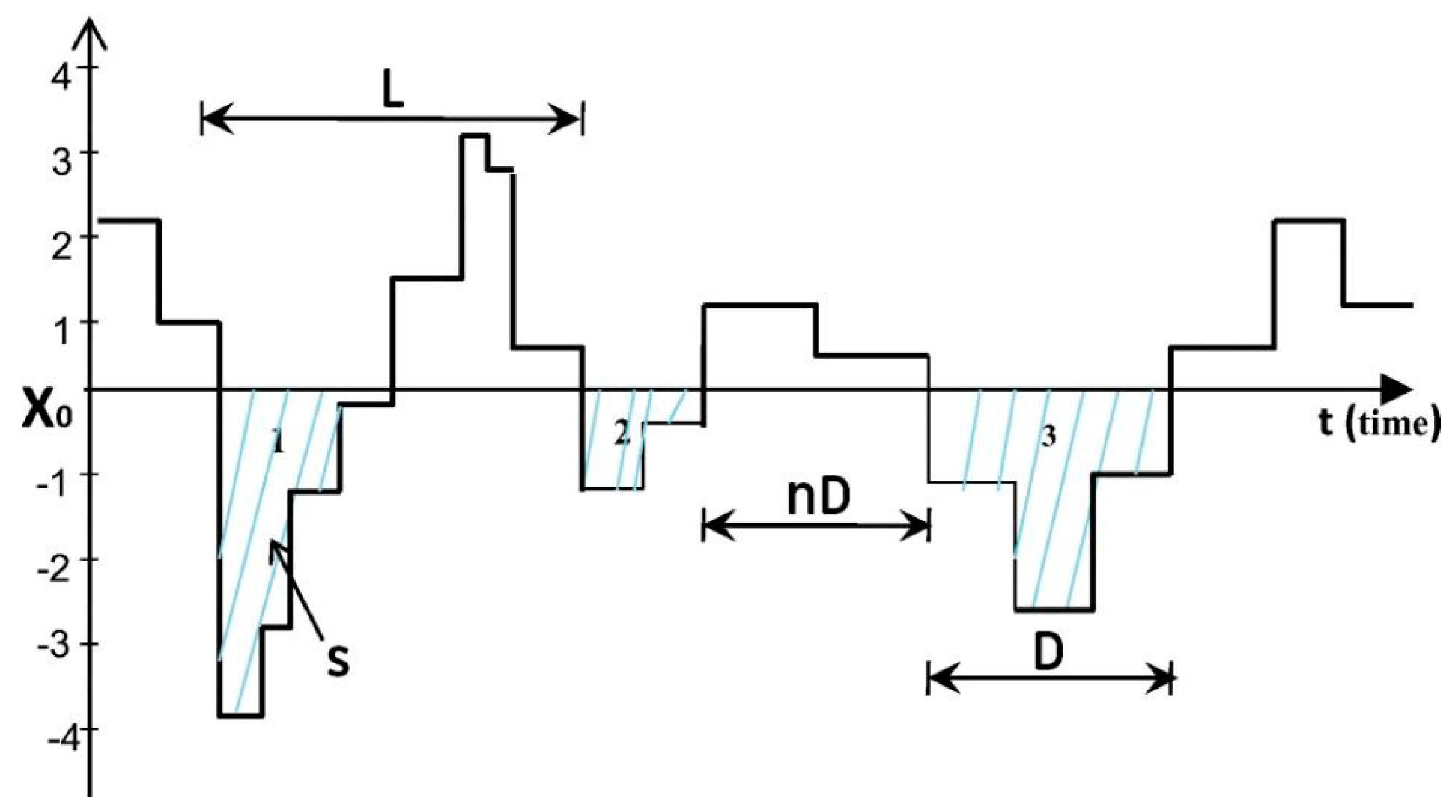
| Drought Level | Setting |
| Weak drought | S = 3 D = 3 |
| Moderate drought | S = 6 D = 6 |
| Strong drought | S = 9 D = 9 |
© 2020 by the authors. Licensee MDPI, Basel, Switzerland. This article is an open access article distributed under the terms and conditions of the Creative Commons Attribution (CC BY) license (http://creativecommons.org/licenses/by/4.0/).
Share and Cite
da Rocha Júnior, R.L.; dos Santos Silva, F.D.; Costa, R.L.; Gomes, H.B.; Pinto, D.D.C.; Herdies, D.L. Bivariate Assessment of Drought Return Periods and Frequency in Brazilian Northeast Using Joint Distribution by Copula Method. Geosciences 2020, 10, 135. https://0-doi-org.brum.beds.ac.uk/10.3390/geosciences10040135
da Rocha Júnior RL, dos Santos Silva FD, Costa RL, Gomes HB, Pinto DDC, Herdies DL. Bivariate Assessment of Drought Return Periods and Frequency in Brazilian Northeast Using Joint Distribution by Copula Method. Geosciences. 2020; 10(4):135. https://0-doi-org.brum.beds.ac.uk/10.3390/geosciences10040135
Chicago/Turabian Styleda Rocha Júnior, Rodrigo Lins, Fabrício Daniel dos Santos Silva, Rafaela Lisboa Costa, Heliofábio Barros Gomes, David Duarte Cavalcante Pinto, and Dirceu Luis Herdies. 2020. "Bivariate Assessment of Drought Return Periods and Frequency in Brazilian Northeast Using Joint Distribution by Copula Method" Geosciences 10, no. 4: 135. https://0-doi-org.brum.beds.ac.uk/10.3390/geosciences10040135