Thematic Maps for the Variation of Bearing Capacity of Soil Using SPTs and MATLAB


Civil Engineering Department, University of Baghdad, 10071 Baghdad, Iraq
*
Author to whom correspondence should be addressed.
Geosciences 2020, 10(9), 329; https://0-doi-org.brum.beds.ac.uk/10.3390/geosciences10090329
Submission received: 4 July 2020
/
Revised: 5 August 2020
/
Accepted: 18 August 2020
/
Published: 20 August 2020
(This article belongs to the Section Geomechanics)
Abstract
:The current study involves placing 135 boreholes drilled to a depth of 10 m below the existing ground level. Three standard penetration tests (SPT) are performed at depths of 1.5, 6, and 9.5 m for each borehole. To produce thematic maps with coordinates and depths for the bearing capacity variation of the soil, a numerical analysis was conducted using MATLAB software. Despite several-order interpolation polynomials being used to estimate the bearing capacity of soil, the first-order polynomial was the best among the other trials due to its simplicity and fast calculations. Additionally, the root mean squared error (RMSE) was almost the same for the all of the tried models. The results of the study can be summarized by the production of thematic maps showing the variation of the bearing capacity of the soil over the whole area of Al-Basrah city correlated with several depths. The bearing capacity of soil obtained from the suggested first-order polynomial matches well with those calculated from the results of SPTs with a deviation of ±30% at a 95% confidence interval.
1. Introduction
Standard penetration test (SPT) is one of the most common and widely used tests in the field around the world. This test considered to be a powerful indicator for the geotechnical properties of soil such as density, shear strength, and compressibility of soils. Additionally, one of the common applications of the SPT is estimation of the liquefaction potential of saturated granular soils for earthquake design. The simplicity, low cost, and global dissemination of SPT equipment and people working on this type of test have led the results of SPTs to be accepted for the preliminary design of foundations [1,2,3,4]. Several corrections can be applied to the measured N-values before using them in the estimation and calculation of the geotechnical properties of soil. The corrected N-value should be representative of the soil medium to give more reliable results. These corrections are suggested by several researches according to their observations to remove the uncertainty of the measure N-values, but the selection of appropriate corrections is important to avoid adding more measured data in the field or calculated in the laboratory. Additionally, the optimization of selected corrections depends mainly on the field conditions of tests, dimensions, and properties of equipment used in tests, diameter, and depth of boreholes. All these conditions should be evaluated by the geotechnical engineer [1,5]. There are several studies correlating the corrected SPT values and different geotechnical properties of soil such density, undrained shear strength, shear wave velocity, and liquefaction potential, but the results of these correlations are still considered preliminary and cannot be used for detailed design of foundations [6,7,8,9,10,11,12,13]. Additionally, the correlation between the results of SPTs with some promising field techniques such as pressuremeter test (PMT) and cone penetration test (CPT) using statistical analysis have been presented, which gives support for the results of SPT by newly developed techniques [14,15,16].
The main objective of this study is to provide thematic maps showing the variation of bearing capacity of soil with geographic coordinates and depth. Several regression analyses were carried out using MATLAB software and the relation between the bearing capacity of the soil and geographic coordinates and depth are being proposed to produce thematic maps. The SPTs were conducted in 135 boreholes (BHs) extended to a depth of 10 m from the existing ground level and distributed over all the plane areas of Al-Basrah city. The soil of this city varies from soft clay to silty clay and sometimes become silty sand, and the results of the study provide a simple and easy tool for calculating the bearing capacity of shallow foundation in Al-Basrah city, which can be used for preliminary design without conducting tests in the field or laboratory [13,17,18,19,20].
2. Standard Penetration Test and Corrections
A standard penetration test (SPT) is one of the recommended field tests for different types of soil when it is difficult to sample and conduct tests in the laboratory. The SPT value (N-value) can be defined as the resistance of the soil to the penetration of a split spoon sample to a distance of 300 mm under constant frequent blows of a standard hammer. Interpretation of SPT results is based on the measured N-value, which is subject to several types of corrections to meet the standard procedure of testing [21,22]. Many factors can affect the measured N-values from SPTs, and these factors can increase or decrease N-value; as a result of such changes in N-values, the calculated geotechnical properties of the soil will be directly affected. Mostly, underestimation of values for geotechnical properties can occur based on correlation equations that depend on SPT values, which leads the results obtained from the SPT to be on the safe side. Accordingly, many corrections can be made to the measured N-values from SPT so that they are reliable, which can lead the geotechnical properties of soil calculated based on correlation with SPT values to be more reliable and widely accepted. The corrections mainly depend on the diameter and depth of the borehole (BH), the type of hammer, the diameter of the rod, and the field conditions, including the confining pressure and the groundwater table (GWT).
Fletcher [23] identified significant causes of error in the SPT and the factors that can affect the measured N-values are:
- Variations from an exact 30 in. drop of the drive weight;
- The use of heavy drill rods of diameter more than 2.5 cm;
- Extreme length of drill rods (over 50 m);
- Interference with free fall of the drive weight from any cause;
- Using a deformed tip on sample spoon;
- Excessive driving of sample spoon before the blow count;
- Failure to seat sampler on undisturbed soil;
Carelessness in counting the blows and measuring penetration.
The necessary corrections that are applied to the measured blow count to obtain the corrected, N1(60) blow count are shown in Equation (1) [24]. The corrected SPT values (N1(60)) are commonly used in empirical correlations to estimate the geotechnical and geophysical properties of soil.
where
N1(60) = corrected SPT value to 60% of the theoretical free-fall hammer energy;
N = measured SPT value (number of blows) in the field;
N’ = N.CW = blow count corrected for groundwater table;
CN = factor of correction for the overburden pressure;
CE = factor of correction for the transmitted energy to the SPT rod;
CW = factor of correction for counting groundwater table;
CB = factor of correction for the diameter of the drilled borehole;
CR = factor of correction for the length of SPT rod;
The rod correction factor (CR) can be taken to be equal to unity for a rod length greater than 6 m [21,22], but Seed et al. [21] recommended CR = 0.75 for a rod length less than 3 m. To avoid complexity, CR is taken to be equal to unity in the present study. Borehole diameter correction should be considered in boreholes of diameter larger than 12 cm, but in the present study the diameter of drilling is 10 cm, so the correction factor (CB) is taken to be equal to unity. Increasing the diameter of the borehole will reduce the measured N-value due to the reduction of confining pressure. It should be noted that many of these factors are not applied in the site investigations. The most widely applied corrections are for overburden stress (CN), groundwater table correction factor (CW), and transmitted energy of the hammer (CE). These three factors will be discussed separately in the next subsections [1,2,3,4,5].
2.1. Groundwater Correction Factor (CW)
Peck et al. [25] proposed a linear interpolation for the correction of groundwater effect on the measured N-values from SPTs. The correction includes a reduction between 50% if the water table is at the ground surface and zero if the groundwater table is encountered at a depth equal to the width of the foundation below the footing, so the suggested correction factor for groundwater table (CW) is:
where is the depth of the groundwater table below the soil surface, is the depth of footing placement, and is the width of the footing. Generally, precautions should be taken to avoid disturbance of the soil bed resulting from the entry of groundwater from the bottom of the borehole and the generation of upward seepage pressure. Another correction can be applied to the measured N-value when the SPT is carried out below the groundwater table, this correction is applied if N is greater than 15, where the resistance of soil increases due to the negative excess porewater pressure generated during the period of SPT [26].
2.2. Overburden Pressure Correction Factor (CN)
Standard penetration tests performed at large depths in a uniform soil deposit will yield higher N-values than shallow tests due to the increased confinement of the overlying soils (vertical effective stresses increase with depth). Therefore, the overburden stress correction normalizes the measured N-value in the field at any depth to a reference stress of 100 kPa. The overburden pressure correction factor recommended by Skempton [22] can be calculated using Equation (4), and this correction is applied to the soil of relative density 40 to 60%.
where is the effective overburden pressure in kPa. At all investigated sites, the soil strata vary from soft clay to silty clay, therefore the saturated and dry unit weight of soil is assumed to be 17 kN/m3 and 15 kN/m3, respectively.
2.3. Energy Correction Factor (CE)
The purpose of the energy correction is to account for tests performed using different types of hammers (e.g., safety, donut, automatic). The safety hammer delivers approximately 60% of the maximum free-fall energy to the drill stem. The donut hammer delivers 45% of the maximum free-fall energy, and the automatic hammer delivers 95% to 100% of the maximum free-fall energy to the drill stem. According to the literature, the energy correction factor (CE) is equal to 0.8–1.0 [22,24,27], but in the present study, it is assumed to be 0.7 to account for the verticality of hammer and the free-fall distance.
3. Study Area and Field Work
The study area is focused on Al-Basrah city, which was established in 636 AD and is located in the southern part of Iraq, with Global Positioning System (GPS) coordinates of 30° 30′ 29.1672″ N and 47° 47′ 0.5604″ E. The area of Al-Basrah city is 181 km2 and it has a population of 2.15 million. It contains the main port of Iraq, Um Qasar, and oil wells. Al-Basrah city is considered an important city globally because of the large oil fields in this city, as well as the Al-Faw port on the Arabian Gulf. The boreholes were drilled to a depth of 10 m below the existing ground level; the average elevation of the ground surface is about 5 m above the sea level. These boreholes were distributed over the whole plane area of the city and were mostly distributed around the two banks of Shatt Al’Arab river, which passes through the city from northwest to southeast. Generally, the quality and level of water play important roles in the variation of allowable bearing capacity of soil.
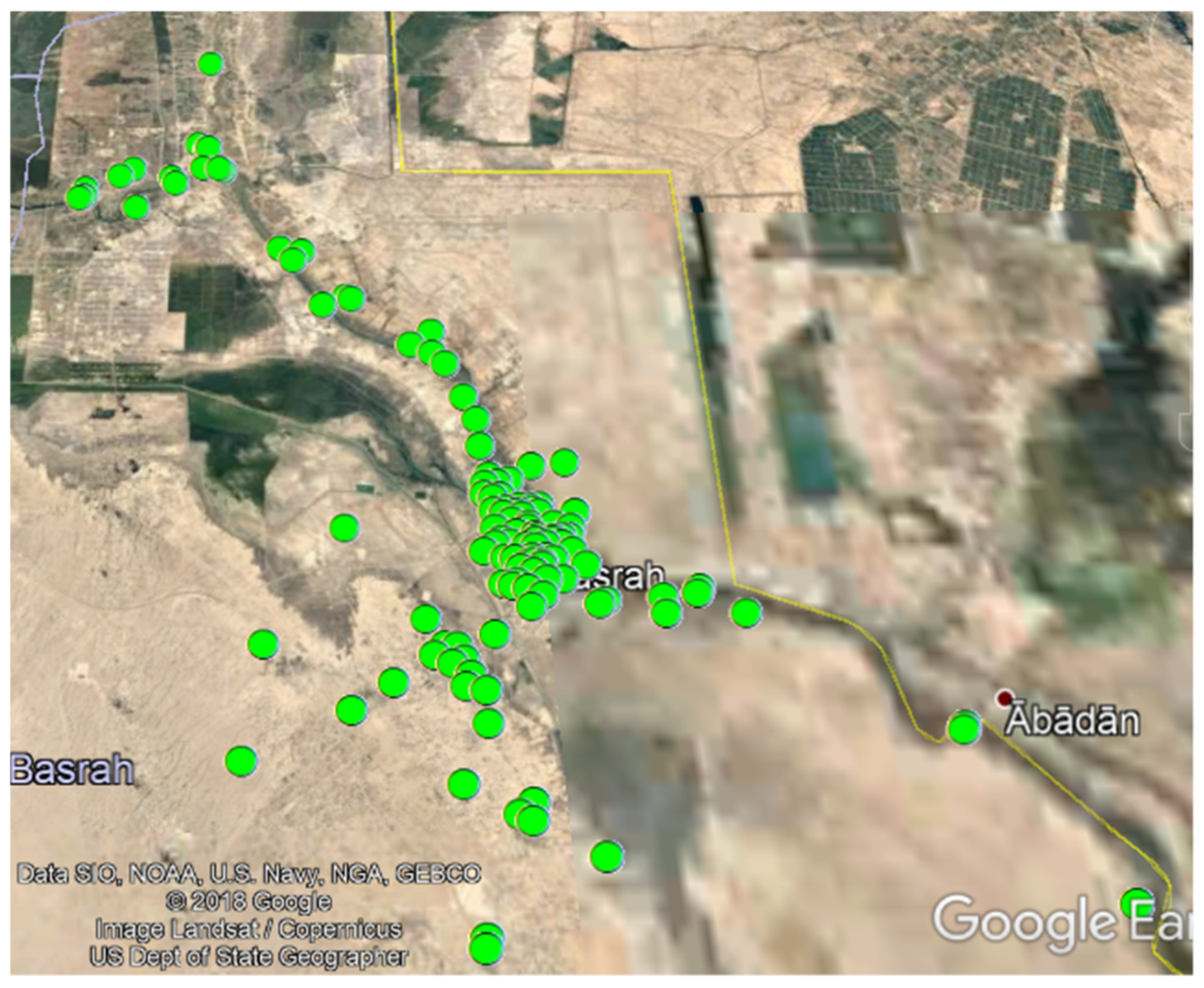
The fieldwork included drilling 135 boreholes distributed arbitrarily over the whole area of Al-Basrah city and mainly located in the available free lots of the city. The drilling of boreholes in free lots is important to avoid problems with the owners of lots and the limited available spaces in the constructed area. Additionally, after selecting the free lots inside the city, the team started locating existing infrastructures such as sewage lines, electricity cables, freshwater pipelines, and telephone and internet cables to avoid any problems during drilling. The boreholes were drilled using a flight auger 10 cm in diameter and extended to a depth of 10 m below the ground surface. Several SPTs were conducted along the depth of boreholes using automatic hammer. In Figure 1, the locations of drilled boreholes are distributed over a satellite image from Google Earth. Additionally, the zone of the surveyed area is shown in Figure 2.
The N-values of SPTs were used to calculate the ultimate bearing capacity of the soil and the soil samples obtained from split spoon samplers were used to calculate the moisture content and specific gravity of the soil. Additionally, the groundwater table was measured in the field after 24 h of drilling and the density of the soil was measured experimentally for each borehole; in some boreholes, the groundwater had not risen after 24 h, so the GWT has no value in Table 1 and does not affect the calculation of the bearing capacity of the soil. These factors are important in the correction of SPT values. The measured N-values from SPTs conducted at depths of 1.5, 6, and 9.5 m below the existing ground surface and GWT for 135 boreholes are given in Table 1. In some boreholes, and at specific depths, such as boreholes 80 and 84 in Table 1, it is difficult to conduct successful SPTs because of the very soft layers of soil at those depths.
4. Bearing Capacity of Soil
Generally, the bearing capacity of soil is considered to be a key to geotechnical engineering, where most of the geotechnical project depends on the bearing capacity of soil. The heterogeneity and layering of soil lead to a high variation in the values of bearing capacity of soil, which requires more effort, time, and cost to conduct reliable soil investigation. Sometimes, the structural loads are small and do not required precise soil investigations, so approximate available equations based on numerical or regression analyses can be used with reliable confidence. Additionally, in most soil investigation reports and for preliminary design purposes, the results of standard penetration tests can be used to evaluate the bearing capacity of soil. This test has an international reputation and is well known in most countries, so this test can be conducted at different depths within drilled boreholes by people with a low level of experience [25,26,28].
The total number of drilled boreholes was 135, but only 95 boreholes were used in this study to avoid the numerical dispersion due to the high difference in the SPT values of some regions adversely affecting the reliability of the results obtained from regression analysis using MATLAB software. The bearing capacity of soil was calculated at depths of 1.5, 6, and 9.5 m for 95 boreholes drilled to a depth of 10 m below the existing ground level and distributed over the whole plane area of Al-Basrah city. The allowable bearing capacity of the soil was calculated based on the results of standard penetration tests conducted at several depths for each borehole after corrections. The heterogeneity of the soil, the high groundwater table, and the high concentrations of organic matter and waste require high value of safety factor to avoid these circumstances, so the safety factor is assumed to be 3 when calculating the allowable bearing capacity of the soil.
The main corrections applied to the measured SPT values in this study are: Overburden Correction Factor (CN), as defined in Equation (4), energy correction factor (CE), which is equal to 0.7, and groundwater correction (CW), as defined in Equations (2) or (3). The bearing capacity of the soil can be calculated based on the corrected N-values. The coordinates of the boreholes and the calculated allowable bearing capacity of soil based on raft footing are given in Table 2. The ultimate bearing capacity of the soil is calculated using Equations (5) to (10), listed below, and the safety factor is equal to 3. The large amount of data used in calculating the ultimate bearing capacity for several depths in 95 boreholes will not be presented in this paper due to the large space required to show such data.
The net ultimate bearing capacity for a raft footing constructed on soil can be calculated from the SPT values using the following equation [29,30].
qult,net is the net ultimate bearing capacity of soil (kN/m2);
B is the width or diameter of foundation (m);
Se is the settlement of soil (mm); in this study, it is assumed equal to 25 mm [30]. Additionally, it is assumed that Df/B = 1, which gives a higher value for Fd and qall.
The allowable bearing capacity of the soil (qall) can be calculated using the following equations.
where
qall is the allowable bearing capacity of soil;
qall,net is the net allowable bearing capacity;
γ′ is the effective unit weight= γsat-γw;
Df is the depth of footing placement;
5. Numerical Modeling of Field Data
The results of SPTs conducted at 135 boreholes were processed by MATLAB to generate a surface expressing the variation of allowable bearing capacity of the soil in the study area. Using the SPT data of 135 boreholes showed high variation and oscillation in the values of the calculated bearing capacity of the soil from MATLAB, so it is important to exclude the extreme data of SPT from calculating the bearing capacity of soil by MATLAB. These extremes may be the result of drilling a small number of boreholes in some locations of the study area, or maybe the high deviation between the bearing capacity of some locations in comparison with the general behavior of the study area. Accordingly, the total number of boreholes used in the analysis by MATLAB is 95 instead of 135 boreholes [31].
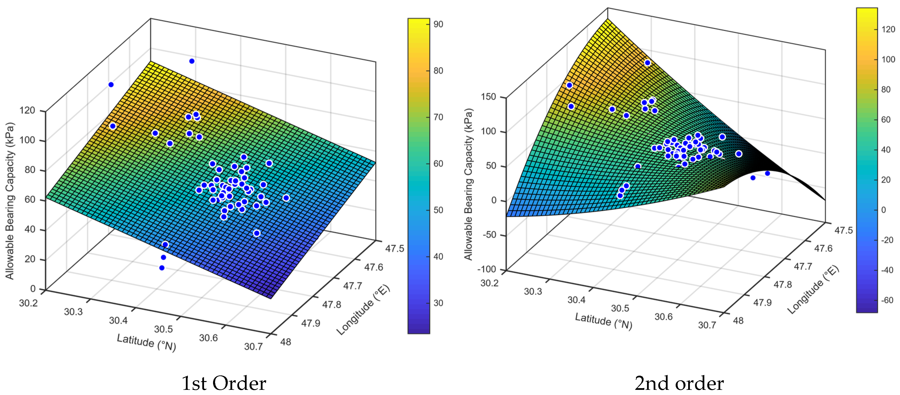
Several trials were conducted to generate an accepted surface representative for the variation of bearing capacity of soil with depth and coordinates using 1st-order surface, 2nd-order surface, 3rd-order surface, and 4th-order surface. The bearing capacity of soil can be calculated from generated surfaces using Equations (12) to (14) and the associated parameters for each equation are given in Table 3 and Table 4. Increasing the order of the polynomial representing the surface of the bearing capacity of soil will generate a more accurate surface, but the complexity will increase by increasing the number of parameters required to calculate the bearing capacity of the soil. It is noticed that increasing the order of the surface polynomial from first to fourth increases the number of parameters from 3 to 15, while the root mean squared error (RMSE) did not increase significantly, as shown in Table 3. The generated surfaces for variation of bearing capacity at a depth of 1.5 m for 95 boreholes using 1st-, 2nd-, 3rd-, and 4th-order polynomials are shown in Figure 3 and Figure 4.
The first- and second-order interpolation polynomials almost generate plane surfaces; these surfaces simply express the variation of allowable bearing capacity with coordinates and depth. Additionally, it is easy to use the equation with a smaller number of parameters, but using third- and fourth-order interpolations will generate surfaces with complex folds that produce very sensitive estimation for the allowable bearing capacity of soil, especially at the inflection point of surfaces. Accordingly, it is recommended using 1st-order interpolation, where the polynomial of the surface has only three parameters and an acceptable root mean squared error (RMSE) in comparison with other suggested surfaces to reduce effort and time required for estimation the allowable bearing capacity of the soil. Additionally, R2 is the proportion of the variance in the dependent variable that is predictable from the independent variable(s), and this factor varies from 0.1544 to 0.3539 for the data used in this study. The value of R2 increased with the increase in the order of polynomial used in modeling of experimental data, which reflected a greater convergence between predicated values of allowable bearing capacity of soil and those measured experimentally from SPTs. The adjusted R-squared is a modified version of R-squared that has been adjusted for the number of predictors in the model.
First-order model (with 95% confidence bounds) is:
Second-order model (with 95% confidence bounds) is:
Third-order model (with 95% confidence bounds) is:
Fourth-order model (with 95% confidence bounds) is:
where x and y are the geographic coordinates of the point.
6. Results and Discussion
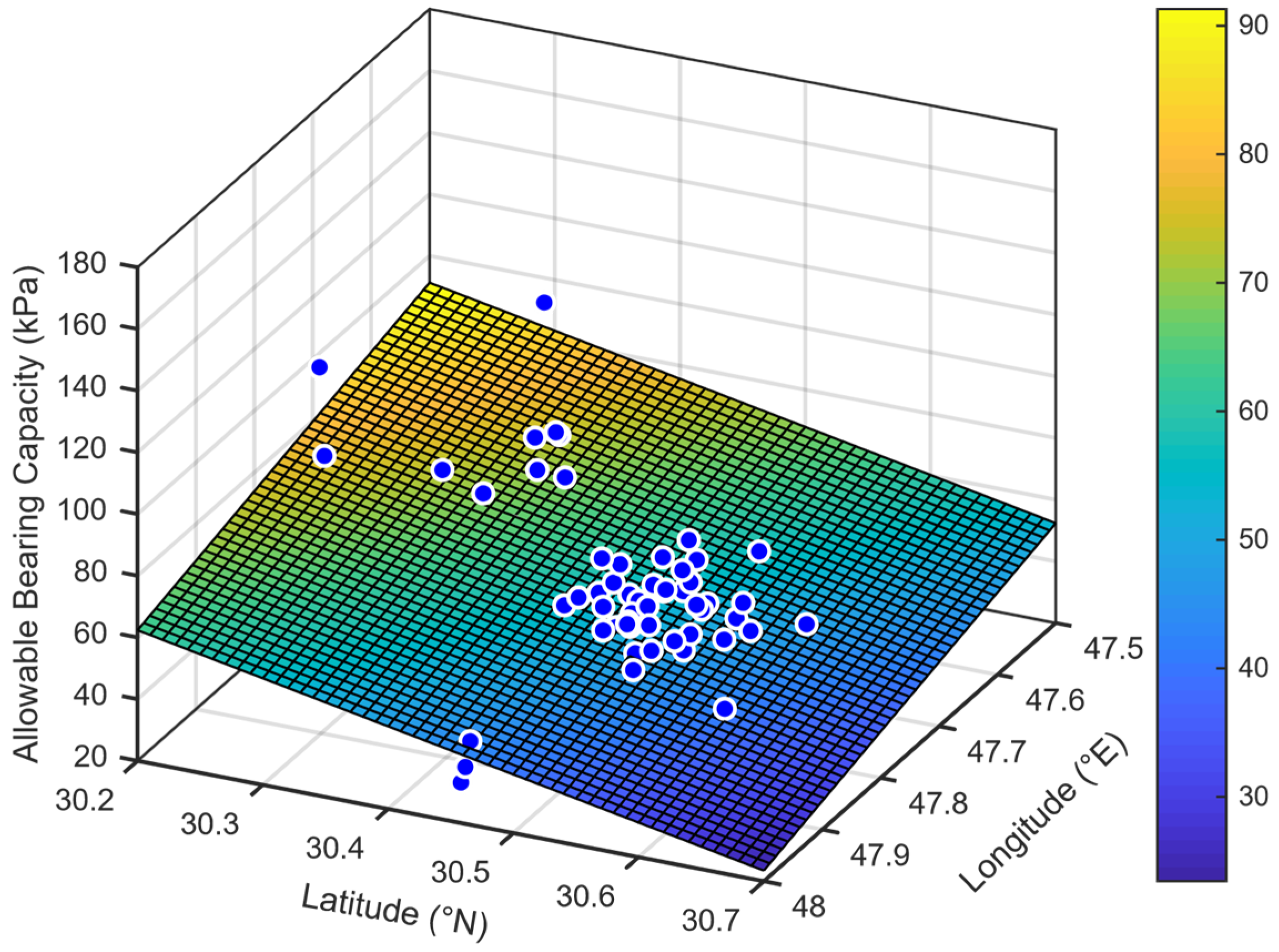
The first-order interpolation presented in the previous section will be used to estimate the allowable bearing capacity of soil at depths 1.5, 6, and 9.5 m depending on the coordinates of 95 boreholes and the corrected N-values obtained from SPTs. The equation of the surface generated from the first-order interpolation will be the same for the investigated depths as defined in Equation (11), but with different values for parameters defining this equation for each depth. The values of these parameters are given in Table 5. The values of the parameters showed high nonhomogeneity due to the high variation of measured SPT values [32].
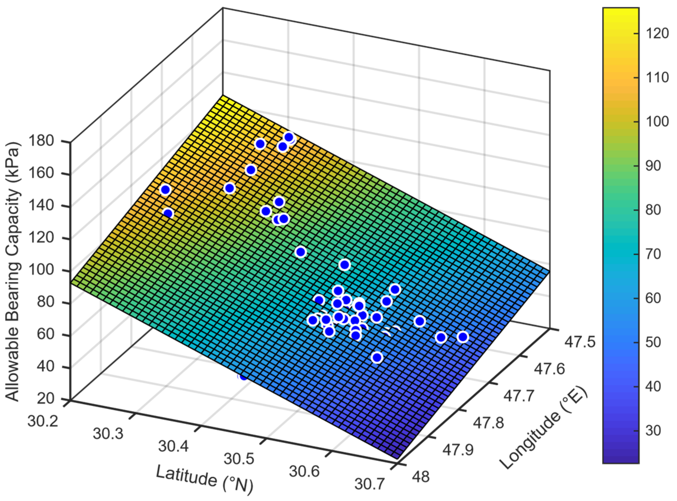
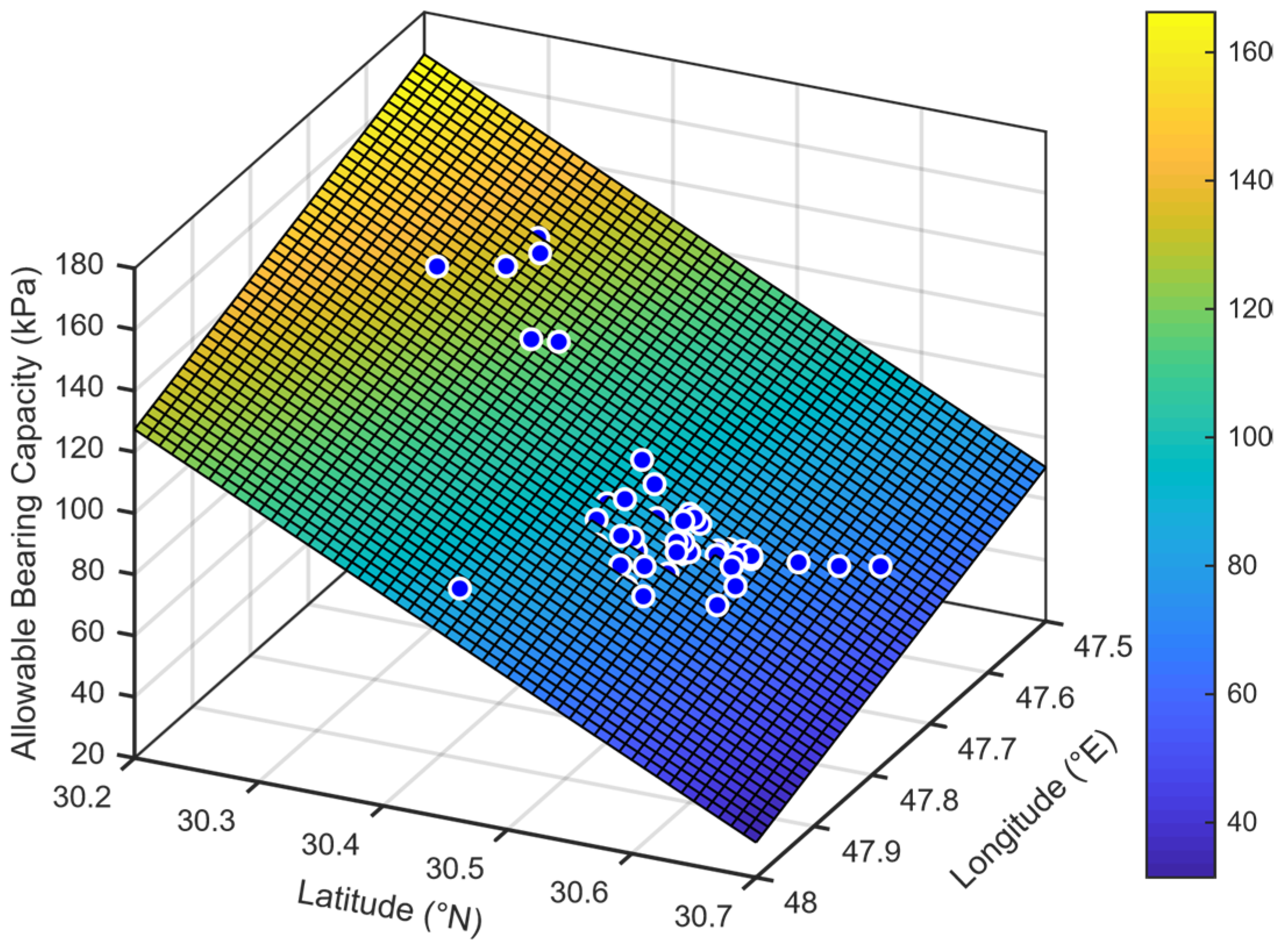
Mostly, the SPT values decreased with depth, which reflects layers of well-compacted soil at the surface and layers of soft soils after 1.5 m depth, but the soil acquired its strength from the overburden pressure. In this study, the overburden pressure is calculated based on the effective unit weight to avoid the uncertainty coming from SPT values and seasonal variation of the GWT. The surfaces showing the variation of allowable bearing capacity are planes because the equation of first-order interpolation is linear, as shown in Figure 5, Figure 6 and Figure 7. The variation showed that the allowable bearing capacity of soil in the northern parts of city is higher than that in the southern parts. Additionally, the allowable bearing capacity of soil increases with increasing depth. The same trend was noted for the three studied depths. The weak zone, according to the allowable bearing capacity, is in the southeast part of the city, where the bearing capacity of the soil is mostly less than 4 kPa.
where x is equal to E − 47.5 and y is equal to N − 30.2; E is easting (longitude) in degrees and N is northing (latitude) in degrees.
Generally, it is important to evaluate the accuracy of suggested surfaces to estimate the allowable bearing capacity, so the estimated values of qall are compared with those calculated from SPTs. The results showed a good agreement between both estimated and calculated values of qall at several depths, where the difference between the maximum and minimum values of qall ranged (−31.52 to 88.36)%, (−30.77 to −12.53)%, and (−33.13 to −23.36)% at depths of 1.5, 6, and 9.5 m respectively as shown in Table 6. In most cases, the numerical model gives values for qall lower than that calculated from the results of SPTs as underestimation. Therefore, the suggested numerical model can be used safely with an accepted under estimation values for qall by 30%.
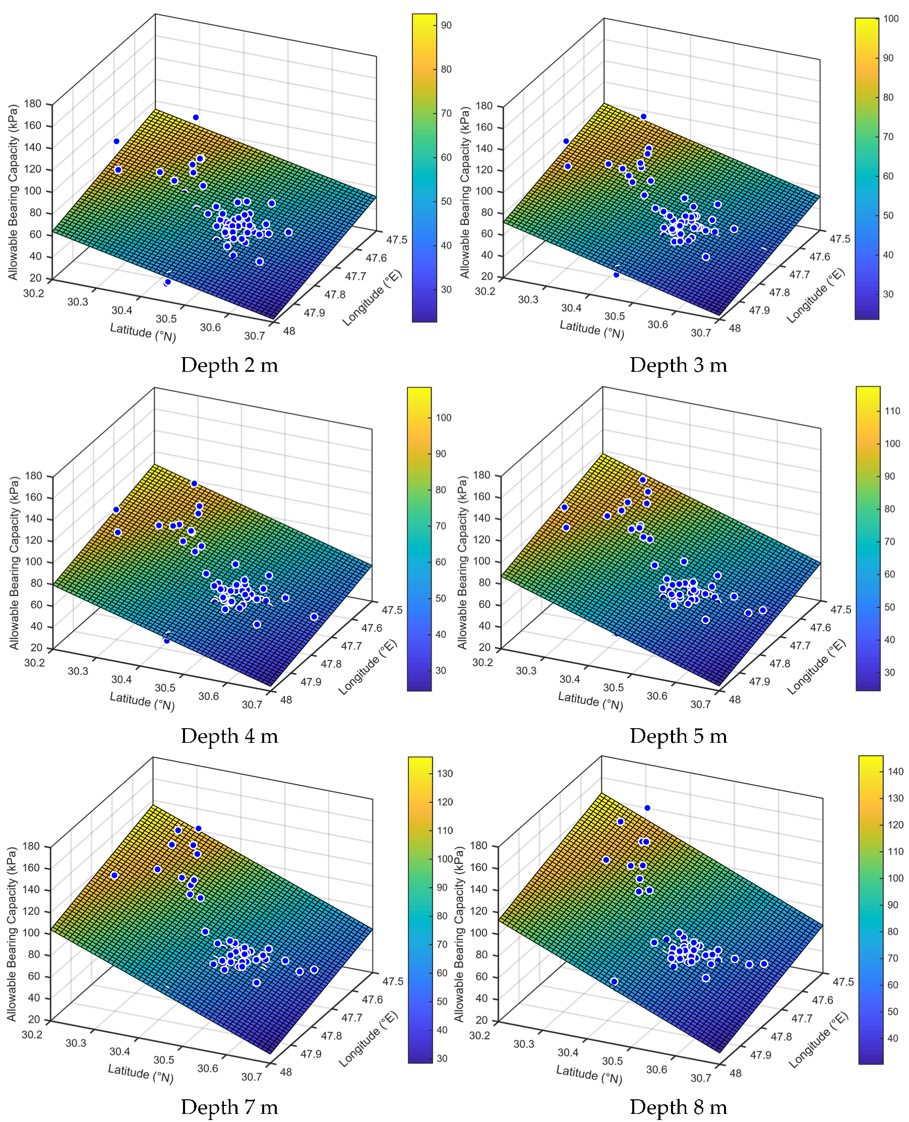
The suggested numerical model can be extended to estimate the allowable bearing capacity of the soil at depths of 2, 3, 4, 5, 7, and 8 m from the ground surface. A linear interpolation was used to find the corresponding corrected SPT values at these depths. Based on the calculated SPT values, the first-order numerical model is used to draw a surface for the variation of qall with coordinates and depths. The parameters of the suggested first-order numerical model are given in Table 7 and the variation of qall with coordinates and depths (2, 3, and 4 m) are shown in Figure 8. The same trend in variation of qall is noticed, where the maximum values of qall are at the north and start to decrees towards the south especially the southeast.
7. Conclusions
The present work includes a whole soil survey for Al-Basrah city, which is an important city in Iraq. The soil survey included drilling of 135 boreholes to a depth of 10 m below the existing ground level. For each borehole, three SPT tests were carried out at depths of 1.5, 6, and 9.5 m, and the measured N-values from SPT were subjected to some important corrections. The corrected N-values were used to calculate the allowable bearing capacity of the soil. One of the important parts of soil investigation is the preliminary investigation, which provides a general conception of the variation in the allowable bearing capacity of soil over the whole plane area of Al-Basrah city, and the resulting soil parameters from the preliminary investigation can be used in the preliminary design of foundations. Additionally, one of the promising techniques is to use numerical analysis to build a 3-D surface that shows the variation of allowable bearing capacity of soil with coordinates and depth. Several models were used to calculate the allowable bearing capacity of soil, but the simplest and easiest one was the first-order polynomial, which depends on three parameters only and gives an RMSE of 19.3404. The results of the suggested numerical model showed good agreement with those calculated from the SPT results, and the numerical model underestimated the results of allowable bearing capacity of soil by almost 30% with respect to the measured values from SPT. Additionally, using the results of the present numerical model will help to save time and money especially for low-cost projects.
Author Contributions
Conceptualization, M.O.K. and M.D.A.; methodology, M.O.K.; software, A.A.-R.; validation, M.O.K., M.D.A. and A.A-H.S.; formal analysis, M.O.K.; investigation, M.O.K.; resources, M.D.A.; data curation, A.A.-R.; writing—original draft preparation, M.O.K.; writing—review and editing, A.A.-H.S. and A.A.-R.; visualization, M.D.A.; supervision, M.O.K.; project administration, M.O.K.; funding acquisition, M.D.A., A.A.-H.S., and A.A.-R. All authors have read and agreed to the published version of the manuscript.
Funding
This research received no external funding
Acknowledgments
The authors express their appreciation to the staff of the Consultative Bureau at the College of Sciences/University of Babylon for their support in providing the necessary data.
Conflicts of Interest
The authors declare no conflict of interest.
References
- Clayton, C.R.I.; Matthews, M.C.; Simons, N.E. Site Investigation, 2nd ed.; Blackwell Science: London, UK, 1995. [Google Scholar]
- Rocha, B.P.; Giacheti, H.L. Site characterization of a tropical soil by in situ tests. Dyna 2018, 85, 211–219. [Google Scholar] [CrossRef]
- McGregor, J.A.; Duncan, J.M. Performance and Use of the Standard Penetration Test in Geotechnical Engineering Practice; Center for Geotechnical Practice and Research, Virginia Tech; Virginia Polytechnic Institute and State University: Blacksburg, VA, USA, 1998. [Google Scholar]
- Decourt, L. Standard Penetration Test State-of-the-Art-Report; Norwegian Geotechnical Institute: Oslo, Norway, 1990. [Google Scholar]
- Page, M.; Bradshaw, A.S.; Mike Sherrill, P.E. Guidelines for Geotechnical Site Investigations in Rhode Island Final Report; University of Rhode Island: Narragansett, RI, USA, 2005. [Google Scholar]
- Ghafghazi, M.; DeJong, J.T.; Sturm, A.P.; Temple, C.E. Instrumented Becker penetration test. II: iBPT-SPT correlation for characterization and liquefaction assessment of gravelly soils. J. Geotech. Geoenviron. Eng. 2017, 143, 04017063. [Google Scholar] [CrossRef] [Green Version]
- Bahmani, S.M.; Briaud, J.L. Modulus to SPT Blow Count Correlation for Settlement of Footings on Sand. In Geo-Congress 2020: Foundations, Soil Improvement, and Erosion 2020; American Society of Civil Engineers: Reston, VA, USA, 2020; pp. 343–349. [Google Scholar]
- Kirar, B.; Maheshwari, B.K.; Muley, P. Correlation between shear wave velocity (Vs) and SPT resistance (N) for Roorkee region. Int. J. Geosynth. Gr. Eng. 2016, 2, 9. [Google Scholar] [CrossRef] [Green Version]
- Rahimi, S.; Wood, C.M.; Wotherspoon, L.M. Influence of soil aging on SPT-Vs correlation and seismic site classification. Eng. Geol. 2020, 272, 105653. [Google Scholar] [CrossRef]
- Anbazhagan, P.; Uday, A.; Moustafa, S.S.; Al-Arifi, N.S. Correlation of densities with shear wave velocities and SPT N values. J. Geophys. Eng. 2016, 13, 320–341. [Google Scholar] [CrossRef] [Green Version]
- Bandyopadhyay, S.; Sengupta, A.; Reddy, G.R. Development of correlation between SPT-N value and shear wave velocity and estimation of non-linear seismic site effects for soft deposits in Kolkata city. Geomech. Geoengin. 2019, 1–19. [Google Scholar] [CrossRef]
- Thokchom, S.; Rastogi, B.K.; Dogra, N.N.; Pancholi, V.; Sairam, B.; Bhattacharya, F.; Patel, V. Empirical correlation of SPT blow counts versus shear wave velocity for different types of soils in Dholera, Western India. Nat. Hazards 2017, 86, 1291–1306. [Google Scholar] [CrossRef]
- Mujtaba, H.; Farooq, K.; Sivakugan, N.; Das, B.M. Evaluation of relative density and friction angle based on SPT-N values. KSCE J. Civ. Eng. 2018, 22, 572–581. [Google Scholar] [CrossRef]
- Liang, X.; Qin, Z.; Chen, S.; Wang, D. CPT-SPT correlation analysis based on BP artificial neural network associated with partial least square regression. In Proceedings of the GeoShanghai 2018 International Conference: Multi-physics Processes in Soil Mechanics and Advances in Geotechnical Testing, Shanghai, China, 27–30 May 2018; pp. 381–390. [Google Scholar] [CrossRef]
- Anwar, M.B. Correlation between PMT and SPT results for calcareous soil. HBRC J. 2018, 14, 50–55. [Google Scholar] [CrossRef]
- Balachandran, K.; Liu, J.; Cao, L.; Peaker, S. Statistical Correlations between Pressuremeter Tests and SPT for Glacial Tills. In Proceedings of the 4th Geo-China International Conference, Shandong, China, 25–27 July 2016; pp. 133–140. [Google Scholar] [CrossRef]
- Eldeen Taha, O.M. Variation of bearing capacity prediction for shallow foundations by SPT and laboratory tests. Int. J. GEOMATE 2019, 17, 108–114. [Google Scholar] [CrossRef]
- Singh, N.B.; Jibanchand, N.; Devi, K.R. Applicability of standard penetration tests to estimate undrained shear strength of soils of Imphal. Int. J. Eng. Technol. Sci. Res. 2017, 4, 250–255. [Google Scholar]
- Heidarie Golafzani, S.; Jamshidi Chenari, R.; Eslami, A. Reliability based assessment of axial pile bearing capacity: Static analysis, SPT and CPT-based methods. Georisk Assess. Manag. Risk Eng. Syst. Geohazards 2019, 1–15. [Google Scholar] [CrossRef]
- Ferreira, M.; Tsuha, C.; Schiavon, J.; Aoki, N. Determination of SPT end bearing and side friction resistances using static uplift tests. Geotech. Test. J. 2016, 39, 1040–1047. [Google Scholar] [CrossRef]
- Seed, H.B.; Tokimatsu, K.; Harder, L.F.; Chung, R.M. The Influence of SPT Procedures in Soil Liquefaction Resistance Evaluations; Report No. UCB/EERC84/15 Earthquake Engineering Research Center; University of California: Berkeley, CA, USA, 1984. [Google Scholar]
- Skempton, A.W. Standard penetration test procedures and the effects in sands of overburden pressure, relative density, particle size, aging and overconsolidation. Geotechnique 1986, 36, 425–447. [Google Scholar] [CrossRef]
- Fletcher, G.F.A. Standard Penetration Test: Its uses and abuses. ASCE J. Geotech. Eng. 1985, 91, 67–75. [Google Scholar]
- Youd, T.L.; Idriss, I.M. Liquefaction resistance of soils: Summary report from the 1996 NCEER and 1998 NCEER/NSF workshops on evaluation of liquefaction resistance of soils. J. Geotech. Geoenviron. Eng. 2001, 127, 297–313. [Google Scholar] [CrossRef] [Green Version]
- Peck, R.B.; Hanson, W.E.; Thornburn, T.H. Foundation Engineering; John Wiley & Sons: New York, NY, USA, 1974. [Google Scholar]
- Craig, R.F. Craig’s Soil Mechanics; Spon, Taylor & Francis Group: New York, NY, USA, 2004. [Google Scholar]
- Matsumoto, T.; Phan, L.T.; Oshima, A.; Shimono, S. Measurements of driving energy in SPT and various dynamic cone penetration tests. Soils Found. 2015, 55, 201–212. [Google Scholar] [CrossRef] [Green Version]
- Carter, M.; Bentley, S.P. Soil Properties and their Correlations; John Wiley & Sons: Chichester, UK, 2016. [Google Scholar]
- Bowles, J. Foundation Analysis and Design; McGraw-Hill: New York, NY, USA, 1998. [Google Scholar]
- Das, B.M. Principles of Foundation Engineering; Cengage Learning: Boston, MA, USA, 2015. [Google Scholar]
- Kulhawy, F.H.; Trautman, C.H. Estimation of in-situ uncertainty. In Uncertainty in the Geologic Environment; ASCE GSP: New York, NY, USA, 1996; pp. 269–286. [Google Scholar]
- Schnaid, F.; Lourenço, D.; Odebrecht, E. Interpretation of static and dynamic penetration tests in coarse-grained soils. Géotech. Lett. 2017, 7, 113–118. [Google Scholar] [CrossRef]
Figure 1.
Locations of the boreholes on Google map.

Figure 2.
Locations of boreholes used in the analysis.

Figure 3.
Variation of the allowable bearing capacity of soil at 1.5 m depth using 1st- and 2nd-order interpolation.
Figure 3.
Variation of the allowable bearing capacity of soil at 1.5 m depth using 1st- and 2nd-order interpolation.

Figure 4.
Variation of the allowable bearing capacity of soil at 1.5 m depth using 3rd and 4th-order interpolation.
Figure 4.
Variation of the allowable bearing capacity of soil at 1.5 m depth using 3rd and 4th-order interpolation.

Figure 5.
Variation of the allowable bearing capacity of soil at 1.5 m depth.

Figure 6.
Variation of the allowable bearing capacity of soil at 6 m depth.

Figure 7.
Variation of the allowable bearing capacity of soil at 9.5 m depth.

Figure 8.
Variation of the allowable bearing capacity of soil at depths 2, 3, 4, 5, 7, and 8 m.


Table 1.
Measured N-value of drilled boreholes and allowable bearing capacity of soil calculated based on corrected N-values of SPTs.
Table 1.
Measured N-value of drilled boreholes and allowable bearing capacity of soil calculated based on corrected N-values of SPTs.
| BH (No.) | GPS Coordinates | GWT (m) | N-Value | BH (No.) | GPS Coordinates | GWT (m) | N-Value | ||||||
|---|---|---|---|---|---|---|---|---|---|---|---|---|---|
| Latitude Degree | Longitude Degree | 1.5 m | 6.0 m | 9.5 m | Latitude Degree | Longitude Degree | 1.5 m | 6.0 m | 9.5 m | ||||
| 1 | 30.46324 | 47.764810 | 1.2 | 2 | 2 | 2 | 69 | 30.984759 | 47.332300 | 0.9 | 2 | 2 | 2 |
| 2 | 30.677667 | 47.737333 | 0.5 | 3 | 2 | 2 | 70 | 30.457774 | 47.983043 | 0.5 | 5 | 2 | 2 |
| 3 | 30.353224 | 47.736546 | 1.0 | 10 | 20 | 50 | 71 | 30.945994 | 47.270258 | 1.0 | 6 | 2 | 2 |
| 4 | 30.866987 | 47.548848 | 1.0 | 7 | 2 | 2 | 72 | 30.357404 | 47.715029 | 1.0 | 6 | 25 | 50 |
| 5 | 30.943651 | 47.263842 | 2.25 | 7 | 2 | 2 | 73 | 30.985692 | 47.422968 | 1.0 | 2 | 2 | 2 |
| 6 | 30.498979 | 47.846098 | 1.25 | 23 | 5 | 2 | 74 | 30.513353 | 47.819846 | 1.0 | 10 | 2 | 2 |
| 7 | 30.452369 | 47.979893 | 2.1 | 4 | 2 | 6 | 75 | 30.532567 | 47.780909 | 1.2 | 8 | 2 | 2 |
| 8 | 30.384517 | 47.715239 | - | 41 | 33 | 28 | 76 | 30.32028 | 47.735860 | - | 23 | 29 | 34 |
| 9 | 30.65027 | 47.750105 | 0.25 | 2 | 2 | 2 | 77 | 30.42647 | 47.675920 | - | 19 | 16 | 10 |
| 10 | 30.97454 | 47.315320 | 2.0 | 10 | 7 | 2 | 78 | 30.36121 | 47.637050 | 1.0 | 22 | 26 | 40 |
| 11 | 31.01347 | 47.427324 | 1.5 | 10 | 8 | 2 | 79 | 30.46789 | 47.832280 | 2.0 | 3 | 3 | 2 |
| 12 | 30.929563 | 47.337608 | 1.0 | 2 | 2 | 2 | 80 | 30.52529 | 47.590030 | 0.5 | - | - | 6 |
| 13 | 30.618512 | 47.751902 | 3.0 | 8 | 4 | 2 | 81 | 30.743122 | 47.6781175 | 2.0 | 2 | 2 | 2 |
| 14 | 30.802983 | 47.608714 | 2.0 | 7 | 2 | 2 | 82 | 30.05258 | 47.925830 | 0.5 | 2 | 2 | 2 |
| 15 | 30.5068 | 47.835369 | 1.2 | 4 | 2 | 2 | 83 | 30.24478 | 47.776060 | - | 31 | 29 | 27 |
| 16 | 30.492526 | 47.815992 | 0.5 | 4 | 4 | 2 | 84 | 30.40101 | 47.496740 | 0.5 | - | 41 | 43 |
| 17 | 30.561206 | 47.770233 | 0.75 | 6 | 4 | 2 | 85 | 30.575532 | 47.768340 | 1.5 | 2 | 2 | 2 |
| 18 | 30.511275 | 47.824614 | 2.0 | 8 | 4 | 2 | 86 | 30.04477 | 47.918890 | 1.5 | 2 | 2 | 2 |
| 19 | 30.549429 | 47.813952 | 1.2 | 3 | 3 | 4 | 87 | 30.19468 | 47.845510 | - | 15 | 24 | 34 |
| 20 | 30.519017 | 47.784783 | 1.0 | 10 | 10 | 2 | 88 | 30.49137 | 47.769600 | 1.5 | 8 | 4 | 2 |
| 21 | 30.503642 | 47.805022 | 1.95 | 8 | 3 | 7 | 89 | 30.43096 | 48.030270 | 2.5 | 2 | 2 | 2 |
| 22 | 30.5143 | 47.844199 | 1.2 | 2 | 2 | 2 | 90 | 29.582635 | 48.273090 | 1.25 | 2 | 2 | 2 |
| 23 | 30.451235 | 47.808062 | 0.25 | 7 | 3 | 3 | 91 | 30.487565 | 47.802265 | 1.5 | 8 | 2 | 3 |
| 24 | 30.476148 | 47.80068 | 1.25 | 6 | 2 | 3 | 92 | 30.43907 | 47.793667 | 0.5 | 3 | 2 | 3 |
| 25 | 30.398134 | 47.708611 | 1.5 | 14 | 18 | 35 | 93 | 30.498611 | 47.746389 | 0.5 | 2 | 2 | 2 |
| 26 | 30.524343 | 47.761026 | 1.5 | 8 | 4 | 3 | 94 | 30.558264 | 47.761877 | 0.5 | 2 | 2 | 2 |
| 27 | 30.542873 | 47.791312 | 1.5 | 12 | 6 | 3 | 95 | 30.410137 | 47.750771 | - | 11 | 19 | 30 |
| 28 | 30.545661 | 47.775351 | 2.1 | 8 | 2 | 5 | 96 | 30.548722 | 47.790806 | 0.75 | 8 | 3 | 3 |
| 29 | 30.528592 | 47.800295 | 0.8 | 9 | 6 | 3 | 97 | 30.483453 | 47.810493 | 1.5 | 8 | 2 | 5 |
| 30 | 30.444847 | 47.876889 | 1.2 | 2 | 2 | 2 | 98 | 30.511952 | 47.767686 | 1.5 | 8 | 4 | 4 |
| 31 | 30.562611 | 47.752161 | 1.8 | 7 | 2 | 2 | 99 | 30.514264 | 47.835641 | 1.2 | 8 | 5 | 3 |
| 32 | 30.46125 | 47.775306 | 1.0 | 6 | 2 | 3 | 100 | 30.504509 | 47.795087 | 0.95 | 8 | 2 | 2 |
| 33 | 30.492161 | 47.800100 | 1.4 | 10 | 4 | 3 | 101 | 30.468246 | 47.820135 | 2.1 | 18 | 13 | 2 |
| 34 | 30.528288 | 47.828266 | 1.25 | 8 | 7 | 11 | 102 | 30.380307 | 47.702145 | 10.0 | 34 | 38 | 35 |
| 35 | 30.542023 | 47.853618 | 0.25 | 7 | 6 | 4 | 103 | 30.759306 | 47.704500 | 0.25 | 6 | 2 | 2 |
| 36 | 30.490531 | 47.780647 | 1.63 | 8 | 4 | 4 | 104 | 30.261936 | 47.704736 | - | 9 | 10 | 17 |
| 37 | 30.574453 | 47.753307 | 0.5 | 6 | 2 | 2 | 105 | 30.485403 | 47.811495 | 1.0 | 4 | 3 | 2 |
| 38 | 30.388941 | 47.683118 | 1.0 | 12 | 25 | 50 | 106 | 30.467966 | 47.813826 | 0.6 | 4 | 4 | 2 |
| 39 | 30.5079 | 47.777086 | 0.5 | 8 | 3 | 3 | 107 | 30.465589 | 47.780119 | 2.1 | 8 | 3 | 3 |
| 40 | 30.369006 | 47.721302 | 10.0 | 13 | 18 | 26 | 108 | 30.28501 | 47.472570 | 1.2 | 8 | 2 | 3 |
| 41 | 30.448513 | 47.941167 | 3.5 | 5 | 2 | 2 | 109 | 30.543719 | 47.761162 | 2.2 | 8 | 3 | 4 |
| 42 | 30.516736 | 47.805846 | 0.9 | 8 | 2 | 3 | 110 | 30.315603 | 48.242598 | 2.5 | 2 | 2 | 2 |
| 43 | 30.79525 | 47.573028 | 0.25 | 2 | 2 | 2 | 111 | 30.541672 | 47.785828 | 0.7 | 9 | 6 | 5 |
| 44 | 30.545003 | 47.804686 | 0.5 | 6 | 3 | 4 | 112 | 30.538565 | 47.793098 | 1.0 | 10 | 4 | 2 |
| 45 | 30.123251 | 47.717260 | - | 50 | 45 | 42 | 113 | 30.548753 | 47.800998 | 1.1 | 7 | 6 | 4 |
| 46 | 30.506425 | 47.759875 | 0.5 | 4 | 4 | 6 | 114 | 30.524387 | 47.798975 | 1.1 | 4 | 4 | 2 |
| 47 | 29.973944 | 48.468417 | - | 2 | 2 | 2 | 115 | 30.578647 | 47.781908 | 1.0 | 2 | 2 | 2 |
| 48 | 30.719042 | 47.718392 | 1.25 | 6 | 2 | 2 | 116 | 30.524472 | 47.847061 | 1.0 | 6 | 4 | 2 |
| 49 | 30.594667 | 47.809473 | 2.1 | 10 | 8 | 2 | 117 | 30.114687 | 47.715509 | - | 50 | 48 | 46 |
| 50 | 30.458433 | 47.791947 | 1.2 | 4 | 2 | 4 | 118 | 30.233761 | 47.760731 | 1.0 | 46 | 40 | 35 |
| 51 | 30.98478 | 47.443770 | 1.0 | 8 | 7 | 2 | 119 | 29.971258 | 48.476035 | 1.0 | 2 | 2 | 2 |
| 52 | 30.489653 | 47.823968 | 3.0 | 8 | 3 | 4 | 120 | 30.44163 | 47.869875 | 2.2 | 6 | 2 | 2 |
| 53 | 30.483358 | 47.859833 | 2.1 | 2 | 2 | 2 | 121 | 30.732536 | 47.703688 | 1.25 | 6 | 2 | 2 |
| 54 | 30.399438 | 47.695805 | - | 33 | 22 | 35 | 122 | 30.805461 | 47.601909 | 2.0 | 6 | 2 | 2 |
| 55 | 30.33382 | 47.590580 | - | 50 | 45 | 42 | 123 | 30.855089 | 47.53756 | 2.0 | 2 | 2 | 2 |
| 56 | 30.506131 | 47.816672 | 2.1 | 8 | 2 | 5 | 124 | 30.981152 | 47.449086 | 0.25 | 7 | 2 | 2 |
| 57 | 30.3117 | 48.240450 | 1.5 | 2 | 2 | 2 | 125 | 30.971853 | 47.382546 | 0.25 | 2 | 2 | 2 |
| 58 | 31.020338 | 47.416235 | 1.0 | 8 | 2 | 2 | 126 | 30.956501 | 47.271284 | 0.25 | 4 | 2 | 2 |
| 59 | 30.431172 | 47.942036 | 4.0 | 2 | 2 | 2 | 127 | 31.015355 | 47.429864 | 0.5 | 8 | 2 | 6 |
| 60 | 30.583858 | 47.758782 | 3.2 | 12 | 8 | 2 | 128 | 31.144262 | 47.43092 | 2.5 | 2 | 7 | 2 |
| 61 | 30.032503 | 47.919989 | 2.5 | 19 | 23 | 14 | 129 | 30.149344 | 48.373275 | 1.0 | 2 | 2 | 2 |
| 62 | 30.22773 | 47.773719 | - | 29 | 25 | 30 | 130 | 30.513148 | 47.82633 | 1.25 | 4 | 2 | 2 |
| 63 | 30.963884 | 47.387458 | 2.6 | 10 | 2 | 2 | 131 | 30.541316 | 47.812604 | 1.5 | 7 | 2 | 2 |
| 64 | 30.541292 | 47.854056 | 2.1 | 5 | 10 | 2 | 132 | 30.510489 | 47.805907 | 2.0 | 3 | 2 | 4 |
| 65 | 30.540332 | 47.772309 | 1.2 | 10 | 4 | 5 | 133 | 30.5145 | 47.80936 | 0.5 | 3 | 3 | 3 |
| 66 | 30.870981 | 47.521570 | 1.25 | 2 | 2 | 2 | 134 | 30.598381 | 47.848881 | 1.0 | 5 | 2 | 2 |
| 67 | 30.583779 | 47.758780 | 1.25 | 5 | 2 | 2 | 135 | 30.487600 | 47.798300 | 2.1 | 14 | 3 | 2 |
| 68 | 30.480276 | 47.785883 | 0.5 | 8 | 5 | 5 | - | - | - | - | - | - | - |
Table 2.
Coordination of drilled boreholes and allowable bearing capacity of soil calculated based on corrected N-values of SPTs.
Table 2.
Coordination of drilled boreholes and allowable bearing capacity of soil calculated based on corrected N-values of SPTs.
| BH (No.) | Depth (m) | N1(60) | qall (kN/m2) | BH (No.) | Depth (m) | N1(60) | qall (kN/m2) | BH (No.) | Depth (m) | N1(60) | qall (kN/m2) |
|---|---|---|---|---|---|---|---|---|---|---|---|
| 1 | 1.5 | 2.33 | 23.70 | 39 | 1.5 | 9.78 | 64.99 | 91 | 1.5 | 9.14 | 48.79 |
| 6.0 | 1.85 | 53.38 | 6.0 | 2.88 | 59.08 | 6.0 | 1.82 | 53.22 | |||
| 9.5 | 1.59 | 77.12 | 9.5 | 2.46 | 81.96 | 9.5 | 2.35 | 81.34 | |||
| 2 | 1.5 | 3.67 | 31.11 | 40 | 1.5 | 9.55 | 63.73 | 92 | 1.5 | 3.67 | 31.11 |
| 6.0 | 1.92 | 53.77 | 6.0 | 11.35 | 106.05 | 6.0 | 1.92 | 53.77 | |||
| 9.5 | 1.64 | 77.41 | 9.5 | 14.77 | 150.14 | 9.5 | 2.46 | 81.96 | |||
| 3 | 1.5 | 11.81 | 76.26 | 41 | 1.5 | 5.05 | 38.79 | 93 | 1.5 | 2.45 | 24.34 |
| 6.0 | 16.33 | 133.65 | 6.0 | 1.65 | 52.27 | 6.0 | 1.92 | 53.77 | |||
| 9.5 | 26.07 | 212.80 | 9.5 | 1.44 | 76.28 | 9.5 | 1.64 | 77.41 | |||
| 6 | 1.5 | 26.72 | 84.83 | 42 | 1.5 | 9.52 | 63.52 | 94 | 1.5 | 2.45 | 24.34 |
| 6.0 | 4.61 | 68.66 | 6.0 | 1.88 | 53.54 | 6.0 | 1.92 | 53.77 | |||
| 9.5 | 1.59 | 77.10 | 9.5 | 2.42 | 81.70 | 9.5 | 1.64 | 77.41 | |||
| 7 | 1.5 | 4.40 | 35.16 | 44 | 1.5 | 7.34 | 51.44 | 95 | 1.5 | 8.08 | 55.58 |
| 6.0 | 1.76 | 52.91 | 6.0 | 2.88 | 59.08 | 6.0 | 11.98 | 109.54 | |||
| 9.5 | 4.58 | 93.70 | 9.5 | 3.28 | 86.51 | 9.5 | 17.04 | 162.73 | |||
| 8 | 1.5 | 30.13 | 94.27 | 46 | 1.5 | 4.89 | 37.89 | 96 | 1.5 | 9.61 | 64.06 |
| 6.0 | 20.81 | 100.80 | 6.0 | 3.84 | 64.40 | 6.0 | 2.84 | 58.87 | |||
| 9.5 | 15.90 | 112.37 | 9.5 | 4.93 | 95.61 | 9.5 | 2.43 | 81.80 | |||
| 9 | 1.5 | 2.49 | 24.58 | 49 | 1.5 | 11.00 | 71.73 | 97 | 1.5 | 9.14 | 61.45 |
| 6.0 | 1.94 | 53.92 | 6.0 | 7.05 | 82.22 | 6.0 | 1.82 | 53.22 | |||
| 9.5 | 1.66 | 77.51 | 9.5 | 1.53 | 76.77 | 9.5 | 3.92 | 90.04 | |||
| 13 | 1.5 | 8.33 | 56.93 | 50 | 1.5 | 4.66 | 36.62 | 98 | 1.5 | 9.14 | 61.45 |
| 6.0 | 3.37 | 61.83 | 6.0 | 1.85 | 53.38 | 6.0 | 3.64 | 63.29 | |||
| 9.5 | 1.47 | 76.45 | 9.5 | 3.18 | 85.93 | 9.5 | 3.14 | 85.69 | |||
| 15 | 1.5 | 4.66 | 36.62 | 52 | 1.5 | 8.33 | 56.93 | 99 | 1.5 | 9.33 | 62.46 |
| 6.0 | 1.85 | 53.38 | 6.0 | 2.53 | 57.16 | 6.0 | 4.62 | 68.73 | |||
| 9.5 | 1.59 | 77.12 | 9.5 | 2.94 | 84.60 | 9.5 | 2.39 | 81.52 | |||
| 16 | 1.5 | 4.89 | 37.89 | 53 | 1.5 | 2.20 | 22.97 | 100 | 1.5 | 9.48 | 63.34 |
| 6.0 | 3.84 | 64.40 | 6.0 | 1.76 | 52.91 | 6.0 | 1.87 | 53.51 | |||
| 9.5 | 1.64 | 77.41 | 9.5 | 1.53 | 76.77 | 9.5 | 1.61 | 77.22 | |||
| 17 | 1.5 | 7.21 | 50.74 | 54 | 1.5 | 24.25 | 77.98 | 101 | 1.5 | 19.80 | 65.64 |
| 6.0 | 3.78 | 64.11 | 6.0 | 13.87 | 81.58 | 6.0 | 11.46 | 106.65 | |||
| 9.5 | 1.62 | 77.30 | 9.5 | 19.88 | 123.38 | 9.5 | 1.53 | 76.77 | |||
| 18 | 1.5 | 8.85 | 59.85 | 55 | 1.5 | 36.75 | 112.60 | 102 | 1.5 | 24.99 | 80.02 |
| 6.0 | 3.54 | 62.78 | 6.0 | 28.38 | 121.77 | 6.0 | 23.96 | 109.54 | |||
| 9.5 | 1.53 | 76.81 | 9.5 | 23.85 | 134.40 | 9.5 | 19.88 | 123.38 | |||
| 19 | 1.5 | 3.50 | 30.16 | 56 | 1.5 | 8.80 | 59.54 | 104 | 1.5 | 6.61 | 47.44 |
| 6.0 | 2.77 | 58.49 | 6.0 | 1.76 | 52.91 | 6.0 | 6.31 | 78.09 | |||
| 9.5 | 3.18 | 85.93 | 9.5 | 3.82 | 89.47 | 9.5 | 9.66 | 121.81 | |||
| 20 | 1.5 | 11.81 | 76.26 | 59 | 1.5 | 1.96 | 21.67 | 105 | 1.5 | 4.73 | 36.97 |
| 6.0 | 9.33 | 94.86 | 6.0 | 1.61 | 52.06 | 6.0 | 2.80 | 58.66 | |||
| 9.5 | 1.60 | 77.20 | 9.5 | 1.41 | 76.12 | 9.5 | 1.60 | 77.20 | |||
| 21 | 1.5 | 8.88 | 60.01 | 60 | 1.5 | 12.34 | 79.19 | 106 | 1.5 | 4.86 | 37.70 |
| 6.0 | 2.66 | 57.91 | 6.0 | 6.68 | 80.17 | 6.0 | 3.81 | 64.28 | |||
| 9.5 | 5.38 | 98.13 | 9.5 | 1.46 | 76.38 | 9.5 | 1.63 | 77.36 | |||
| 22 | 1.5 | 2.33 | 23.70 | 62 | 1.5 | 21.31 | 69.84 | 107 | 1.5 | 8.80 | 59.54 |
| 6.0 | 1.85 | 53.38 | 6.0 | 15.77 | 86.82 | 6.0 | 2.64 | 57.80 | |||
| 9.5 | 1.59 | 77.12 | 9.5 | 17.04 | 115.52 | 9.5 | 2.29 | 81.00 | |||
| 23 | 1.5 | 8.71 | 59.06 | 64 | 1.5 | 5.50 | 41.26 | 109 | 1.5 | 8.74 | 59.24 |
| 6.0 | 2.92 | 59.30 | 6.0 | 8.82 | 92.00 | 6.0 | 2.63 | 57.72 | |||
| 9.5 | 2.49 | 82.12 | 9.5 | 1.53 | 76.77 | 9.5 | 3.04 | 85.16 | |||
| 24 | 1.5 | 6.97 | 49.42 | 65 | 1.5 | 11.66 | 75.38 | 111 | 1.5 | 10.85 | 70.93 |
| 6.0 | 1.84 | 53.35 | 6.0 | 3.69 | 63.61 | 6.0 | 5.69 | 74.68 | |||
| 9.5 | 2.38 | 81.49 | 9.5 | 3.98 | 90.33 | 9.5 | 4.07 | 90.85 | |||
| 25 | 1.5 | 16.00 | 99.45 | 67 | 1.5 | 5.81 | 42.98 | 112 | 1.5 | 11.81 | 76.26 |
| 6.0 | 15.00 | 126.27 | 6.0 | 1.84 | 53.35 | 6.0 | 3.73 | 63.83 | |||
| 9.5 | 19.61 | 176.97 | 9.5 | 1.59 | 77.10 | 9.5 | 1.60 | 77.20 | |||
| 26 | 1.5 | 9.14 | 61.45 | 68 | 1.5 | 9.78 | 64.99 | 113 | 1.5 | 8.21 | 56.31 |
| 6.0 | 3.64 | 63.29 | 6.0 | 4.79 | 69.71 | 6.0 | 5.57 | 74.01 | |||
| 9.5 | 2.35 | 81.34 | 9.5 | 4.11 | 91.06 | 9.5 | 3.19 | 86.01 | |||
| 27 | 1.5 | 13.71 | 86.79 | 70 | 1.5 | 6.11 | 44.66 | 114 | 1.5 | 4.69 | 36.80 |
| 6.0 | 5.45 | 73.37 | 6.0 | 1.92 | 53.77 | 6.0 | 3.71 | 63.72 | |||
| 9.5 | 2.35 | 81.34 | 9.5 | 1.64 | 77.41 | 9.5 | 1.60 | 77.16 | |||
| 28 | 1.5 | 8.80 | 59.54 | 72 | 1.5 | 7.09 | 50.07 | 115 | 1.5 | 2.36 | 23.88 |
| 6.0 | 1.76 | 52.91 | 6.0 | 18.67 | 146.58 | 6.0 | 1.87 | 53.48 | |||
| 9.5 | 3.82 | 89.47 | 9.5 | 26.07 | 212.80 | 9.5 | 1.60 | 77.20 | |||
| 29 | 1.5 | 10.78 | 70.52 | 74 | 1.5 | 11.81 | 50.07 | 116 | 1.5 | 7.09 | 50.07 |
| 6.0 | 5.66 | 74.51 | 6.0 | 1.87 | 53.48 | 6.0 | 3.73 | 63.83 | |||
| 9.5 | 2.43 | 81.77 | 9.5 | 1.60 | 77.20 | 9.5 | 1.60 | 77.20 | |||
| 30 | 1.5 | 2.33 | 23.70 | 75 | 1.5 | 9.33 | 41.79 | 118 | 1.5 | 36.62 | 112.27 |
| 6.0 | 1.85 | 53.38 | 6.0 | 1.85 | 53.38 | 6.0 | 26.13 | 115.55 | |||
| 9.5 | 1.59 | 77.12 | 9.5 | 1.59 | 77.12 | 9.5 | 20.06 | 123.88 | |||
| 31 | 1.5 | 7.85 | 54.27 | 76 | 1.5 | 16.90 | 81.04 | 120 | 1.5 | 6.56 | 47.12 |
| 6.0 | 1.79 | 53.06 | 6.0 | 18.29 | 119.15 | 6.0 | 1.75 | 52.86 | |||
| 9.5 | 1.55 | 76.88 | 9.5 | 19.31 | 148.56 | 9.5 | 1.52 | 76.73 | |||
| 32 | 1.5 | 7.09 | 50.07 | 77 | 1.5 | 7.35 | 51.51 | 130 | 1.5 | 4.65 | 36.54 |
| 6.0 | 1.87 | 53.48 | 6.0 | 1.26 | 50.13 | 6.0 | 1.84 | 53.35 | |||
| 9.5 | 2.41 | 81.64 | 9.5 | 1.14 | 74.60 | 9.5 | 1.59 | 77.10 | |||
| 33 | 1.5 | 11.50 | 74.53 | 78 | 1.5 | 18.73 | 88.65 | 131 | 1.5 | 8.00 | 55.12 |
| 6.0 | 3.66 | 63.40 | 6.0 | 17.05 | 111.56 | 6.0 | 1.82 | 53.22 | |||
| 9.5 | 2.36 | 81.40 | 9.5 | 19.07 | 133.17 | 9.5 | 1.57 | 77.00 | |||
| 34 | 1.5 | 9.29 | 62.29 | 79 | 1.5 | 3.32 | 29.18 | 132 | 1.5 | 3.32 | 29.18 |
| 6.0 | 6.45 | 78.87 | 6.0 | 2.66 | 57.87 | 6.0 | 1.77 | 52.96 | |||
| 9.5 | 8.73 | 116.66 | 9.5 | 1.53 | 76.81 | 9.5 | 3.07 | 85.31 | |||
| 35 | 1.5 | 8.71 | 59.06 | 80 | 1.5 | - | - | 133 | 1.5 | 3.67 | 31.11 |
| 6.0 | 5.83 | 75.47 | 6.0 | - | - | 6.0 | 2.88 | 59.08 | |||
| 9.5 | 3.32 | 86.72 | 9.5 | 4.22 | 91.71 | 9.5 | 2.46 | 81.96 | |||
| 36 | 1.5 | 9.07 | 61.03 | 83 | 1.5 | 22.78 | 86.54 | 134 | 1.5 | 5.91 | 43.52 |
| 6.0 | 3.61 | 63.16 | 6.0 | 18.29 | 103.95 | 6.0 | 1.87 | 53.48 | |||
| 9.5 | 3.12 | 85.59 | 9.5 | 15.33 | 119.29 | 9.5 | 1.60 | 77.20 | |||
| 37 | 1.5 | 7.34 | 51.44 | 85 | 1.5 | 2.29 | 23.45 | 135 | 1.5 | 15.40 | 53.45 |
| 6.0 | 1.92 | 53.77 | 6.0 | 1.82 | 53.22 | 6.0 | 2.64 | 57.80 | |||
| 9.5 | 1.64 | 77.41 | 9.5 | 1.57 | 77.00 | 9.5 | 1.53 | 76.77 | |||
| 38 | 1.5 | 14.18 | 89.35 | 88 | 1.5 | 9.14 | 48.79 | - | - | - | - |
| 6.0 | 18.67 | 146.58 | 6.0 | 3.64 | 63.29 | - | - | - | |||
| 9.5 | 26.07 | 212.80 | 9.5 | 1.57 | 77.00 | - | - | - |
Table 3.
Statistical parameters of suggested surfaces for estimation of the allowable bearing of soil at 1.5 m depth.
Table 3.
Statistical parameters of suggested surfaces for estimation of the allowable bearing of soil at 1.5 m depth.
| Fit Order | Number of Terms | Sum of Square Errors (SSE) | R2 | Decision Feedback Equalizer (DFE) | Adjusted R2 | RMSE |
|---|---|---|---|---|---|---|
| 1 | 3 | 34,413 | 0.1544 | 92 | 0.1360 | 19.3404 |
| 2 | 6 | 30,470 | 0.2513 | 89 | 0.2092 | 18.5029 |
| 3 | 10 | 28,453 | 0.3008 | 85 | 0.2268 | 18.2961 |
| 4 | 15 | 26,293 | 0.3539 | 80 | 0.2408 | 18.1292 |
Table 4.
Parameters of four suggested models for estimation of the allowable bearing capacity at 1.5 m depth.
Table 4.
Parameters of four suggested models for estimation of the allowable bearing capacity at 1.5 m depth.
| Parameter | First-Order Model | Second-Order Model | Third-Order Model | Fourth-Order Model | ||||||||
|---|---|---|---|---|---|---|---|---|---|---|---|---|
| Min. | Max. | Av. | Min. | Max. | Av. | Min. | Max. | Av. | Min. | Max. | Av. | |
| P00 | 70.54 | 112.1 | 91.32 | 58.17 | 210.7 | 134.44 | −122.6 | 294.02 | 85.71 | −940.8 | 941.6 | 0.4011 |
| P10 | −121.9 | 6.075 | −57.91 | −415.9 | 322.5 | −46.70 | −1663 | 1502.7 | −80.13 | −11,050 | 4316 | −3367 |
| P01 | −126.5 | −29.15 | −77.83 | −819.2 | −157.2 | −488.2 | −1704 | 2029.2 | 162.6 | −5762 | 15,330 | 4784 |
| P20 | - | - | - | −997.2 | −64.92 | −531.1 | −5574 | 4941 | −316.5 | −4106 | 60206 | 28,050 |
| P11 | - | - | - | 207.7 | 2245 | 1226.4 | −5942 | 6871 | 464.5 | −10,3720 | 73,400 | −15,160 |
| P02 | - | - | - | −194.3 | 526.1 | 165.90 | −6488 | 3326 | −1581 | −53,010 | 7010 | −23,000 |
| P30 | - | - | - | - | - | - | −1744 | 7286 | 2771 | −156,000 | 19,820 | −68,090 |
| P21 | - | - | - | - | - | - | −20,960 | 2210 | −9375 | −214,400 | 188,020 | −13,190 |
| P12 | - | - | - | - | - | - | −3252 | 24,432 | 10,590 | −92,960 | 243,360 | 75,200 |
| P03 | - | - | - | - | - | - | −4748 | 1912 | −1418 | −35,590 | 104,450 | 34,430 |
| P40 | - | - | - | - | - | - | - | - | - | −15,620 | 121,020 | 52,700 |
| P31 | - | - | - | - | - | - | - | - | - | −163,900 | 239,020 | 37,560 |
| P22 | - | - | - | - | - | - | - | - | - | −473,600 | 397,760 | −37,920 |
| P13 | - | - | - | - | - | - | - | - | - | −231,460 | 106,000 | −62,730 |
| P04 | - | - | - | - | - | - | - | - | - | −58,040 | 22,200 | −17,920 |
Table 5.
Parameters of first-order interpolation used to estimate the allowable bearing capacity of soil at depths of 1.5, 6, and 9.5 m.
Table 5.
Parameters of first-order interpolation used to estimate the allowable bearing capacity of soil at depths of 1.5, 6, and 9.5 m.
| Depth (m) | P00 | P10 | P01 | ||||||
|---|---|---|---|---|---|---|---|---|---|
| Min. | Max. | Av. | Min. | Max. | Av. | Min. | Max. | Av. | |
| 1.5 | 70.54 | 112.1 | 91.3 | −121.9 | 6.075 | −57.89 | −126.5 | −29.15 | −77.83 |
| 6.0 | 103.3 | 148.3 | 125.8 | −135.1 | 3.569 | −65.74 | −193.4 | −87.96 | −140.7 |
| 9.5 | 136.8 | 195.7 | 166.2 | −168.4 | 12.88 | −77.74 | −260.8 | −122.9 | −191.9 |
Table 6.
Comparison between the results of the suggested model and calculated allowable bearing capacity from SPTs.
Table 6.
Comparison between the results of the suggested model and calculated allowable bearing capacity from SPTs.
| BH (No.) | Depth(m) | qall (kPa) | BH (No.) | Depth(m) | qall (kPa) | ||
|---|---|---|---|---|---|---|---|
| SPT-Test | 1st Order Model | SPT-Test | 1st Order Model | ||||
| 1 | 1.5 | 23.70 | 55.48 | 68 | 1.5 | 64.99 | 52.94 |
| 6.0 | 53.38 | 71.35 | 6.0 | 69.71 | 67.57 | ||
| 9.5 | 77.12 | 95.10 | 9.5 | 91.06 | 90.19 | ||
| 6 | 1.5 | 84.83 | 47.99 | 74 | 1.5 | 50.07 | 48.40 |
| 6.0 | 68.66 | 60.98 | 6.0 | 53.48 | 60.68 | ||
| 9.5 | 77.10 | 81.92 | 9.5 | 77.20 | 81.20 | ||
| 19 | 1.5 | 30.16 | 45.93 | 79 | 1.5 | 29.18 | 51.21 |
| 6.0 | 58.49 | 56.00 | 6.0 | 57.87 | 66.26 | ||
| 9.5 | 85.93 | 74.74 | 9.5 | 76.81 | 88.96 | ||
| 23 | 1.5 | 59.06 | 53.91 | 85 | 1.5 | 23.45 | 46.54 |
| 6.0 | 59.30 | 70.20 | 6.0 | 53.22 | 55.32 | ||
| 9.5 | 82.12 | 94.04 | 9.5 | 77.00 | 73.28 | ||
| 28 | 1.5 | 59.54 | 48.46 | 91 | 1.5 | 48.79 | 51.42 |
| 6.0 | 52.91 | 59.06 | 6.0 | 53.22 | 65.47 | ||
| 9.5 | 89.47 | 78.46 | 9.5 | 81.34 | 87.52 | ||
| 33 | 1.5 | 74.53 | 51.19 | 97 | 1.5 | 61.45 | 51.26 |
| 6.0 | 63.40 | 64.96 | 6.0 | 53.22 | 65.51 | ||
| 9.5 | 81.40 | 86.80 | 9.5 | 90.04 | 87.67 | ||
| 37 | 1.5 | 51.44 | 47.49 | 107 | 1.5 | 59.54 | 54.41 |
| 6.0 | 53.77 | 56.46 | 6.0 | 57.80 | 70.02 | ||
| 9.5 | 77.41 | 74.65 | 9.5 | 81.00 | 93.46 | ||
| 41 | 1.5 | 38.79 | 46.42 | 116 | 1.5 | 50.07 | 45.96 |
| 6.0 | 52.27 | 61.83 | 6.0 | 63.83 | 57.33 | ||
| 9.5 | 76.28 | 84.21 | 9.5 | 77.20 | 76.95 | ||
| 53 | 1.5 | 22.97 | 48.42 | 131 | 1.5 | 55.12 | 46.64 |
| 6.0 | 52.91 | 62.28 | 6.0 | 53.22 | 57.23 | ||
| 9.5 | 76.77 | 83.85 | 9.5 | 77.00 | 76.40 | ||
| 64 | 1.5 | 41.26 | 44.24 | 135 | 1.5 | 53.45 | 51.65 |
| 6.0 | 92.00 | 54.50 | 6.0 | 57.80 | 65.72 | ||
| 9.5 | 76.77 | 73.18 | 9.5 | 76.77 | 87.82 | ||
Table 7.
Parameters of first-order interpolation used to estimate the allowable bearing capacity of soil at depth 2, 3, 4, 5, 7, and 8 m.
Table 7.
Parameters of first-order interpolation used to estimate the allowable bearing capacity of soil at depth 2, 3, 4, 5, 7, and 8 m.
| Depth (m) | P00 | P10 | P01 | ||||||
|---|---|---|---|---|---|---|---|---|---|
| Min. | Max. | Av. | Min. | Max. | Av. | Min. | Max. | Av. | |
| 2.0 | 72.37 | 112.9 | 92.64 | −119.6 | 5.273 | −57.17 | −130.3 | −35.28 | −82.79 |
| 3.0 | 80.99 | 119.4 | 100.2 | −115.4 | 2.874 | −56.27 | −141.8 | −51.74 | −96.75 |
| 4.0 | 89.44 | 127.5 | 108.5 | −116.1 | 1.178 | −57.48 | −155.3 | −66.08 | −110.7 |
| 5.0 | 98.01 | 137.2 | 117.6 | −121.1 | −0.458 | −60.78 | −171.4 | −79.56 | −125.5 |
| 7.0 | 113.9 | 157.8 | 135.9 | −130.8 | 4.49 | −63.14 | −203.2 | −100.3 | −151.8 |
| 8.0 | 122.1 | 169.9 | 146 | −140 | 7.268 | −66.38 | −220.9 | −108.8 | −164.9 |
© 2020 by the authors. Licensee MDPI, Basel, Switzerland. This article is an open access article distributed under the terms and conditions of the Creative Commons Attribution (CC BY) license (http://creativecommons.org/licenses/by/4.0/).
Share and Cite
MDPI and ACS Style
Karkush, M.O.; Ahmed, M.D.; Sheikha, A.A.-H.; Al-Rumaithi, A. Thematic Maps for the Variation of Bearing Capacity of Soil Using SPTs and MATLAB. Geosciences 2020, 10, 329. https://0-doi-org.brum.beds.ac.uk/10.3390/geosciences10090329
AMA Style
Karkush MO, Ahmed MD, Sheikha AA-H, Al-Rumaithi A. Thematic Maps for the Variation of Bearing Capacity of Soil Using SPTs and MATLAB. Geosciences. 2020; 10(9):329. https://0-doi-org.brum.beds.ac.uk/10.3390/geosciences10090329
Chicago/Turabian StyleKarkush, Mahdi O., Mahmood D. Ahmed, Ammar Abdul-Hassan Sheikha, and Ayad Al-Rumaithi. 2020. "Thematic Maps for the Variation of Bearing Capacity of Soil Using SPTs and MATLAB" Geosciences 10, no. 9: 329. https://0-doi-org.brum.beds.ac.uk/10.3390/geosciences10090329
Note that from the first issue of 2016, this journal uses article numbers instead of page numbers. See further details here.