Fling-Step Recovering from Near-Source Waveforms Database

Abstract

We present an upgraded processing scheme (eBASCO, extended BASeline COrrection) to remove the baseline of strong-motion records by means of a piece-wise linear detrending of the velocity time history. Differently from standard processing schemes, eBASCO does not apply any filtering to remove the low-frequency content of the signal. This approach preserves both the long-period near-source ground-motion, featured by one-side pulse in the velocity trace, and the offset at the end of the displacement trace (fling-step). The software is suitable for a rapid identification of fling-containing waveforms within large strong-motion datasets. The ground displacement of about 600 three-component near-source waveforms has been recovered with the aim of (1) extensively testing the eBASCO capability to capture the long-period content of near-source records, and (2) compiling a qualified strong-motion flat-file useful to calibrate attenuation models for peak ground displacement (PGD), 5% damped displacement response spectra (DS), and permanent displacement amplitude (PD). The results provide a more accurate estimate of ground motions that can be adopted for different engineering purposes, such as performance-based seismic design of structures.

1. Introduction

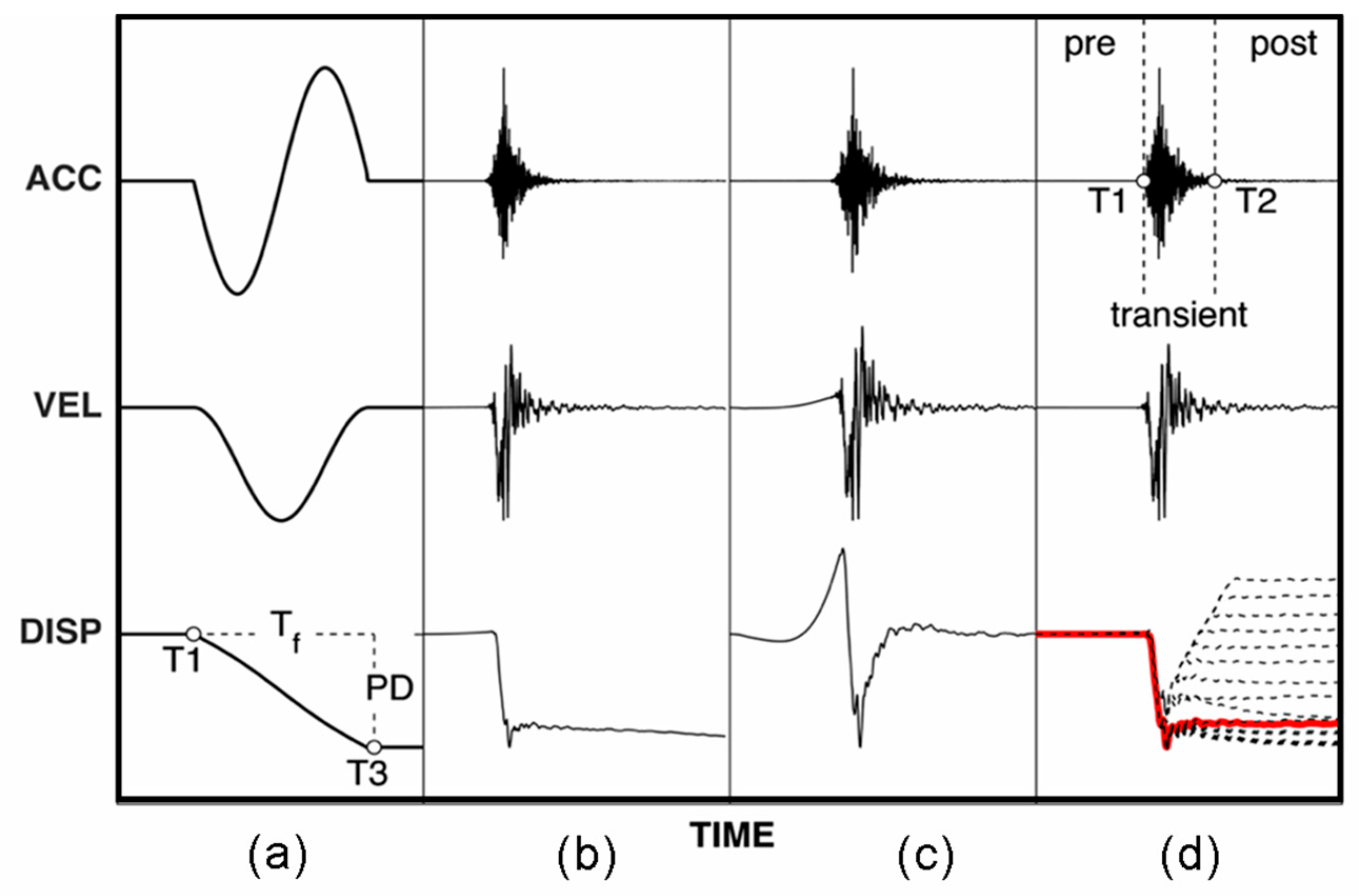
Commonly, strong ground-motion records are affected by high- and low-frequency noise as well as by non-standard errors (e.g., spurious spikes, multiple baselines, etc.), so that data processing is always necessary to be able to employ such recordings in any engineering analysis. In the last decades, many studies on the processing of recorded accelerograms have been published. However, each scheme features its own advantages and limitations, as well as a certain degree of subjectivity, making the identification of standard procedures difficult [1]. Currently, most of the processing tools for accelerometric data remove the low-frequency content of the signal (e.g., [2,3,4,5,6]), leading to a loss of information related to near-source records. Indeed, near-source ground motion may be affected by two different effects, which can lead to large and long period pulses: rupture directivity and tectonic fling. The former produces short-duration and large-amplitude two-side pulses in the velocity trace along the fault-normal direction; the latter is the expression of the permanent tectonic offset of a rupturing fault and it is usually characterized by a one-side pulse in the velocity trace and by a non-zero final displacement along the slip direction (e.g., [7,8,9]). While directivity effects are usually fully recovered by conventional processing schemes, the accurate recovery of the flying is made difficult by the presence of noise and baseline offsets that, although small in acceleration, lead to artificial long period drifts in the displacement trace [9,10,11,12,13] (Figure 1).

Preserving the low-frequency information of a waveform and thus quantifying the near-source fling step is of great interest for both engineering seismology and structural engineering applications. Indeed, velocity pulses and residual static deformations can potentially be more damaging for base-isolated buildings, large-scale structures, such as long-span bridges and lifeline infrastructures, and geotechnical systems, such as underground and retaining structures [8,14,15]. The permanent displacement (PD) from acceleration waveforms, in addition to Global Positioning System (GPS) and Interferometric Synthetic Aperture Radar (InSAR) data, can be employed to better constrain fault-slip distribution and thus to refine the resolution of finite-fault slip inversion [13]. Dhanya and Raghukanth [16] proposed a new probabilistic fling hazard map for the India region that can potentially be used in the displacement-based design of structures.

Studies on how to recover permanent displacements from strong motion data and methods for baseline correction have been published since the 1970s, right after the development of the modern digital recordings [17]. Among the principal approaches based on piecewise correction of the signal baseline, noteworthy are Graizer [18], Iwan et al. [19], Boore [10], Graves [11], Wu and Wu [17], Chen and Loh [20], Chao et al. [21], Rupakhety et al. [22], Wang et al. [12] and D’Amico et al. [9]. A review of some of such studies with emphasis on their limitations can be found in [22]. Recently, Inbal and Ziv [13] proposed a novel methodology based on the bilinear correction approach of [19] and subsequently improved by [12,17]. However, the new scheme works in the frequency domain for the selection of time correction points, as opposed to the time domain.

Despite the still ongoing research, properly estimating the uncertainties in the static deformation data is still a controversial issue; different baseline correction approaches may return variable PD since the seismic displacement is a very sensitive ground-motion characteristic. In such a context, GPS and InSAR data could be employed as a benchmark to obtain reliable displacement traces from accelerograms [9,12,13]. However, the availability of GPS receivers close to accelerometric stations is, generally, quite scarce. Besides, ground motion simulations represent an effective tool to quantify the static displacement in the absence of observations, as they embody physical and sufficiently accurate models of the seismic source, path and local-site effects.

Nowadays, there are very few PD predictive models mainly due to: (1) the shortage of near-source records that contain fling effects, and (2) the limitations in retrieving the static displacement from accelerometric data. Kamai et al. [8] and Burks and Baker [23] proposed simplified fling steps models, which were mostly calibrated on ground motion simulations of strike-slip and reverse scenarios. Recently, Dhanya and Raghukanth [16] developed a new fling prediction equation that is also based on simulated events consistent with the tectonics of India.

In this work, we present the recent update of an automatic processing scheme, extended BASeline COrrection (eBASCO), for piecewise baseline correction of near-source records [9]. Its main advantage lies with the possibility to automatically process a considerable number of signals in a very short time. We extensively test eBASCO against about 600 high-quality near-source records with a magnitude ranging between 5.5 and 8.1 and within a R_JB (Joyner and Boore) distance of 140 km coming from the most updated version of the NESS dataset [24]. NESS represents the most comprehensive dataset of ground motion parameters and associated metadata related to more than 1000 near-source three-component waveforms from moderate-to-large magnitude events recorded worldwide and collected from public archives. While strike-slip events dominate the data processed by means of eBASCO, the uniqueness of it lies with the availability of 120 records from 15 normal-faulting earthquakes. Such events are indeed poorly represented in worldwide databases. We test our approach against geodetic measurements as well as existing predictive models to assess its robustness. In addition, we propose a comparison with the standard processing scheme adopted in NESS based on a passband filtering and tapering at the end of the signal [5] to test the capability of eBASCO to preserve the long-period ground-motion in near-source regions.

The main goal of this work is two-fold: (1) developing a sound methodology to process near-source strong motion data, preserving the low-frequency content of the signals, and (2) compiling a database of fling-step-containing records that may be employed to calibrate attenuation models specifically tailored for the low-frequency content of the ground-motion. Finally, we note that the eBASCO code can be easily integrated in the web interface of the Engineering Strong Motion (ESM) database (https://esm-db.eu/ (accessed on 29 December 2020)) to make alternative processing schemes for strong motion waveforms available to the User.

2. What eBASCO Does and What Problems It Solves

eBASCO (extended BASeline COrrection) removes the baseline of strong-motion records due to many different factors such as instrumental effects, ground rotation and tilting, by means of a tri-linear detrending of the velocity time series. Differently from standard processing schemes, eBASCO does not apply any filtering to remove the low-frequency content of the signal and taper windowing at the end of the signal. This approach preserves the long-period near-source ground-motion featured by a one-side pulse in the velocity trace (fling-step) and an offset at the end of the displacement trace (Figure 1).

The eBASCO processing scheme (Figure 2) can be summarized in four main steps:

• Cut of the uncorrected accelerometric waveform
• Sampling of the Time Correction Points
• Tri-Linear Detrending of the velocity
• Selection of the best solution

The eBASCO procedure is very sensitive to the preliminary cutting of the accelerometric waveforms to isolate the uncorrected earthquake records; a bad cutting may cause unwanted distortion of the signal. As a default, eBASCO applies an automatic cutting of the three components of the uncorrected accelerometric waveform based on the cumulative ground motion energy. Otherwise, a manual cutting can be applied after visual inspection of the waveform.

The baseline distortion of the acceleration trace is subdivided into three time-windows: (1) pre-event window between the time of the first sample T₀ and the time T₁ when the ground starts to move toward the final displacement; (2) transient-window containing the strong phase of the motion between T₁ and the time T₂ at which the ground has already reached the final displacement; (3) post-event window from T₂ and the end of the signal (T_end). The selection of the two correction points T₁ and T₂ follows a recursive procedure described in [17,21] and modified in [9]. T₁ is sampled before the time at which the cumulative acceleration energy reaches 5% of the total energy (logarithmically spaced between 0.001% and 5%), whereas T₂ is sampled after a further time point T₃, which represents the time at which the ground has just reached the final deformation. T₃ is logarithmically sampled between the times at which the cumulative energy distribution reaches 50% and 95% of the total energy.

Once the time correction points are identified, eBASCO applies a linear detrend of the velocity trace in each time window. The amplitude of the first sample is primarily removed from the whole acceleration so that the velocity equals zero in T₀. The signal distortion in the pre-event window is removed by subtracting from the velocity trace a regression line (1) crossing the first sample V(T₀) = 0:

V(t) = A_it,

(1)

where A_i is the slope of the line fitting the velocity between T₀ and T₁. A further least-squares fitting (2) is used to remove the velocity drift in the post-event window:

V_f(t) = V_0,f + A_ft

(2)

where V_0,f is the intercept and A_f is the slope of the line fitting the velocity between T₂ and T_end.

The baseline correction applied to the transient-window is given by a linear trend between V_i(T₁) and V_f(T₂); such points are the pre-event baseline correction (1) evaluated at t = T₁ and the post-event detrending line (2) evaluated at t = T₂, respectively.

The velocity time series determined by all the T₁ and T₂ correction point combinations are differentiated to obtain the acceleration. Because inappropriate combinations of correction points might generate spurious spikes in the acceleration trace, a threshold on the amplitudes in T₁ and T₂ should be set. As the default, eBASCO considers all the acceleration waveforms for which the relative difference between the amplitude in T₁ and T₂ before and after the eBASCO processing is lower than 25% as acceptable. Only the acceptable solutions are double-integrated to obtain the ground displacement. We compute a flatness indicator [17] on the displacement trace between T₃ and T_end to guarantee that the eBASCO displacement waveform features a ramp function:

$$\mathrm{f}=\frac{\mathrm{r}}{\left|\mathrm{b}\right|\times \mathsf{\sigma }}$$

(3)

where r is the linear correlation coefficient of the displacement amplitudes, b is the slope of the linear fit, and $\mathsf{\sigma }$ is the variance of the residual displacement with respect to the mean value. The more the absolute value of r and b tends to 1 and 0, respectively, and $\mathsf{\sigma }$ tends to lower values, the flatter the displacement waveform is. We consider the acceleration corresponding to the displacement trace with the maximum f-value over all the T₁ and T₂ correction points combinations as the best solution.

Finally, eBASCO applies a second-order low-pass filter (acausal Butterworth) and a recursive integration to the best solution to obtain the final velocity and displacement. Each integration step implies also the application of a cosine taper at the beginning of the trace.

The processing scheme here described has been implemented in a python2.7 code named eBASCO.py (version 1.0) and it is available as electronic supplement (Annex S1: eBASCO.zip). An example of the command line and the parameters that need to be set within eBASCO is provided in

Table A1. Example of a command line to run eBASCO.py.

Usage Example: Python eBASCO.py [Options]
Usage Example: Python eBASCO.py --ifile = [INPUT_DIR]/IT.CLO.00.HG.EMSC-20161026_0000095.h5 --ofldr = [OUTPUT_DIR] --t1 = 5 --t2 = 20 --t3 = 20 --eps = 0.25 --mfst = 1.5 --mfnd = 2.0 --ca = 0 --cz = 0 --ta = 5 --he = 35 --hn = 35 --hz = 35 --fo = 2
Options	Description	Default	Format
--ifile	ASDF file containing the waveforms to be processed		str
--ofldr	Destination folder for the eBASCO output		str
--t1	number of T1 correction points samples	5	int
--t2	number of T2 correction points samples	20	int
--t3	number of T3 correction points samples	20	int
--eps	maximum threshold of the relative difference between acceleration in T1 and T2 correction points before and after the eBASCO processing	0.25	float
--mfst	multiplier factor to cut the beginning of the waveform on the base of the energy criterion. Firstly the significative duration T90 of the seismic motion is calculated on the base of the normalized Arias Intensity I(t) between in the time interval t2 − t1, where I(t1) = 0.05 and I(t2) = 0.95; after that the cut at the beginning is set at the time t1 − mfst × T90	1.5	float
--mfnd	multiplier factor to cut the beginning of the waveform on the base of the energy criterion. Firstly the significative duration T90 of the seismic motion is calculated on the base of the normalized Arias Intensity I(t) in the time interval t2 − t1, where I(t1) = 0.05 and I(t2) = 0.95; after that the cut at the beginning is set at the time t1 − mfnd × T90	2.0	float
--ca	seconds to cut from the beginning of the waveforms; ca is used only if different from the default value, otherwise eBASCO use the energy criterion to cut the strong-phase of motion between the 5% and the 95% of the energy release	0	float
cz	seconds to cut from the end of the waveforms; cz is used only if different from the default value, otherwise eBASCO use the energy criterion to cut the strong-phase of motion between the 5% and the 95% of the energy release	0	float
ta	percentage of the signal length to set the time window at the beginning of the waveform where a cosine taper will be applied	5	float
he	cutoff frequency of the low-pass Butterworth filter (first component)	35	float
hn	cutoff frequency of the low-pass Butterworth filter (second component)	35	float
hz	cutoff frequency of the low-pass Butterworth filter (third component)	35	float
fo	Butterworth filter order	2	float

in Appendix A. eBASCO.py requires as input file an Adaptable Seismic Data Format (ASDF, https://seismic-data.org/ (accessed on 29 December 2020); [25]) with the same HDF5 (Hierarchical Data Format version 5; The HDF Group 1997–2015) structure adopted by the Engineering Strong Motion database (ESM, https://esm-db.eu (accessed on 29 December 2020)). The ESM ASDF volumes are organized in three sections related to the events, waveforms, and auxiliary data. Information about an arbitrary number of seismic events is in a QuakeML structure, while accelerometric waveforms are stored for each single station together with an FDSN (International Federation of Digital Seismograph Network) StationXML (https://www.fdsn.org/xml/station/ (accessed on 29 December 2020)). Each waveform is a piece of a continuous trace regularly sampled and recorded by a seismic instrument within the time interval [start_time; end_time]. Each station may contain an arbitrary number of traces related to multiple channels. Each trace is identified by a waveform tag with the following structure:

‘location_code’_’channel_code’_’event_id’_’file_type’_’processing_type’

where the sequence of placeholders indicates the specific record of a station, the seismic event, the ground motion parameters, and the processing workflow, respectively (

Table A2. Example of ASDF waveform tag.

Placeholders	Description	Example
net_code	code associated to the recording network according to the International Federation of Seismograph Network (http://www.fdsn.org (accessed on 29 December 2020))	IT
station_code	3 to 5 characters to identify the recording station	CLO
location_code	0 to 2 characters to identify a specific recording instrument at a station; Note that double-zeros are always replaced by empty strings	00
channel_code	3 digits to indicate the band code, the instrument code (N, L, G for accelerometer), and the orientation code (e.g., Z, N, E for the specific orientation Vertical, North-Shout, East-West or Z, 2, 3 for generic orthogonal orientation)	hnn
event_id	alphanumeric code to identify the seismic event	emsc_20161026_0000095
file_type	2 to 3 characters to indicate the ground motion parameter of time series (ACC: acceleration; VEL: velocity; DIS: displacement) or 5% damped response spectra (SA: acceleration; SD: displacement)	acc
processing_type	2 characters to indicate the type of data processing (CV: acceleration ConVerted in physical units; MP or AP: acceleration Manually or Automatically processed using the workflow proposed in Ref. [5]; MB or AB: acceleration Manually or Automatically processed by means eBASCO	cv

). All the meta information related to the waveforms are hierarchically stored in the Auxiliary Data section (Headers) together with 5% damped acceleration and displacement response spectra (Spectra). Both Headers and Spectra are identified within the two relative data groups by the corresponding waveform tags.

3. Fling-Step Containing Waveforms and Comparison with GPS Data

We applied eBASCO to worldwide, near-source, high-quality, strong-motion waveforms archived in NESS [24] and to a selection of other relevant records such as the Mw 7.58 1999 Chi-Chi earthquake (https://gdms.cwb.gov.tw/ (accessed on 29 December 2020)). We processed about 600 three-component waveforms of 65 moderate-to-large earthquakes with (1) moment magnitude between 5.5 and 8.1, (2) hypocentral depth shallower than 30 km, and (3) Joyner–Boore distance up to nearly 140 km. The majority of data are characterized by a fault distance smaller than 10 km and by a moment magnitude in the range 5.5–7.0. Although the prevailing style of faulting is strike-slip, normal and reverse mechanisms are also well represented. A summary of the selected events is reported in

Table 1. Earthquakes selected for the fling-step recovery.

Event ID	Event Name	Territories	Event Date	Lat [°]	Lon [°]	FM	M	# rec
EMSC-20070716_0000038	Niigata-Chuetsu Oki	Japan	16/07/2007 01:13	37.56	138.61	TF	6.6	1
EMSC-20080613_0000091	Iwate–Miyagi Nairiku	Japan	13/06/2008 23:43	39.03	140.88	TF	6.9	12
EMSC-20100903_0000044	Darfield	New Zealand	03/09/2010 16:35	−43.53	172.17	SS	7.1	13
EMSC-20110221_0000047	Christchurch	New Zealand	21/02/2011 23:51	−43.58	172.68	TF	6.2	6
EMSC-20110222_0000004	Christchurch	New Zealand	22/02/2011 01:50	−43.59	172.74	SS	5.6	1
EMSC-20110411_0000023	Fukushima	Japan	11/04/2011 08:16	36.95	140.67	NF	6.6	7
EMSC-20110613_0000006	Christchurch	New Zealand	13/06/2011 02:20	−43.50	172.78	SS	6	8
EMSC-20140126_0000046	Kefallonia	Greece	26/01/2014 13:55	38.15	20.39	SS	6.19	1
EMSC-20140401_0000093	Iquique	Chile	01/04/2014 23:46	−19.58	−70.79	TF	8.1	5
EMSC-20140524_0000026	Aegean Sea	Greece	24/05/2014 09:25	40.29	25.39	SS	6.5	2
EMSC-20140824_0000036	South Napa	United States	24/08/2014 10:20	38.22	−122.31	SS	6.07	9
EMSC-20150425_0000021	Gorkha	Nepal	25/04/2015 06:11	28.28	84.79	TF	7.8	1
EMSC-20160824_0000006	Accumoli	Italy	24/08/2016 01:36	42.70	13.23	NF	6	7
EMSC-20161026_0000095	Visso	Italy	26/10/2016 19:18	42.91	13.13	NF	5.9	14
EMSC-20161030_0000029	Norcia	Italy	30/10/2016 06:40	42.83	13.11	NF	6.5	47
EMSC-20161113_0000048	Kaikoura	New Zealand	13/11/2016 11:02	−42.74	173.05	SS	8	32
EMSC-20170118_0000034	Capitignano	Italy	18/01/2017 10:14	42.53	13.28	NF	5.5	7
EMSC-20190706_0000043	Ridgecrest	United States	06/07/2019 03:19	35.79	−117.58	SS	7.1	24
EMSC-20201030_0000082	Aegean Sea	Turkey	30/10/2020 11:51	37.91	26.84	NF	7	1
GR-1986-0006	Kalamata	Greece	13/09/1986 17:24	37.08	22.15	NF	5.9	1
GR-1995-0047	Aigio	Greece	15/06/1995 00:15	38.40	22.27	NF	6.5	1
INT-UT19990920_174715	Chi-Chi	Taiwan	20/09/1999 17:47	23.83	120.81	TF	7.5	151
INT-UT19991022_021856	Chi-Chi	Taiwan	22/10/1999 02:18	23.52	120.43	TF	6.1	6
IR-2003-0041	Bam	Iran	26/12/2003 01:56	28.98	58.36	SS	6.5	1
IR-2004-0043	Baladeh	Iran	28/05/2004 12:38	36.32	51.59	TF	6.4	1
IR-2005-0044	Zarand	Iran	22/02/2005 02:25	30.77	56.81	TF	6.5	3
IT-1976-0027	Friuli 2nd shock	Italy	15/09/1976 03:15	46.29	13.20	TF	5.9	1
IT-1976-0030	Friuli 3rd shock	Italy	15/09/1976 09:21	46.30	13.17	TF	6	2
IT-1984-0005	Abruzzo-Lazio	Italy	11/05/1984 10:41	41.78	13.89	NF	5.5	1
IT-1997-0004	Umbria-Marche 1st shock	Italy	26/09/1997 00:33	43.02	12.89	NF	5.7	1
IT-1997-0006	Umbria-Marche 2nd shock	Italy	26/09/1997 09:40	43.03	12.86	NF	6	2
IT-1997-0137	Umbria-Marche 3th shock	Italy	14/10/1997 15:23	42.93	12.93	NF	5.6	1
IT-2009-0009	L’Aquila	Italy	06/04/2009 01:32	42.34	13.38	NF	6.1	5
IT-2009-0102	Cental Italy	Italy	07/04/2009 17:47	42.30	13.49	NF	5.5	7
IT-2012-0008	Emilia 1st shock	Italy	20/05/2012 02:03	44.90	11.26	TF	6.1	1
IT-2012-0010	Cavezzo	Italy	29/05/2012 10:55	44.87	10.98	TF	5.5	6
IT-2012-0011	Emilia 2nd shock	Italy	29/05/2012 07:00	44.84	11.07	TF	6	18
JP-2000-0007	Tottori	Japan	06/10/2000 04:30	35.28	133.35	SS	6.6	8
JP-2004-0002	Niigata	Japan	23/10/2004 08:55	37.29	138.87	TF	6.6	11
JP-2004-0003	Niigata	Japan	27/10/2004 01:40	37.29	139.04	TF	5.8	1
JP-2005-0002	Fukuoka	Japan	20/03/2005 01:53	33.74	130.18	SS	6.6	1
TK-1999-0077	Izmit	Turkey	17/08/1999 00:01	40.76	29.96	SS	7.6	10
TK-1999-0294	Kocaeli	Turkey	13/09/1999 11:55	40.75	30.08	NF	5.8	1
TK-1999-0415	Düzce	Turkey	12/11/1999 16:57	40.81	31.19	SS	7.3	8
TK-2003-0038	Bingöl	Turkey	01/05/2003 00:27	39.00	40.46	SS	6.3	1
USGS-iscgem787038	San Fernando	United States	09/02/1971 14:00	34.40	−118.43	TF	6.7	3
USGS-iscgem893168	Kern County	United States	21/07/1952 11:52	34.99	−119.02	TF	7.3	1
USGS-nc51147892	Parkfield	United States	28/09/2004 17:15	35.82	−120.37	SS	5.9	40
USGS-us20005i1a	Kumamoto	Japan	14/04/2016 15:03	32.70	130.72	SS	6	6
USGS-us20005iis	Kumamoto	Japan	15/04/2016 16:25	32.75	130.76	SS	7	31
USGS-usp0000w1w	Santa Barbara	United States	13/08/1978 22:54	34.40	−119.68	TF	5.8	2
USGS-usp000128g	Coyote Lake	United States	06/08/1979 17:05	37.07	−121.49	SS	5.8	3
USGS-usp00013ee	Imperial Valley	Mexico	15/10/1979 23:16	32.64	−115.31	NF	6.5	18
USGS-usp000181t	Alberto Oviedo Mota	Mexico	09/06/1980 03:28	32.19	−115.08	SS	6.3	1
USGS-usp0001dcq	Westmorland	United States	26/04/1981 12:09	33.10	−115.62	SS	5.9	2
USGS-usp0002vtg	North Palm Springs	United States	08/07/1986 09:20	34.00	−116.61	TF	6.7	6
USGS-usp0003afe	Superstion Hills	United States	24/11/1987 13:15	33.02	−115.85	SS	6.6	1
USGS-usp00040t8	Loma-Prieta	United States	18/10/1989 00:04	37.04	−121.88	TF	6.9	19
USGS-usp000566s	Joshua Tree	United States	23/04/1992 04:50	33.96	−116.32	SS	6.1	1
USGS-usp00056e1	Cape Mendocino	United States	25/04/1992 18:06	40.33	−124.23	TF	7	3
USGS-usp00056fp	Cape Mendocino	United States	26/04/1992 07:41	40.43	−124.57	SS	6.5	1
USGS-usp00056g0	Cape Mendocino	United States	26/04/1992 11:18	40.38	−124.56	SS	6.7	1
USGS-usp00059sn	Landers	United States	28/06/1992 11:57	34.20	−116.44	SS	7.3	1
USGS-usp00066k9	Northridge	United States	17/01/1994 12:30	34.21	−118.55	TF	6.7	12
USGS-usp000bg0m	Denali	United States	03/11/2002 22:12	63.52	−147.44	TF	7.8	2

, whereas the distributions of the selected data with respect to distance, magnitude, fault mechanism and magnitude-distance are summarized in Figure 3.

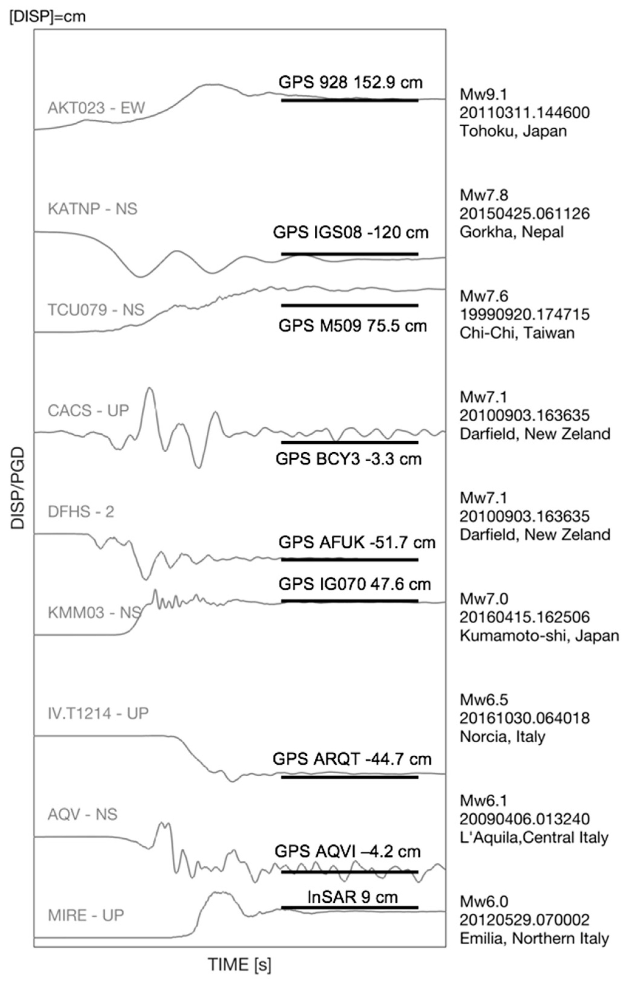
We compare the static offset of the displacement waveforms with nearby geodetic measurements of different moderate-to-large worldwide earthquakes to evaluate the effectiveness of eBASCO (Figure 4). We observe a general agreement between accelerometric records and geodetic measurements, both in terms of amplitude and sense of movement. In addition, we perform a cross-correlation analysis between strong-motion and High-Rate GPS (HRGPS) time series available from the RING (Rete Integrata Nazionale GNSS; http://0-doi-org.brum.beds.ac.uk/10.5281/zenodo.268045 (accessed on 29 December 2020)) database for the 2016 Norcia earthquake (30 October, 06:40 UTC, Mw 6.5). Such comparison allows assessing the capability of the eBASCO processing scheme to reproduce both the dynamic and static parts of the ground motion. Indeed, we compute the normalized cross-correlation function (NCC) for two different portions of the signals following the procedure described in [26]: (1) between T1 and T2 and (2) between T3 and the end of the signal. The former gives a measure of the similarity of the time histories in the dynamic part of the ground motion, whereas the latter tests the ability of eBASCO to recover the fling step. Figure 5 presents the comparison between the seismic station IV.T1214 and the GPS station RIFP, located only ~2.5 km away from each other. The matching between the EW and UP components is noteworthy, with NCC values very close to one, both in the transient and post-event windows. For the sake of completeness, we report in Figure 5 (green line) the corresponding displacement waveform processed following the standard procedure described in [5] that removes the low-frequency content of the signal. Other comparisons between strong-motion and HRGPS time series are reported in Appendix B.

4. Results

4.1. Comparison with Standard Processing Schemes

In Figure 6, we compare the peak ground acceleration (PGA), velocity (PGV) and displacement (PGD) obtained from eBASCO with the NESS corresponding values, which are manually processed by applying a second-order acausal time-domain Butterworth filter to the zero-padded acceleration time series and a cosine taper at both the beginning and the end of the signal [5,6]. The aim of such comparison is twofold: (1) to highlight the differences among the two adopted processing schemes, and (2) to test the capability of eBASCO to preserve the long-period ground-motion of near-source records. We show the results in terms of fault-normal (FN), fault-parallel (FP) and vertical (UP) ground motion components, since the fling-step is typically observed along the FP direction for strike-slip faults and along the FN and UP directions for dip-slip faults [7]. As expected, PGAs are insensitive to the different low-frequency treatment of the signal, being related to higher frequencies. Conversely, PGDs_eBASCO are larger than PGDs_NESS because eBASCO preserves the information related to both the static and dynamic displacement. We note a dispersion along the first bisector (45° line) for PGV values also. PGVs are indeed related to intermediate frequencies and as a result, they may be slightly affected by the base-line correction.

Furthermore, we performed a comparison between displacement response spectra (Sd) obtained from eBASCO and NESS (Figure 7). The differences between the approaches amplify as the oscillating period increases, indicating that our processing scheme provides larger spectral ordinates compared to the standard approach. This is a rather expected result as it is well known that the maximum response of an oscillator should approach the PGD value at long periods. The displacement spectra start diverging at T = 2 s and they differ by about 7% (14%, 11%) at T = 4 s up to 88% (74%, 123%) at T = 10 s on average for the FN (FP, Z) component. In terms of fault mechanism, normal and reverse faults show larger discrepancies along the FN and UP directions, whereas strike-slip faults feature larger differences along the FP directions, consistent with the physics of the problem. We find also a dependency on the magnitude: higher magnitude events are characterized by larger differences in terms of Sd values. The figures are not reported here for the sake of brevity.

4.2. Comparison with Attenuation Models

We compare the eBASCO outcomes with two different fling-step models proposed by Kamai et al. [8] and Burks and Baker [23]. Such attenuation relationships are mostly calibrated on simulations of reverse and strike-slip scenarios with magnitude between 6.0–8.2 [8] and 7.0–8.3 [23]. Permanent displacements recovered by eBASCO and those predicted by the Burks and Baker model are, to some extent, in agreement only for R_JB distances larger than 10 km and for magnitudes greater than 6.0 (Figure 8a,c). The observed PDs decay faster with distance compared to the predictive model, whereas the PD values at stations very close to the fault trace (|Rx| < 20 km) are generally underestimated both in hanging- and foot-wall (Figure 8b,d). It must be observed that the lower magnitude bins (Mw 5.5–7.0) are outside the validity range of the predictive model, so that more care should be taken when comparing observed and predicted PDs. In particular, the lowest magnitudes are affected by a considerable bias close to the fault trace that depends on the large variability of the PDs values under 1 cm. In addition, our dataset presents a large number of recordings from normal fault earthquakes that may lead to a greater variability in the residuals, as the model is calibrated on reverse and strike-slip events. Nonetheless, the comparison between the PD values larger than 1 cm and the prediction is rather satisfactory, supporting the reliability of the processing scheme.

The predictive model developed in [8] introduces the fault dip as an explanatory variable in addition to the magnitude and distance. Consequently, the comparison between observed and predicted PDs can also be interpreted in terms of asymmetry degree between Hanging-Wall (HW) and Foot-Wall (FW) and as a function of the dipping fault geometry. Figure 9 presents both the horizontal and vertical eBASCO PDs values as a function of both the rupture distance (R_RUP) and dip angle. We also plot the corresponding predictive models of strike-slip and reverse faulting with different values of dip, fixing a Mw = 7.0. Generally, the predictive model describes the attenuation of the horizontal PD amplitudes reasonably well in the case of strike-slip mechanisms. Even though the comparison of vertical and horizontal PD values with the corresponding model for the reverse fault mechanism is rather satisfactory, we notice that (1) the eBASCO PD amplitudes tend to decay faster with respect to the predicted values, and (2) the predictions tend to either underestimate or overestimate the recorded displacement (i.e., in the HW side of reverse fault with dipping angle of about 60° both for horizontal and vertical components). Nonetheless, the fling-step amplitudes are larger for HW stations with respect to the FW ones, as demonstrated by [8]. Eventually, the analysis of the residuals computed as the log difference between observed and predicted PD values shows a large variability. We recall that the predictive model of [8] is calibrated on finite-fault simulations and for this reason, it may not sample all the variability observed in the real world. The distributions of the residuals as a function of the relative position of the station with respect to the fault plane (FW or HW), magnitude and dip angle are presented in Figure 10.

5. Discussion

In this technical note, we present the recent update of eBASCO, an automatic processing scheme for piecewise baseline correction of near-source records [9]. The main advantages of the proposed processing scheme compared to other approaches are the following: (1) its objectiveness in the selection of the correction points, and (2) its capability to automatically process a considerable number of waveforms in a very short time. The latter is of fundamental importance to populate strong-motion databases (i.e., https://esm-db.eu/ (accessed on 29 December 2020)) with long-period, high-quality data, which are useful for both engineering and seismological purposes.

We apply eBASCO to a worldwide near-source strong-motion database (NESS, [24]) and to a selection of other relevant records to test its ability to preserve the low-frequency content of the waveforms and thus estimate the fling-step. The comparison of our results with GPS and InSAR data provides a good agreement, suggesting that eBASCO allows preserving the offset in the displacement trace. Furthermore, our results are also comparable with those of other studies, such as [22], who analyzed both strong-motion and GPS data from the 1999 Chi Chi earthquake.

The analyses of the results demonstrate that, in general, PGDs_eBASCO are larger than PGDs_NESS. Indeed, standard processing schemes remove the low-frequency content of the signal and force the velocity and displacement to return to zero, leading to a loss of information related to both the static (PD) and dynamic (PGD) displacement. Conversely, we do not find any differences in terms of PGAs, as such values are related to higher frequencies.

Furthermore, our processing scheme provides larger spectral ordinates compared to the standard approach. We note that the spectra start diverging from an oscillator period longer than ~4 s, depending both on the magnitude and faulting mechanism. Our outcomes differ from several other studies, such as [10] and [22], who claim that the long-period spectral ordinates depend slightly on the adopted correction procedures, in contrast to the relevant effect of the latter on the displacement waveforms. In [10], it was demonstrated that spectral ordinates with a period of less than ~20 s are usually insensitive to different processing schemes, so that the uncertainties in response spectra due to baseline shifts do not affect periods of interest for engineering purposes. Likewise, [22] found that inelastic spectral displacements are also not sensitive to different schemes of baseline correction. Such comparison supports the need to improve the accuracy of near-source, strong-motion waveform processing to preserve the long-period information and hence provide reliable estimates of both fling-step amplitudes and displacement spectral ordinates.

Nowadays, there are very few predictive models for the final offset of the ground displacement and the one-side pulse in the velocity trace that occur during an earthquake, mainly due to the difficulties in detecting the fling-step in near-source waveforms. In addition, these models are largely derived from ground-motion simulations based on strike-slip and reverse-faulting scenarios. Although the comparison between observations and predictions is rather satisfactory, calibrating attenuation models specifically tailored for the low-frequency content of the ground-motion and uniquely based on large databases represents a challenging task. For such reason, our main goal is to provide a sound methodology to process near-source strong motion data, preserving the low-frequency content of the signals and, consequently, integrate existing datasets (NESS, [24]) with such long-period intensity measures. Such a flat-file could be useful to (1) update existing empirical equations for the prediction of the final displacement and pulse duration [8,23]; (2) develop new PD attenuation models, which also take normal fault scenarios into account; and (3) provide empirical coefficients to adjust displacement response spectral ordinates from existing prediction models (e.g., [29,30]), similarly to [31], who provide empirical correction factors for pulse-like ground motion records. In particular, further developments of the long-period data processing scheme will allow for the detection of near-source waveforms affected by one-side velocity pulses before applying the baseline-correction.

This technical note is part of the preparatory phase that leads to the compilation of a qualified dataset of permanent ground displacement and displacement spectra ordinates, which are the result of a robust and homogeneous procedure specifically tailored to preserve the low-frequency content of fling-contains waveforms. The eBASCO flat-file [32] is released in the framework of the DPC-ReLUIS Agreement 2019–2021 and is available at the following link http://ness.mi.ingv.it/ (accessed on 29 December 2020). This is of great interest for a variety of engineering applications, such as the performance-based seismic design to assess the likely performance of an existing building structure during an earthquake.

References

- Massa, M.; Pacor, F.; Luzi, L.; Bindi, D.; Milana, G.; Sabetta, F.; Gorini, A.; Marcucci, S. The ITalian ACcelerometric Archive (ITACA): Processing of strong-motion data. Bull. Earthq. Eng. 2009, 8, 1175–1187. [Google Scholar] [CrossRef]
- Boore, D.M.; Bommer, J.J. Processing of strong-motion accelerograms: Needs, options and consequences. Soil Dyn. Earthq. Eng. 2005, 25, 93–115. [Google Scholar] [CrossRef]
- Akkar, S.; Bommer, J.J. Influence of long-period filter cut-off on elastic spectral displacements. Earthq. Eng. Struct. Dyn. 2006, 35, 1145–1165. [Google Scholar] [CrossRef]
- Douglas, J.; Boore, D.M. High-frequency filtering of strong-motion records. Bull. Earthq. Eng. 2010, 9, 395–409. [Google Scholar] [CrossRef] [Green Version]
- Paolucci, R.; Pacor, F.; Puglia, R.; Ameri, G.; Cauzzi, C.; Massa, M. Record processing in ITACA, the new Italian strong-motion database. In Earthquake Data in Engineering Seismology: Predictive Models, Data Management and Networks; Akkar, S., Gülkan, P., van Eck, T., Eds.; Springer: Dordrecht, The Netherlands, 2011; pp. 99–113. ISBN 978-94-007-0151-9. (printed version); 978-94-007-0152-6 (e-book version). [Google Scholar]
- Puglia, R.; Russo, E.; Luzi, L.; D’Amico, M.; Felicetta, C.; Pacor, F.; Lanzanó, G. Strong-motion processing service: A tool to access and analyse earthquakes strong-motion waveforms. Bull. Earthq. Eng. 2018, 16, 2641–2651. [Google Scholar] [CrossRef]
- Somerville, P.G. Engineering characterization of near fault ground motions. In Proceedings of the 2005 NZSEE Conference, Taupo, New Zealand, 11–13 March 2005; pp. 1–8. [Google Scholar]
- Kamai, R.; Abrahamson, N.; Graves, R. Adding Fling Effects to Processed Ground-Motion Time Histories. Bull. Seism. Soc. Am. 2014, 104, 1914–1929. [Google Scholar] [CrossRef]
- D’Amico, M.; Felicetta, C.; Schiappapietra, E.; Pacor, F.; Gallovič, F.; Paolucci, R.; Puglia, R.; Lanzano, G.; Sgobba, S.; Luzi, L. Fling Effects from Near-Source Strong-Motion Records: Insights from the 2016 Mw 6.5 Norcia, Central Italy, Earthquake. Seism. Res. Lett. 2018, 90, 659–671. [Google Scholar] [CrossRef]
- Boore, D.M. Effect of Baseline Corrections on Displacements and Response Spectra for Several Recordings of the 1999 Chi-Chi, Taiwan, Earthquake. Bull. Seism. Soc. Am. 2004, 91, 1199–1211. [Google Scholar] [CrossRef] [Green Version]
- Graves, R.W. Processing Issues for Near Source Strong Motion Recordings. In Proceedings of the COSMOS Workshop on Strong-Motion Record Processing, Richmond, CA, USA, 26–27 May 2004. [Google Scholar]
- Wang, R.; Schurr, B.; Milkereit, C.; Shao, Z.; Jin, M. An Improved Automatic Scheme for Empirical Baseline Correction of Digital Strong-Motion Records. Bull. Seism. Soc. Am. 2011, 101, 2029–2044. [Google Scholar] [CrossRef]
- Inbal, A.; Ziv, A. Automatic Extraction of Permanent Ground Offset from Near-Field Accelerograms: Algorithm, Validation, and Application to the 2004 Parkfield Earthquake. Bull. Seism. Soc. Am. 2020, 110, 2638–2646. [Google Scholar] [CrossRef]
- Akkar, S.; Boore, D.M. On Baseline Corrections and Uncertainty in Response Spectrafor Baseline Variations Commonly Encounteredin Digital Accelerograph Records. Bull. Seism. Soc. Am. 2009, 99, 1671–1690. [Google Scholar] [CrossRef]
- Wu, S.-L.; Nozu, A.; Nagasaka, Y. Accuracy of Near-Fault Fling-Step Displacements Estimated Using the Discrete Wavenumber Method. Bull. Seism. Soc. Am. 2020, 1–12. [Google Scholar] [CrossRef]
- Dhanya, J.; Raghukanth, S.T.G. Probabilistic Fling Hazard Map of India and Adjoined Regions. J. Earthq. Eng. 2020, 1–25. [Google Scholar] [CrossRef]
- Wu, Y.; Wu, C.-F. Approximate recovery of coseismic deformation from Taiwan strong-motion records. J. Seism. 2007, 11, 159–170. [Google Scholar] [CrossRef]
- Graizer, G.M. Determination of the true ground displacement by using strong motion records. Izv. Phys. Solid Earth 1979, 15, 875–886. [Google Scholar]
- Iwan, W.D.; Moser, M.A.; Peng, C. Some observations on strong-motion earthquake measurement using a digital accelerograph. Bull. Seismol. Soc. Am. 1985, 75, 1225–1246. [Google Scholar]
- Chen, S.-M.; Loh, C.-H. Estimating Permanent Ground Displacement from Near-Fault Strong-Motion Accelerograms. Bull. Seism. Soc. Am. 2007, 97, 63–75. [Google Scholar] [CrossRef]
- Chao, W.-A.; Wu, Y.; Zhao, L. An automatic scheme for baseline correction of strong-motion records in coseismic deformation determination. J. Seism. 2009, 14, 495–504. [Google Scholar] [CrossRef]
- Rupakhety, R.; Halldórsson, B.; Sigbjörnsson, R. Estimating coseismic deformations from near source strong motion records: Methods and case studies. Bull. Earthq. Eng. 2009, 8, 787–811. [Google Scholar] [CrossRef]
- Burks, L.S.; Baker, J.W. A predictive model for fling-step in near-fault ground motions based on recordings and simulations. Soil Dyn. Earthq. Eng. 2016, 80, 119–126. [Google Scholar] [CrossRef]
- Sgobba, S.; Pacor, F.; Felicetta, C.; Lanzano, G.; D’Amico, M.C.; Russo, E.; Luzi, L. NEar-Source Strong-Motion Flatfile (NESS); Version 2.0; Istituto Nazionale di Geofisica e Vulcanologia (INGV): Milan, Italy, 2021. [CrossRef]
- Krischer, L.; Smith, J.; Lei, W.; Lefebvre, M.; Ruan, Y.; Podhorszki, N.; Tromp, J.; De Andrade, E.S.; Bozdağ, E. An Adaptable Seismic Data Format. Geophys. J. Int. 2016, 207, 1003–1011. [Google Scholar] [CrossRef] [Green Version]
- Avallone, A.; Latorre, D.; Serpelloni, E.; Cavaliere, A.; Herrero, A.; Cecere, G.; D’Agostino, N.; D’Ambrosio, C.; Devoti, R.; Giuliani, R.; et al. Coseismic displacement waveforms for the 2016 August 24 Mw6.0 Amatrice earthquake (central Italy) carried out from high-rate GPS data. Ann. Geophys. 2016, 59, 1–11. [Google Scholar] [CrossRef]
- Bertiger, W.; Desai, S.D.; Haines, B.; Harvey, N.; Moore, A.W.; Owen, S.; Weiss, J.P. Single receiver phase ambiguity resolution with GPS data. J. Geod. 2010, 84, 327–337. [Google Scholar] [CrossRef]
- Herring, T.; King, R.W.; McClusky, S. GAMIT Reference Manual, Release 10.4; Massachussetts Institute of Technology: Cambridge, MA, USA, 2010. [Google Scholar]
- Cauzzi, C.; Faccioli, E. Broadband (0.05 to 20 s) prediction of displacement response spectra based on worldwide digital records. J. Seism. 2008, 12, 453–475. [Google Scholar] [CrossRef]
- Cauzzi, C.; Faccioli, E.; Vanini, M.; Bianchini, A. Updated predictive equations for broadband (0.01–10 s) horizontal response spectra and peak ground motions, based on a global dataset of digital acceleration records. Bull. Earthq. Eng. 2015, 13, 1587–1612. [Google Scholar] [CrossRef]
- Sgobba, S.; Lanzano, G.; Pacor, F.; Felicetta, C. An Empirical Model to Account for Spectral Amplification of Pulse-Like Ground Motion Records. Geosci. 2020, 11, 15. [Google Scholar] [CrossRef]
- D’Amico, M.C.; Schiappapietra, E.; Felicetta, C.; Sgobba, S.; Pacor, F.; Lanzano, G.; Russo, E.; Luzi, L. NEar-Source Strong-Motion Flatfile from eBASCO (NESS-eBASCO); Version 2.0; Istituto Nazionale di Geofisica e Vulcanologia (INGV): Milan, Italy, 2021. [CrossRef]
Figure 1.
Example of earthquake waveforms processed by means of extended BASeline COrrection (eBASCO) (vertical component recorded at station T1214 during the Mw6.5 Norcia earthquake) from [9]. (a) analytical model of the fling-step in terms of acceleration, velocity, and displacement; (b) uncorrected waveforms; (c) waveforms corrected through a standard processing characterized by broad-band filtering and the application of a cosine taper both at the beginning and the end of the signal; (d) waveforms corrected by the eBASCO tri-linear detrend. Pre-, transient- and post-event windows are highlighted by the T1 and T2 correction points. T3 represents the time at which the ground displacement just reached the final offset. Tf and permanent displacement amplitude (PD) are the period of the sine pulse and the amplitude of the permanent displacement, respectively. Red line: eBASCO ground displacement corresponding to the maximum flatness indicator (f-value); dashed black lines: displacement waveforms corresponding to different T1 and T2 correction points.
Figure 2.
Flowchart of the eBASCO procedure, modified after [9].
Figure 3.
Data distribution of the eBASCO flat-file: (a) Moment magnitude vs Joyner–Boore distance (RJB); (b) number of records as a function of the RJB distance; (c) number of earthquakes as a function of the focal mechanism; (d) number of earthquakes as a function of the moment magnitude.
Figure 4.
eBASCO displacement waveforms of moderate-to-large earthquakes worldwide recorded compared with nearby Global Position System (GPS) or Interferometric Synthetic Aperture Radar (InSAR) measurements. The displacement waveforms and the corresponding GPS/InSAR measurements are normalized with respect to the relative eBASCO peak ground displacement (PGD) value to facilitate the comparison. For the sake of completeness, we also provide the value of the GPS/InSAR measurement for each station to have an order of magnitude of the permanent displacement.
Figure 5.
Comparison between displacement time series (two horizontal and vertical component) obtained by eBASCO method (black line) and from Engineering Strong Motion (ESM) database (green line) recorded at IV.T1214 station during the Mw6.5 Norcia earthquake and HRGPS time series from the co-located RIFP station. The coseismic displacement measured by HRGPS is also reported in the 1st column of each plot together with the correction points (T1, T2 and T3). Normalized autocorrelation function (ACC) (black line) and normalized cross-correlation (NCC) function between HRGPS and eBASCO displacement (red line) are shown in the 2nd and 3rd columns. ACC and NCC were calculated between T1 and T2 (2nd column) and between T3 and the end of signal (3th column); dist: interdistance between strong-motion and GPS station; srt: sampling rate of the HRGPS records; gd2p and track: different processing scheme of the HRGPS data (http://gipsy.jpl.nasa.gov (accessed on 29 December 2020), [27]; http://www.gpsg.mit.edu/~simon/gtgk/ (accessed on 29 December 2020), [28]).
Figure 6.
Peak parameters (peak ground displacement (PGD), peak ground velocity (PGV), and peak ground acceleration (PGA)) retrieved by eBASCO along the fault-normal and fault-parallel (FN and FP) and vertical (UP) components of the ground motion for different style-of-faulting (SS: Strike Slip; NF: Normal; RF: Reverse) compared with NESS.
Figure 7.
Displacement response spectral ordinates up to 10 s retrieved by eBASCO along the fault-normal and fault-parallel (FN and FP) and vertical (UP) components of the ground motion for different style-of-faulting (SS: Strike Slip; NF: Normal; RF: Reverse) compared with NESS.
Figure 8.
(a,c) Horizontal permanent displacement (PD, FN and FP components, respectively) amplitude versus the Burks and Baker (2016) [23] model (solid lines) expressed in terms of RJB distance for the magnitude range 5.0–8.0; (b,d) residuals computed as the log difference between the horizontal (FN and FP) permanent displacement computed through eBASCO and the Burks and Baker (2016) [23] predicted values. Dots are color-coded based on the magnitude bin.
Figure 9.
Comparison between fling-step amplitude (Dsite) normalized by the average slip over the fault rupture (Dfault) versus Rrup from the Kamai et al. (2014) [8] attenuation model (black lines) and eBASCO (grey circles), for Mw 7.0, showing the (top) horizontal strike slip, (middle) horizontal reverse, and (bottom) absolute values of the vertical reverse. eBASCO amplitudes are for the maximum horizontal final displacement of the rotated waveforms (RotD100).
Figure 10.
Dsite model residuals versus Rx (a), magnitude (b), and dip (c), showing the (top) horizontal strike-slip, (middle) horizontal reverse, and (bottom) vertical reverse. The grey circles represent individual residuals, whereas the red error bars show the mean and standard deviation for each magnitude or dip bin.