
Fault-Based Geological Lineaments Extraction Using Remote Sensing and GIS—A Review


1
Department of Remote Sensing and Geographic Information Systems, Graduate School of Sciences, Eskisehir Technical University, Eskisehir 26000, Turkey
2
Department of Geological Engineering and Exploration of Mines, Faculty of Geology and Mines, Kabul Polytechnic University, Kabul 1001, Afghanistan
3
Department of Earth Sciences and Earthquake Engineering, Institute of Earth & Space Sciences, Eskisehir Technical University, Eskisehir 26000, Turkey
*
Author to whom correspondence should be addressed.
Geosciences 2021, 11(5), 183; https://0-doi-org.brum.beds.ac.uk/10.3390/geosciences11050183
Submission received: 26 February 2021
/
Revised: 17 April 2021
/
Accepted: 21 April 2021
/
Published: 24 April 2021
(This article belongs to the Special Issue Mapping and Assessing Natural Disasters Using GIScience Technologies)
Abstract
:Geological lineaments are the earth’s linear features indicating significant tectonic units in the crust associated with the formation of minerals, active faults, groundwater controls, earthquakes, and geomorphology. This study aims to provide a systematic review of the state-of-the-art remote sensing techniques and data sets employed for geological lineament analysis. The critical challenges of this approach and the diverse data verification and validation techniques will be presented. Thus, this review spanned academic articles published since 1975, including expert reports and theses. Landsat series, Advanced Spaceborne Thermal Emission and Reflection Radiometer (ASTER), Sentinel 2 are the prevalent optical remote sensing data widely used for lineament detection. Moreover, Shuttle Radar Topography Mission (SRTM) derived Digital Elevation Model (DEM), Synthetic-aperture radar (SAR), Interferometric synthetic aperture radar (InSAR), and Sentinel 1 are the typical radar remotely sensed data which are widely used for the detection of geological lineaments. The geological lineaments acquired via GIS techniques are not consistent even though a variety of manual, semi-automated, and automated techniques are applied. Therefore, a single method may not provide an accurate lineament distribution and may include artifacts requiring integration of multiple algorithms, e.g., manual and automated algorithms.
1. Introduction
In the early 20th century the word “lineament” was used to describe earth surface features such as (i) crests of ridges or boundaries of elevated areas, (ii) the drainage lines, (iii) coastlines, and (iv) boundary lines of formations of petrographic rock types, or lines of outcrops [1,2,3,4]. Later this terminology was expanded to cover additional features like valleys and visible lines of fracture or fault breccia zones. Other definitions of lineament are reported by [5]. Lineament is defined as any mappable, simple, or composite linear feature of the earth surface in which the parts are aligned in rectilinear or slightly curvilinear coherent structures characterized by distinct patterns from adjacent features [5,6]. Genetically, three types of lineaments are separated; (i) geological lineaments, (ii) geomorphological or topographic lineaments, and (iii) Pseudo, manmade, or nongeological lineaments [2,7,8] Earth surface linear features (rectilinear or curvilinear) caused by tectonic activities are faults, fractures, joints, or lithological boundaries, and are termed geological lineaments. Topographic lineaments are caused by geomorphological processes, such as drainage systems and ridges. Pseudo or human-made features are roads, railroads, crop field boundaries, or any variations in land use patterns. In satellite images, the geological lineaments feature significantly brighter or darker linear features than the background pixel intensity [9,10,11]. Faults and fractures having apparent displacements and rupture without significant fracture displacement (e.g., joint zones, cleavage belts, structural fissures, and tectonic crush zones), large crustal fractures, deep faults, buried faults, linear micro-geomorphological features, and linear traces reflecting abnormal hues also according to the consensus, geological lineaments often represent fault systems. The crust’s failure along a surface accompanied by the relative movement of the geological units from both sides of that surface is called a fault [12,13]. Determination of fault system helps to monitor regional groundwater, urban planning, site selection for infrastructure projects such as dams, roads, and bridges, geohazards, hydrothermal fluids, geothermal, analysis of plate movement, ore forming prognosis, magmas, and assist earthquake hazard assessment [2,9,14,15,16].
Determination of geological lineaments might lead to the characterization and identification of active faults, tectonic units, and seismically active regions [2]. Conventional detection of geological lineaments on the field is costly and time-consuming, and sometimes, it is even impossible due to physical and geographical challenges. Therefore, during the last decade, geological lineament detection via remote sensing has been widespread, leading to effective results for many applications [9,17]. A variety of remote sensing techniques, including manual and automated approaches, are used to delineate and analyze lineament data [18,19,20]. The technique’s selection depends on analysis objectives and remote sensing data types, such as satellite or aerial images. Optical and radar remote sensing data are often used for lineament extraction and characterization of active faults. Optical multispectral and hyperspectral data are utilized to resolve different scales. Landsat TM, ETM+, OLI/TIRS, ASTER, and Sentinel 2 are the state-of-the-art optical sensors preferred by several researchers [13,21,22,23,24,25,26,27,28,29,30,31,32,33]. Likewise, the standard radar-based sensors for lineament and active fault characterization include Sentinel 1, InSAR, ALOS PALSAR, and DEM which have been extensively utilized [19,34,35,36,37,38,39,40,41,42,43,44,45,46]. The most common remote sensing data utilized for lineament extraction are summarized in Table 1.
Furthermore, a useful and novel technique for geological lineament detection is selected after many models are tested, or many relevant studies are reviewed. The present review provides a path to decide which methods are better suited for geological lineament extraction. Some review articles are available, focusing on remote sensing techniques in literature, but they are limited to the other fields of geology, particularly lithological mapping, exploration of mineral deposits, groundwater monitoring, volcanoes mapping, seismic hazard, and risk assessment, etc. [30,47,48,49,50,51]. Review articles entirely focusing on geological lineament extraction are limited [14,31]. For example, [31] is a review paper available that commonly concentrates on lineament mapping and its application in landslide hazard assessment. Ramli [31] in his work covered the works being conducted using remote sensing data and techniques in the context of lineament mapping until 2010. The present study is the first comprehensive review of remote sensing techniques and geographic information systems to determine geological lineaments by reviewing the most relevant scientific journals, books, and theses since 1975 written mostly in the English language. Consequently, the main objectives of this study are (i) to introduce the common remote sensing data with their properties used for geological remote sensing and geological lineaments extraction, (ii) to highlight various manual and automated geological lineament extraction methods and algorithms, and (iii) to discuss the challenges of the available techniques and their accuracy on geological lineaments detection.
2. Remote Sensing Techniques
Considering the literature review since 1975, there is not a single technique of geological lineament detection in remote sensing, however, as a general concept, the geological lineaments are extracted using the three following techniques:
- Manual Lineament Extraction
- Semi-Automated Lineament Extraction
- Automated Lineament Extraction
2.1. Manual Lineament Extraction
Manual lineament extraction is performed by visual interpretation of human operators and is well suited for spatial assessment; the extraction is conducted using an image enhancement process e.g., directional filtering, band ratio, transformation, visual interpretation, and manual digitization of the lineaments [36,52,53]. Manual lineament extraction is applied when the main objective is to demarcate the geological features [54]. The output comes from manual lineament extraction and depends on analyst skills and area of interest. The earliest lineament interpretation was performed using stereoscopic aerial photos, where the lineaments were delineated on the transparent overlays and then transferred to a map [31,55,56]. Digital Terrain Model (DTM) or high-resolution satellite images are preferred by many researchers for the manual extraction of lineaments [54,57]. Lineaments are then extracted by the visual interpretation of an image after it is enhanced. Advances in hardware and technology lead to improved visualization via photo interpretation. Acquired lineaments are reconstructed on the image as hard copies or on the screen digitally [6]. The critical aspects of visual interpretation are generally tonal contrast and textural pattern in which the geomorphological characteristics e.g., drainages pattern and density, rock resistance, landforms, and development of bedding, and superficial cover such as vegetation and cultivation can be reflected in the images [31,58].
In satellite imagery, lineaments usually appear as straight lines or edges that differentiate by the tonal gradients of the surface material [59]. The user’s field experience is essential for the accurate classification of lineaments and to complete the broken segments into a longer lineament [59,60]. Furthermore, the quality of images is also considered a key factor for better identifying lineaments in manual approach [61]. Some general features are described by Wang & Howarth [23] to help determine lineaments, and they are topographic features such as straight valley, continuous scarps, straight rock boundaries, a systematic offset of rivers, sudden tonal variations, and alignment of vegetation. A continuous straight valley is considered by Koike [62] as the most powerful feature in image processing for lineament detection as satellite images have no direct information on the topography of the area. The early geological lineaments detection method in remote sensing using a manual approach goes back to the Landsat launch in 1972. Landsat 1 was launched on 23 July 1972; it is known as the first Earth-observing satellite. It consisted of four multispectral bands and was operating until 1978 [63]. The most relevant studies between 1975–2021 using manual lineament extraction are listed in (Table A1 in Appendix A).
This study describes the standard enhancement methods of satellite images that significantly contribute to manual lineament extraction.
2.1.1. Enhancement Techniques
Basically, remote sensing sensors record reflected and emitted radiant flux from the earth’s surface materials that one material would reflect—a large amount of energy in a particular wavelength. In contrast, another material would reflect less energy in the same wavelength. This mechanism would result in the difference between two types of materials being recorded by the remote sensing sensors [64]. Sometimes different kinds of materials reflect a similar amount of energy which causes low contrast. Therefore, the level of contrast is determined by the variation in the amount of reflected energy. Image enhancement is required during the image processing, as it not only highlights the weak edges or other linear features but also can improve accuracy [65]. Image enhancement is considered one of the main stages of image processing tools for the lineament extraction [66,67,68].
Furthermore, the difference is also determined based on the radiometric range of the remote sensing systems. For example, a common remote sensing system is designed to record a wide range of brightness values (e.g., 0 to 255) for 8 bits, but due to saturation caused by the radiometric sensitivity of a detector, it cannot record the full range of intensities of reflected or emitted energy from the scene, resulting in relatively low contrast imagery [6,64].
In the visual interpretation and manual extraction of lineaments, the imagery is enhanced in the radiometric range. Various digital methods are available for contrast enhancement that generally are classified as linear and non-linear digital contrast enhancement methods. Contrast stretching, minimum–maximum contrast stretch, and piecewise contrast stretch are the common types of linear contrast enhancement, while histogram normalization is the standard type of non-linear enhancement [64].
2.1.2. Spatial Convolution Filtering
One of the characteristics of remotely sensed data is spatial frequency; it is defined as the number of brightness value changes per unit distance for any part of an image [64,71]. Two levels of frequency in images are distinct: low-frequency and high-frequency. Suppose there are fewer changes in brightness value over a given area in an image. In that case, this is referred to as a low frequency area, whereas, if there is a dramatic change over short distances, this is considered a high–frequency area [64,72]. In other words, high spatial frequency in an image is associated with frequent changes of brightness with the position. The most common examples of high-frequency data are edges, lines, and some types of noise. Conversely, gradual changes of brightness value in an image represent low frequency [20,73].
Spatial frequency in remote sensing data can be intensified or reduced using two different techniques; spatial convolution filtering, which is based on convolution masks, and Fourier analysis, which automatically separates an image into its spatial frequency components [64]. The review of many studies shows that spatial convolution filtering is commonly used for lineament extraction; therefore, Fourier analysis is out of the scope of this review.
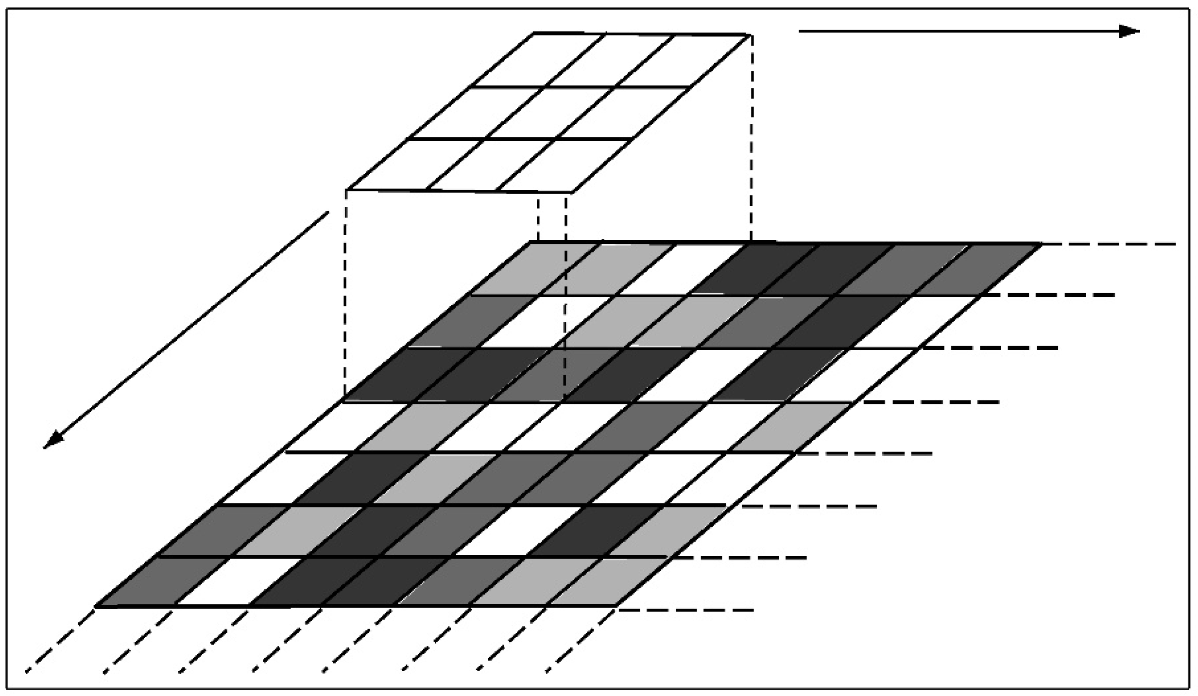
Based on [64,74], spatial convolution filtering is considered as a linear filter for which the brightness value at a certain location in the output image is a function of the weighted average of brightness values located in a particular spatial pattern around the specific location in the input image. This process of the weighted neighboring pixel value is called two–dimensional convolution filtering. This procedure is utilized for the spatial frequency of an image, for instance, high-frequency linear filtering may sharpen the edges in an image, while low-frequency linear spatial filtering is used to reduce noise within an image.
Considering the literature [29,60,64,75,76,77,78,79], four types of spatial convolution filters are common to be used for manual or automated lineament detection: (a) Low pass filter, (b) High pass filter, (c) Linear edge detection, and (d) Non-linear edge detection.
Low-Pass Filtering
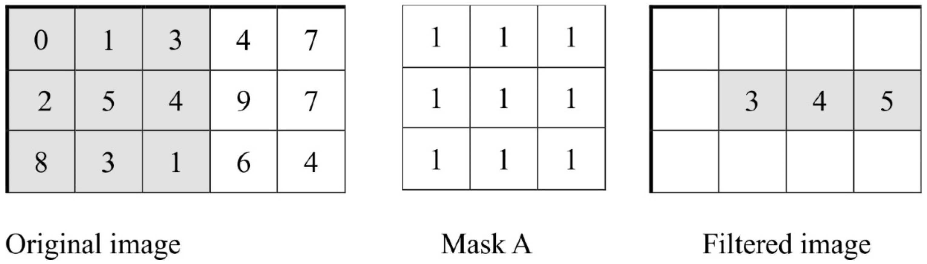
The types of image enhancement that reduce an image’s high spatial frequency are called low frequency or low pass filters [64,80,81]. These filters are useful for removing the noise in the images [64,82,83]. The simple low pass filter assesses a specific input pixel brightness value and the pixels surrounding the input pixel and outputs a new brightness value that is the mean of this convolution [64,84]. The size of the neighborhood convolution mask or kernel is usually 3 × 3, 5 × 5, 7 × 7, or 9 × 9. A typical example is shown in (Figure 1). Jensen [64] states that the coefficients in a low-frequency convolution mask are usually set equal to 1. The calculation of the low pass filter is done using the equation below.
where Ci is the coefficient, Vi is the individual pixel value, and n is the number of pixel covered by the convolution mask.
The filtered image in (Figure 2) is calculated based on the above equations:
The new values in the filtered image:
3 = (0 × 1 + 1 × 1+ 3 × 1 + 2 × 1 + 5 × 1 + 4 × 1 + 8 × 1 + 3 × 1 + 1 × 1)/9
4 = (1 × 1 + 3 × 1 + 4 × 1 + 5 × 1 + 4 × 1 + 9 × 1 + 3 × 1 + 1 × 1 + 6 × 1)/9
5 = (3 × 1 + 4 × 1 + 7 × 1 + 4 × 1 + 9 × 1 + 7 × 1 + 1 × 1 + 6 × 1 + 4 × 4)/9
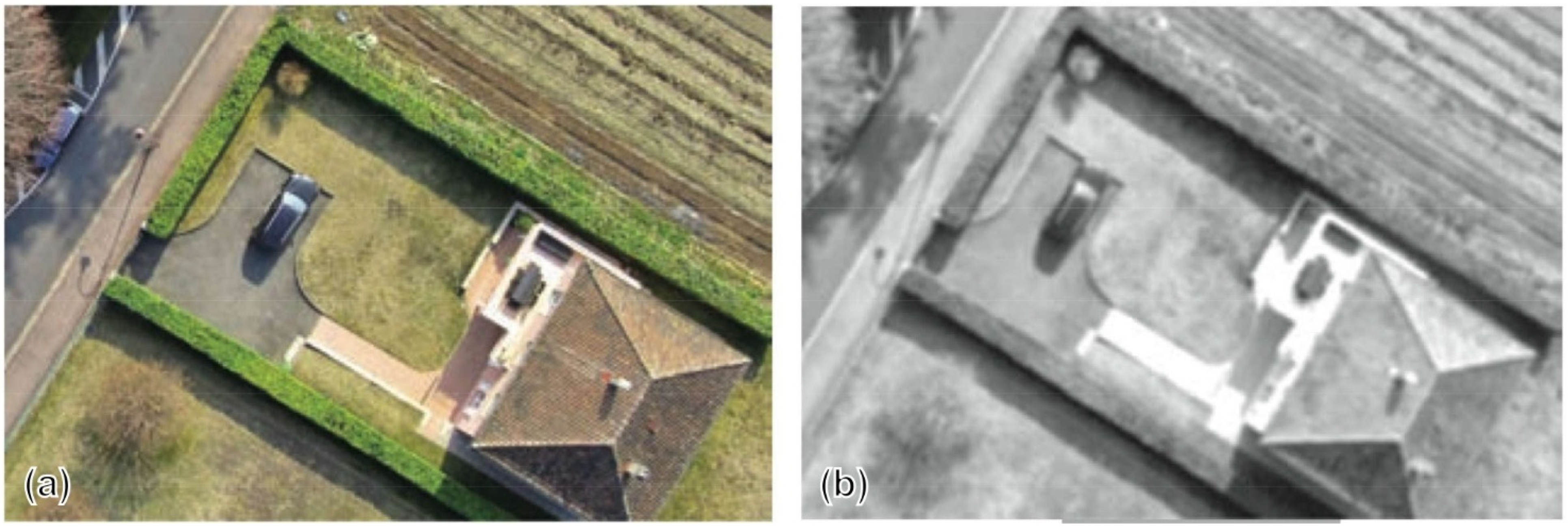
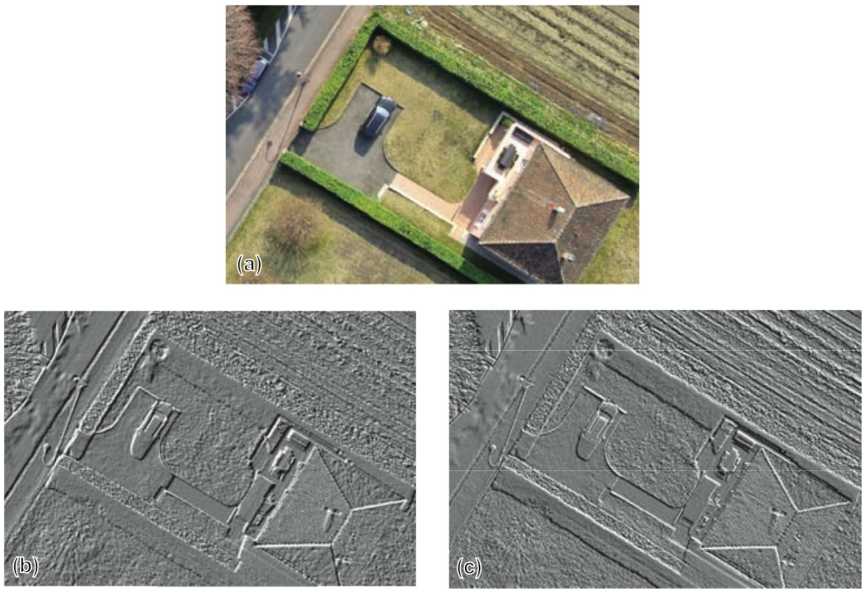
It is notable that low pass filters are used less for the manual extraction of lineaments because the output image is only reduced in terms of noise, and the intensity of blurring is high which causes confusion in lineament extraction. Figure 3 illustrates a visual example of a low pass filtering operation on an original image from a residential area in Germany taken by an unmanned aerial vehicle (UAV) derived from [64]. Figure 3a is a normal color image, while Figure 3b is the low pass filtered image that has been applied on the red band of the original image. In the example, the image becomes blurred by suppressing the high-frequency image.
High-Pass Filtering
High-pass filtering is applied to emphasize or increase the high-frequency components of an image whereas it decreases the low-frequency components. Simply, high-pass filtering is calculated by subtracting the low-pass filter (LPF) from twice the value of the original central pixel value [64,84]:
where BV is brightness value.
Based on [64], due to the high correlation of brightness value with a nine element in high-pass filtering, the filtered image will be characterized by the relatively narrow intensity histogram. Furthermore, the standard kernel used in this filter is 3 × 3 with the coefficients below, which results in a sharpening of the edges.
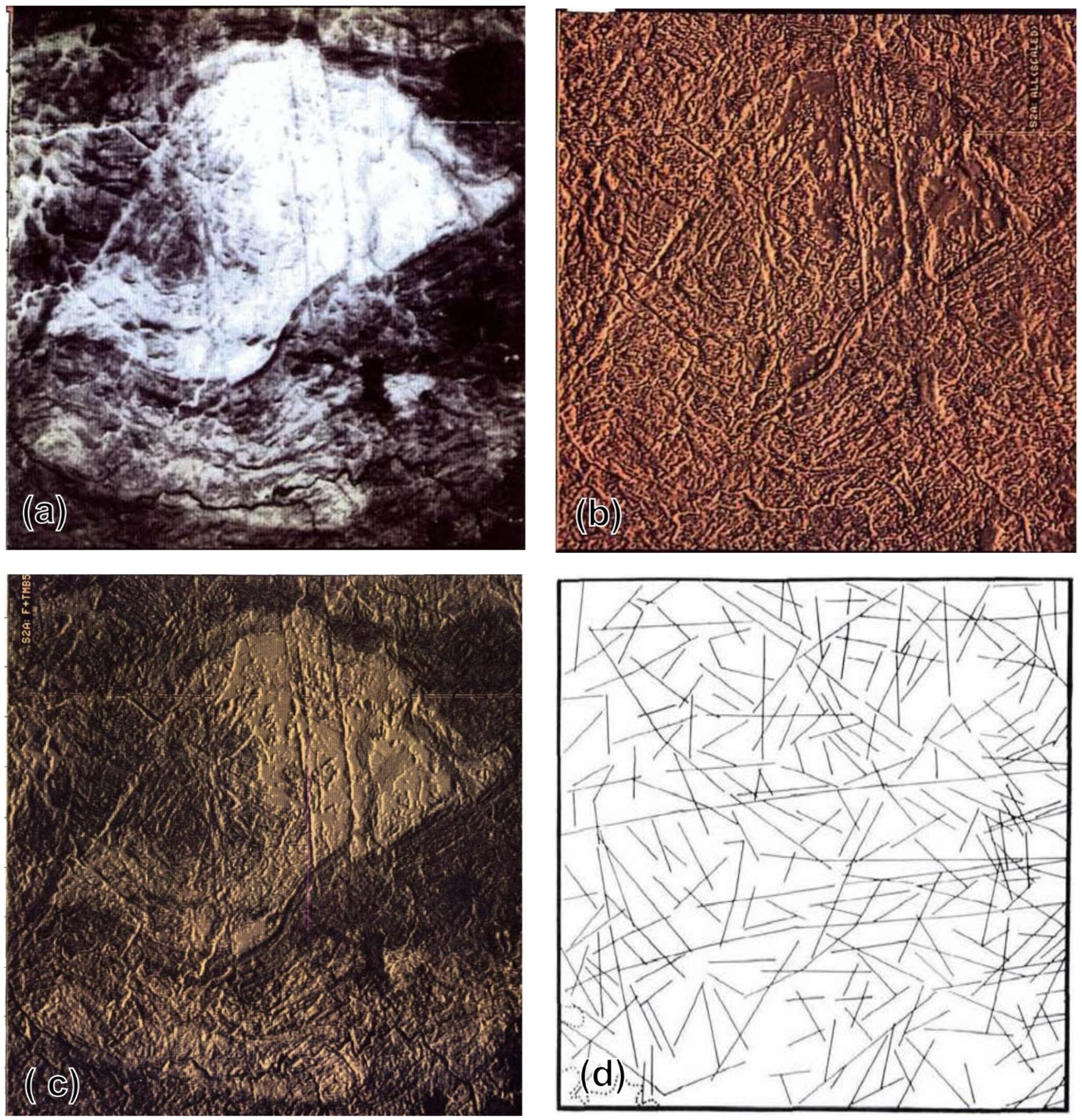
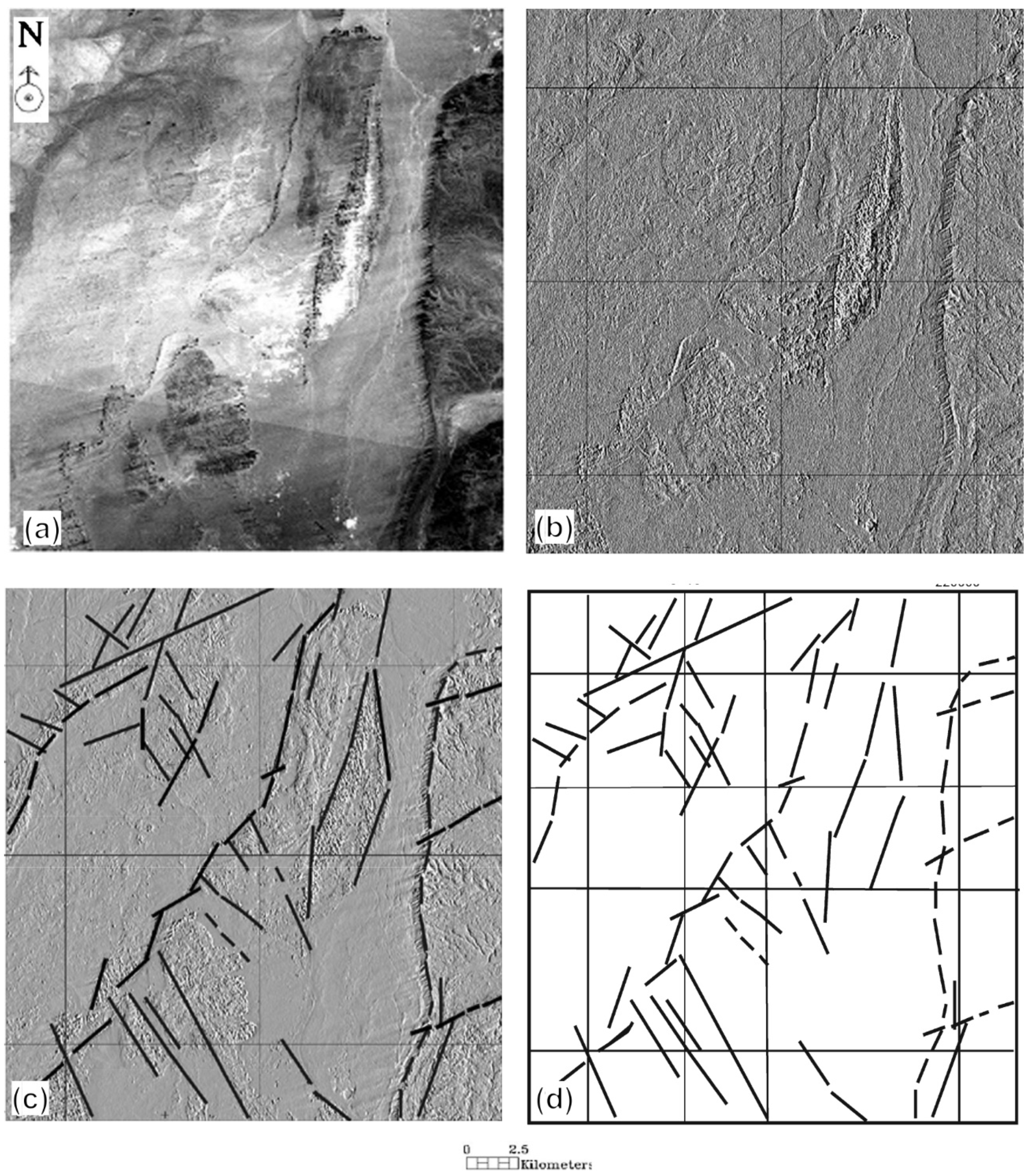
High-pass filtering is commonly used for edge enhancement which increases the chance of lineament extraction using manual interpretation. Typical examples of high-pass filtering using 3 × 3 kernel with different coefficients for the geological lineament extraction are used by [9,29,75]. In these examples, the authors have examined this filtering on Landsat and DEMs over the different areas. Qari [75] examined high pass filtering using a 3 × 3 kernel over the Al-Khabt area, Southern Arabian Shield to manually extract geological lineaments. In this example which is shown in (Figure 4), the author applied the filtering to TM band 5 for edge enhancement to achieve high lineament contrast. Manual extraction of geological lineament from the original image (Figure 4a) seems difficult, hence the image was changed after the filtering was done (Figure 4b). The image became sharp and the features can be clearly highlighted. For better visualization, the author superimposed the filtered image on the TM band 5 (Figure 4c), consequently, the existing lineaments were achieved using manual digitization (Figure 4d).
Linear Edge Detection Filtering
Usually, edges in an image are sharp changes in brightness value between two adjacent pixels [85]. One of the most common methods in remote sensing for geological lineament extraction is edge detection. This can be achieved by the edge enhancement techniques, making the shapes and details more apparent and more convenient to analyze [64]. Based on [85], the human eye considers a sharp and distinctive line between adjacent regions of a picture, but the presence of noise and coarse resolution results in a blur and decreases the chance of appearing of edges. Therefore, edge enhancement techniques are applied to overcome this visual distinctiveness. The edges of remotely–sensed data with a gray value and which change sharply are a significant clue for the delineation and extraction of lineaments [86,87,88].
Like the previous filters, linear detection filtering is usually applied using a particular convolution weighted mask or kernel. One of the most effective linear enhancement filtering techniques causing the edges to appear as a plastic shaded-relief format is emboss filters. The edges are obtained using emboss east and emboss northwest directions with the coefficient below [64]:
Compass gradient masks are another type of linear edge detection filtering which is used for discrete differentiation directional edge enhancement. The Compass filter uses eight different commonly gradient mask directions (N, E, S, W, NE, SE, SW, NW) [64,89]. The different direction masks with their associated coefficients are shown in (Table 2).
Jensen [64] examined typical examples of Emboss and Compass filters on the red band of the original color image with high spatial resolution of a residential area in Germany (Figure 5a). Jensen applied Emboss Northwest filtering to achieve the plastic shaded-relief for better visualization of edges (Figure 5b). Figure 5c illustrates the Compass Northeast filtering of the original image.
Another four 3 × 3 alternative directional filters have been proposed by [73] for edge detection with their associated coefficient, as below:
The last linear edge detection filtering is referred to as Laplacian filtering, applied to imagery to perform edge enhancement. This filtering is a second derivative edge enhancement filter without regard to edge direction [64]. The 3 × 3 Laplacian filters are described as below with their coefficients:
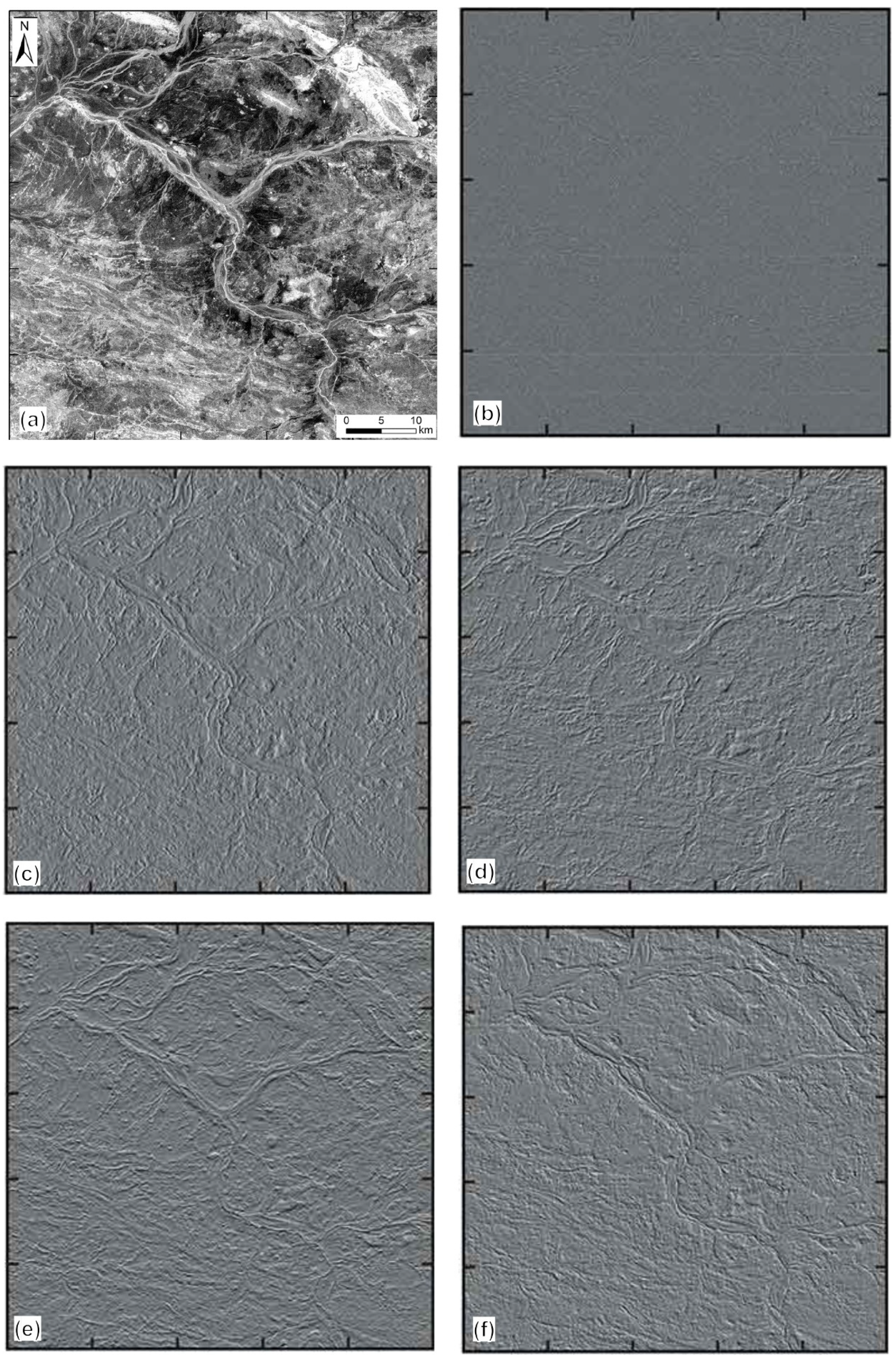
Linear edge enhancement filtering has been widely used for geological lineaments over the last few decades [76,79,90]. For instance, Farahbaksh [79] tested image transformation and enhancement to extract geological lineaments over the Yinnietharra area, Western Australia using Landsat 8 OLI/TIRS data. Farahbakhsh selected the output of Minimum Noise Fraction (MNF) with the highest eigenvalue to apply the Laplacian and directional filtering (Figure 6). As a result, almost all linear features, including geological lineaments and streams, can readily be extracted from the filtered images. The findings of [79] show that directional filtering has more effective results in the different striking of geological lineaments (Figure 6c–f), while the Laplacian filtering failed in detecting particular strike (NW–SE) lineaments (Figure 6b).
Nonlinear Edge Detection Filtering
The non-linear edge enhancement filtering is based on the non-linear combination of pixels. The most common types of this filtering are the Sobel filter, Prewitt filter, and Robert filter [64,73,91,92].
Sobel edge detection filter is followed by the 3 × 3 window numbering and is calculated using the following equation:
where
And V is the individual pixel value.
Sobel kernels are calculated in four principal directions (N–S, NE–SW, E–W, and NW–SE) and are applied in a single band, particularly band 7 of ETM+ due to the greater wavelength and lesser effect of moisture due to the minimal effect of atmospheric haze [59,60,70]. The associated coefficient in four directions is shown in (Table 3) [93,94,95,96].
An example of the capability of Sobel filtering for automatic geological lineaments was carried out within the Ikole/Kabba region, southern Nigeria by [94] (Figure 7). In this example, Salawu et al. examined Sobel directional filters mainly in the four directions: N–S (Figure 7b), NW-SE (Figure 7c), NE–SW (Figure 7d), and E–W (Figure 7e), on the band 8 image of Landsat 8 OLI/TIRS. A 3 × 3 convolution mask was used in this example in which the results are promising in terms of linear features. The authors extracted the lineaments for each filtered image corresponding to distinct directions, then integrated all the extracted lineaments with the geophysical and field work data.
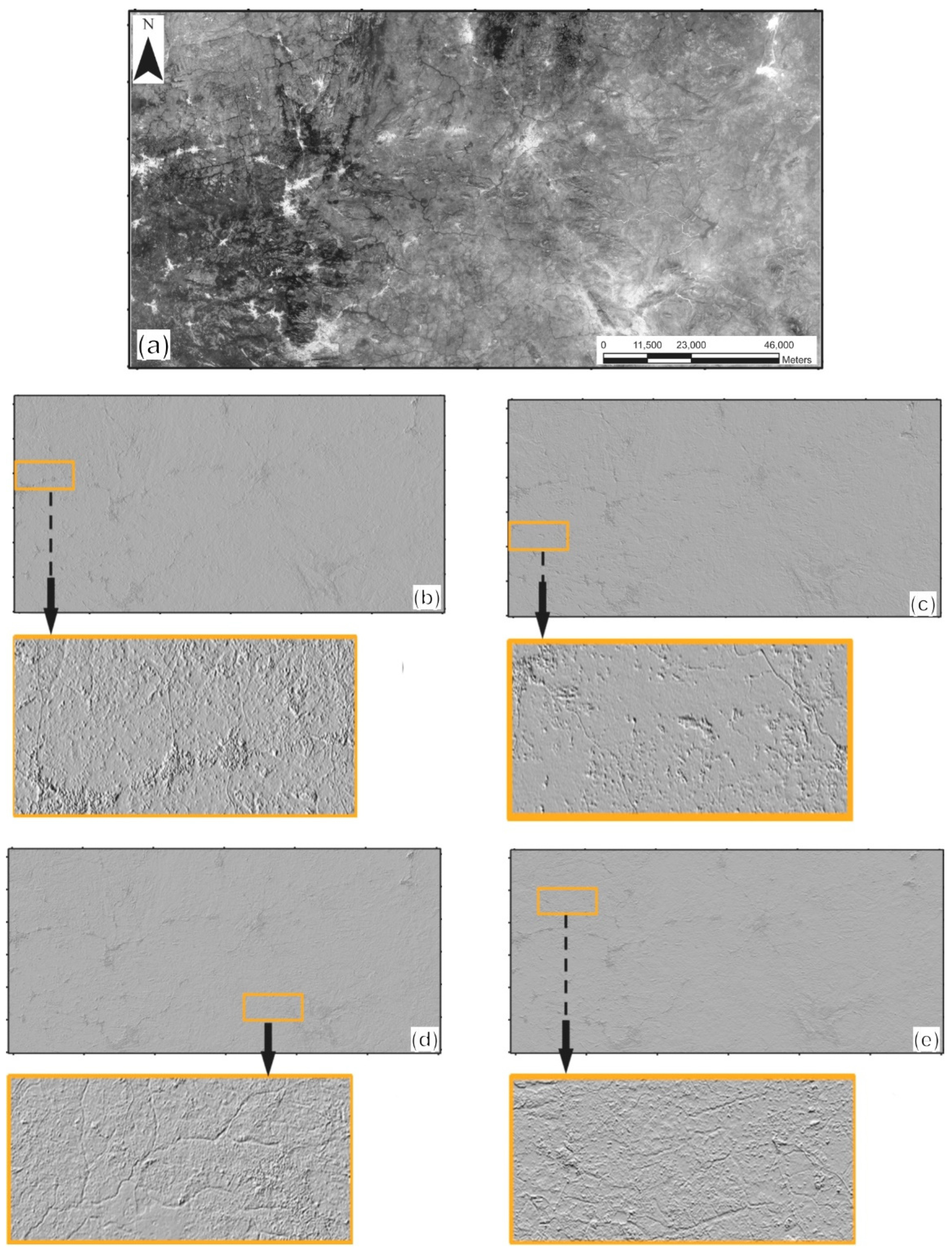
The Prewitt filtering for edge detection contains two groups of 3 × 3 windows, including horizontal and vertical; however, the edges and lineaments in most cases have more than two directions. Therefore, to detect more direction edges, a Prewitt filtering window of six or eight is utilized (Table 3) [97,98]. The Prewitt filtering is more clarified in the study conducted by [98]. Boutrika et al. [98] applied Prewitt filtering on Landsat 7 ETM+ to extract geological lineaments associated with gold mineralization over the Central Hoggar, South Algeria. In this work, Boutrika et al. performed Principal Component Analysis (PCA) on a multispectral band, and then applied Prewitt filtering using a 3 × 3 convolution kernel on PC1 in four directions (N-S, NE-SE, E-W, and NW-SE) (Figure 8). The structures can clearly be distinguished in (Figure 8b), obtained from the overlaying four direction filtered images. The authors highlighted the geological lineaments corresponding to the deep faults on the filtered image (Figure 8c), in which the extracted lineaments are illustrated (Figure 8d).
The Robert edge detection filtering is performed by a simple, quick, two-dimension spatial gradient measurement on an image. Once this filtering operation is done, the high spatial frequency regions corresponding to edges are highlighted in the image. Robert is using 2 × 2 mask convolution to give edges in x-direction and y-direction, respectively [99,100,101].
A typical example of Robert filtering applied on the red band of high spatial resolution color image of a residential area, Germany was carried out by [64] (Figure 9a,b).
The directional and nondirectional filtering is applied for lineament extraction at various scales and disciplines. The results achieved by them are diverse. In terms of geological lineament extraction, directional filtering has more effective results because faults and fractures are usually distributed at different strikes. Therefore, filtering in a particular direction may not give a suitable product. Several studies are concerned about the directional filters for geological lineaments, e.g., [76] tested directional (Sobel) and nondirectional (Laplacian) filters on the particular bands of Landsat ETM and claims that directional filters in NE-SW and NW-SE gave the best results because the prevailing tectonic trends were at the NE-SW and the NW-SE directions considering the tectonic regime of the study area.
Pour & Hashim [35] applied 7 × 7 user-defined directional filtering in the central gold belt, Peninsular Malaysia on PALSAR data to map the lineaments with their specific trends. Four lineaments in total, trending N-S, NE-SW, NNW-SSE, and ESE-WNW, were determined, which are compatible with the ground truth studies and the previously mapped faults.
Allou et al. [77] mapped the faults using different directional filters over an area in western Africa. He applied 7 × 7 convolution of Sobel, Prewitt, and Yesou filters in three major directions (N-S to NNE-SSE, N90o to N100o, NW-SE to NNW-SSE); the authors stated that the high density of lineament had been detected using Prewitt filters on panchromatic bands, while the less dense is detectable by Yesou filters. Further works on lineament extraction using directional and nondirectional filters are stated in (Table A1).
2.1.3. Multiband Analysis
The usage of multiband analysis of remote sensing data plays a critical role in the determination of lineaments. Multiband analysis of remote sensing imageries is mostly applied in visual interpretation or manual lineament extraction of geological lineaments. This analysis is impressive when it is integrated with other outputs of enhancement or filtering. The most applied multiband analysis in lineament delineation through photo interpretation are Principal Component Analysis (PCA), False Color Composite (FCC), and Band Ratio (BR).
Principal Component Analysis (PCA)
Principle component analysis is a multivariate statistical technique to reduce the data dimensionality by transforming the selected data into a new principal component axis, generating an uncorrelated image that contains higher contrast than the original bands [102,103]. According to [64], PCA is the spectral enhancement technique of an image by compressing the information of several spectral bands into just two or three transformed principal component images. Singh & Harrison [104] states that new principal component images may be more interpretable than the original data as the multispectral dataset’s dimensionality is reduced. Furthermore, the newly generated PCA images have more spectral difference, and the existing objects can be extracted effectively. PCA is more applicable for lithological mapping, and each lithological unit is revealed clearly in PC images; based on the selected minerals, the PC is selected, or sometimes, the composition of several PCs is created. The boundary between two adjacent lithologies may be considered a lineament or sometimes a fault. Therefore, the analyst can easily digitize the edges from PC images.
PCA is mostly used as a supportive method; for instance, [70], in a study, used PCA as multiband analysis to support the results of directional filters for geological lineaments. In this study, band 7 of Landsat TM was used for spatial filtering, and then PCA improved the image. The authors meant to transfer all the spectral information into three bands; after the calculations, the information was accumulated into the three first bands (96.31%). This could help the authors better to interpret the color composites of these three PCs visually. The result of the lineament map by PC composite interpretation shows about a 17% increase with a concentration in a particular direction which causes authors to take the directional filtering into account.
Novak & Soulakellis [28] examined PCA analysis for geomorphic features on Landsat 5 TM over an area in Greece. He visually interpreted the two sets of PCs (PC1, PC2, PC3) and (PC4, PC5, PC6), respectively. 97% of information belongs to the first set. Furthermore, he composed the Red and SWIR-2 with the first two PCs as a false color composite for better visualization. The lineaments detected by this manual method were correlated to the previously mapped faults and were considered new faults, tectonic and lithological contacts. Another study by [90] reveals the PCA method’s capability in manual geological lineament extraction using Landsat 5 TM in western Turkey. The author generated the principal component of all six multispectral bands and then found the most loaded PC; finally, he composed three highly loaded PC images to digitize the lineaments. Lastly, the author integrated the results from PCA with the results obtained by edge enhancement filtering. Several similar studies have been conducted, aiming at geological lineament extraction using PCA along with other spatial and spectral enhancement methods, e.g., [79,105,106].
False Color Composite (FCC)
The band combination or color composite is composed of the three various bands in red, green, and blue (RGB) order; if the composed bands are red, green, and blue, the combination is called true color combination as every object is displayed in its natural color. In contrast, the false color combination is the composition of electromagnetic spectrum channels as red, green, and blue (RGB). The resultant image of the object is not visualized in its natural color [107,108,109]. The Optimum Index Factor (OIF) procedure was devised by [110] to rank all the possible combinations of triplets within a given set of spectral bands in order of statistical information contents. In other words, it is the procedure of selection of the best combination of spectral bands for subsequent false color composite. The suitable selection of band composite is also performed using deterministic methods based on the consideration of the targeted objects’ spectral characteristics.
Salvi [111] applied false color composite on Landsat TM over Central Italy to interpret the existing geological faults and lineaments. The author utilized the OIF procedure on six VNIR bands to select the best band composite. The OIF ranking result shows that the composition of bands 5, 4, and 1 are suitable to differentiate the objects on the image.
According to [60], false color composite increases the interpretability of the data for manual lineament extraction; among the composites, the author states that the best visual quality is achieved with a false color composite of visible and near IR bands. Therefore, the combination of 432 as red, green, and blue, respectively, for Landsat ETM, was used to identify the linear patterns of vegetations, geologic formation boundary, river channels, and geologic weakness zones.
Band Rationing (BR)
Band rationing is the division of one spectral band by another, based on the spectral characteristics of selected objects. Sometimes similar targeted surficial objects produce different brightness values due to topographic slope and aspect, shadows, or seasonal changes in sunlight illumination angles and density in single or multiple bands, which may confuse the interpreter. Band rationing techniques transform the data, reduce the environmental effects, and provide information that may not be available within a single band [64,112]. BR is calculated as:
where is the output for a pixel at row i and column j; is the brightness value in band k at the same location and is the brightness value in band l.
According to [113], several band ratios which are combined in RGB offer greater contrast between the units than the individual band false color images. Furthermore, sometimes band combinations are made of three band ratios for better visualization.
Sarp [60] tested a band ratio of 5/7 in Landsat ETM to remove the effect of shadows, aiming to detect and interpret linear features easily. In most cases, lineament may be the boundary of two adjacent lithologies. Therefore, the author examined three band ratios (5/7, 2/3, 4/5) as an RGB combination to improve visualization in the manual lineament extraction process. The logic behind selecting these band ratios is: 5/7 discriminates the hydroxyl bearing minerals as a good indicator for the water effects along the fracture, 2/3 delineates the contrast between dense and sparse vegetation, and 4/5 highlights the distributed areas in a dark or black tone. Most of the works associated with lineament extraction using multiband analysis during the last few decades are shown (Table A1).
2.2. Semi-Automated Lineament Extraction
Semi-automated lineament extraction is the process of lineament detection based on some digital image analysis techniques and visual interpretation. Once the pre-processing and enhancement are performed, the lineaments are extracted using digital image analysis and somehow the manual editing of detected lineaments is also conducted by the user [6,62,70,114]. Concerning manual lineament extraction approaches, this method takes less time and achieves the result faster; however, it may mix the artifact lineament in the resultant map. According to [115]’s statement, semi-automated lineament detection produces more structure than human interpretation, as image processing might be better to enhance the subjected image and linear features. In total, five steps are included in semi-automated lineament extraction: pre-processing, edge detection, edge tracking, edge linking, and vectorization [116]. A bit of enhancement and filtering operations are carried out before the image processing; the enhancement and filtering techniques have been discussed in the previous section. Once the pre-processing is completed, different algorithms, including object-based classification, segmentation, segment tracing algorithm (STA), Hough Transform, and PCI Line, are applied [116,117,118]. Those works which have been done using the semi-automated method are stated in (Table A1).
Mallast et al. [117] have applied semi-automated lineament extraction, combining linear filtering and object-based classification on DEM to delineate the lineaments over the Dead Sea in Israel. The authors operated the 30 × 30 matrix filter and other 5 × 5 s-order filters in four directions to enhance linear features’ appearance. Then, they ran the object-based classification on the generated map using segmentation and vectorization. For a better generation of lineament maps, the authors combined the resultant lineament with the automated lineament extraction Canny algorithms; also, they used ancillary data such as geology and drainages to differentiate the significant lineaments from insignificant. Lastly, the author concluded that medium resolution DEM is sufficient data for lineament extraction if it is followed by the auxiliary data and highlighted the capability of semi-automated lineament extraction.
A novel study by [119] shows the capability of the semi-automated method using Unmanned Aerial Vehicles (UAVs) for the mapping of geological structures (faults, fractures, and joints). The authors first detected the geological structures over a small area in the 2D environment, then transferred them into a 3D model to calculate the dip and dip direction. 79.8% accuracy of semi-automated methods is reported compared to expert manual digitizing and interpretation methods. Furthermore, the authors estimated that time is reduced from 7 h to 10 min when the geological structures are mapped using the semi-automated method instead of the manual method.
Semi-automated tectonic structure mapping has been applied in a research by [120]. The author developed a semi-automated method by using software “CurvaTool” and user thresholding. Digital Terrain Model (DTM) has been utilized in this study. The author called this methodology semi-automated because two threshold values are asked from the user, including the expected orientation of data sets of lineaments and their variability range. After the edges are extracted, manual editing may be required to achieve a complete and correct set of lineaments. The results achieved by this developed software were compared with literature data for validation, and good correspondence between literature data and CurvaTool was found concerning the geometry and distribution of the lineaments.
A recent work by [118] highlights the objectivity of semi-automated lineament extraction using Object-Based Image Analysis (OBIA) with high-resolution remote sensing and airborne geophysical datasets. The Southwest of England was tested for this analysis. Here two complementary methods (top-down and bottom-up) segmentations were applied using Trimble eCognition software. The results from the two methods are the same. The results were validated by the data obtained during the survey and field works.
2.3. Automated Lineament Extraction
Automated lineament extraction is performed using computer-assisted software. The automated processing includes enhancement, filtering, edge detection, and finally, lineament extraction. There are several algorithms developed by scientists which automatically extract the lineaments, e.g., Hough Transform [23], Lineament Extraction and Stripe Statistical Analysis (LESSA) [121], Segment Tracing Algorithm (STA) [62], Canny Algorithm [69], ADALGEO [122], TecLines [123], Lineament Detection and Analysis (LINDA) [124]. These algorithms are designed to operate via a software package and give the final lineament map in vector format. An automated lineament extraction algorithm takes into consideration the noise, threshold, size, and orientation of linear features [125].
The automated lineament extraction methods help the analyst to produce the result in a short time; however, they still will contain some problems. Sometimes the extracted lineaments or linear features do not correspond to geological structures. Therefore, the user or analyst is obliged to evaluate the extracted lineaments or integrate the manual interpretations.
Many considerable works on geological faults and lineament detection exist which use automated algorithms for diverse remote sensing data, e.g., Landsat MSS [12,80], Landsat ETM+, OLI [59,76], ASTER [122], DEM [45,115], Radar data [34,126], high spatial resolution data IKONOS [84] (Table A1).
The earliest automated lineament extraction is the application of Hough transform; a technique being used to separate specific shape features in an image. The algorithm is commonly used for the detection of lines, circles, and ellipses [60]. The Hough transform was firstly applied by [23] for the detection of straight lines representing geological lineaments over an area in Sudbury in Canada. The author stated that being relatively unaffected by gaps in lines and by noise are the main advantages of Hough transform algorithm. The procedures involved in this study are finding local maxima, application of an inverse Hough transform, and straight-line profile analysis. Firstly the author pre-processed the image using a 3 × 3 median filter, and an algorithm was applied to trace all the edges in the image; then, Hough transform was applied to the edge image to produce the cumulator arrays where the brighter tones represented higher counts. Once the local maxima was selected, the inverse Hough transform, and straight-line profile analysis were done to obtain the lineaments.
Vassilas et al. [11] also applied the automated lineament extraction using the Hough transform algorithm; however, the algorithm was modified. The authors first performed data clustering using a self-organizing map, then binarized the classification, and finally applied the modified Hough transform in order to identify lineaments around the Vermion area in Greece. Another study by [45] also shows a Hough transform automated lineament extraction algorithm. In this study, the author tested three spatial data JERS-SAR, Landsat TM, and DEM, for automated and manual interpretation. The final lineament map was obtained using the pre-processing, filtered image in binary format, and finally, the Hough transform algorithm application.
Another developed automated lineament extraction algorithm is the Segment Tracing Algorithm (STA) by [62]. This algorithm was commonly used before the year 2010 for the purpose of geological lineament detection. The STA principle is to delineate a line of pixels as vector elements by examining local variance of the gray level in digital images and connecting the line elements along with their expected directions. In a study, Koike et al. [62] described that the advantages of the proposed algorithm over usual filtering methods are its capability to trace only continuous valleys and extract more lineaments parallel to the sun’s azimuth and those located in shadow areas.
Masoud & Koike [126] performed an updated application of STA to automatically delineate tectonically significant lineaments with SRTM DEM and geophysical data. In this study, the authors used 30 arc-second DEM, 1-min gravity anomaly girds, and 2-min total field magnetic intensity grids covering Egypt. Using the developed techniques, orientations, and styles of faulting (normal, reverse, and strike-slip types) were detected.
Development in programming languages has also promoted the creation of self-programmed software regarding the automated geological lineament. One of them is TecLines, a MATLAB-based toolbox developed by [123]. In this toolbox, the authors have integrated several functions e.g., filters in both frequency and spatial domains, tensor voting framework to produce binary edge maps, and the Hough transform algorithm to extract linear image discontinuities; also B-spline as polynomial curve fitting was used to eliminate the artificial line segments, which are out of interest. The results have been compared with Canny and other algorithms, which give considerable results. The TecLines toolbox has two parts; Line segment detection and Extraction & Line Linking and Merging, which have been published in two separate works [123,127].
In addition to other algorithms, wight overlay analysis is also considered a suitable automated geological lineament extraction approach. Abdullah et al. [115] examined an overlay model technique to produce a predictive fault potential map. The authors considered four significant factors: drainage patterns, previously mapped faults, lineaments, and lithological contact layers. The layers have been created using various techniques; among them, lineament maps were achieved automatically via band 5 of Landsat ETM −7 using PCI Geomatica software. Then, the layers were weighted considering their importance in terms of faulting. The final resultant map was classified into five potential zones: very low, low, moderate, high, and very high. Lastly, the fault line was extracted and compared to the data obtained from the field; a high correlation is seen between the data, which shows the technique’s capability.
A recent visual basic-based software LiNDA (Lineament Detection and Analysis) was developed by [124]. This software is a graphical user interface that automatically detects and analyzes the linear features from grid data of DEM, gravity, magnetic, and other remote sensing data. This software’s most useful ability is to calculate strike, dip, and estimate the fault type with interactive viewing of lineament geometry. The main working scheme of LINDA includes selection of source grid data, segment detection, and grouping based on STA, transformation from segments to lineaments based on B-Splines, identification of fault type, estimation of strike & dip, construction of fault plane, and the final stage of lineament display with fault type, rose diagram of strikes, and Schmidt’s net of directional frequency [124].
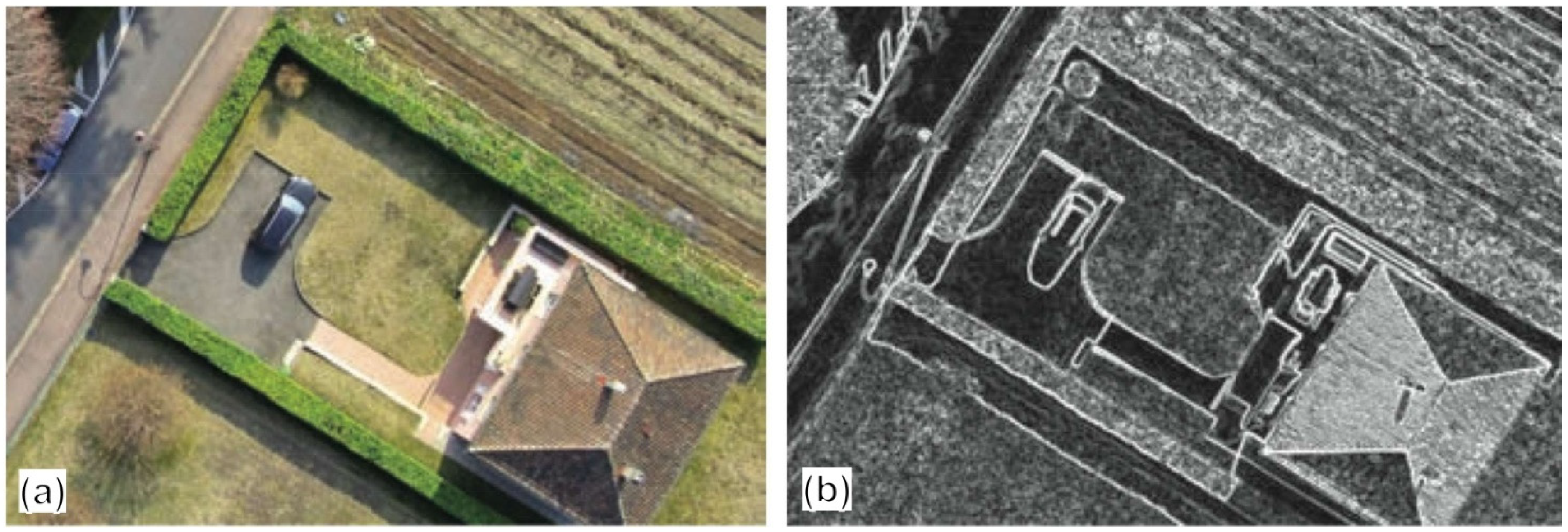
Canny edge detection algorithm is another powerful automated linear feature detection that was developed by [128]. According to this algorithm, image convolution with a Gaussian kernel is performed to smooth noise and computes the edge strength and direction for each pixel in the smoothed image. Canny algorithm is based on computing the gradient magnitude that is above some threshold, identified as edges. In other words, this algorithm is applied to smooth the image and reduce the noise, and then find the image gradient to highlight regions with high spatial derivatives.
Consequently, the algorithm goes through these regions and overthrows the pixels which are not at the maximum. The gradient is still further reduced by hysteresis. Hysteresis is utilized to go along the remaining pixels that have not been overthrown. Hysteresis uses two thresholds. Suppose the magnitude is below the first threshold. In that case, it is marked to zero (made a non-edge); on the contrary, if the magnitude is above the high threshold, it is made to an image. In contrast, if the magnitude is between the two thresholds, then it is set to zero, representing a path from this pixel to a pixel with a gradient above the threshold [69,79,128].
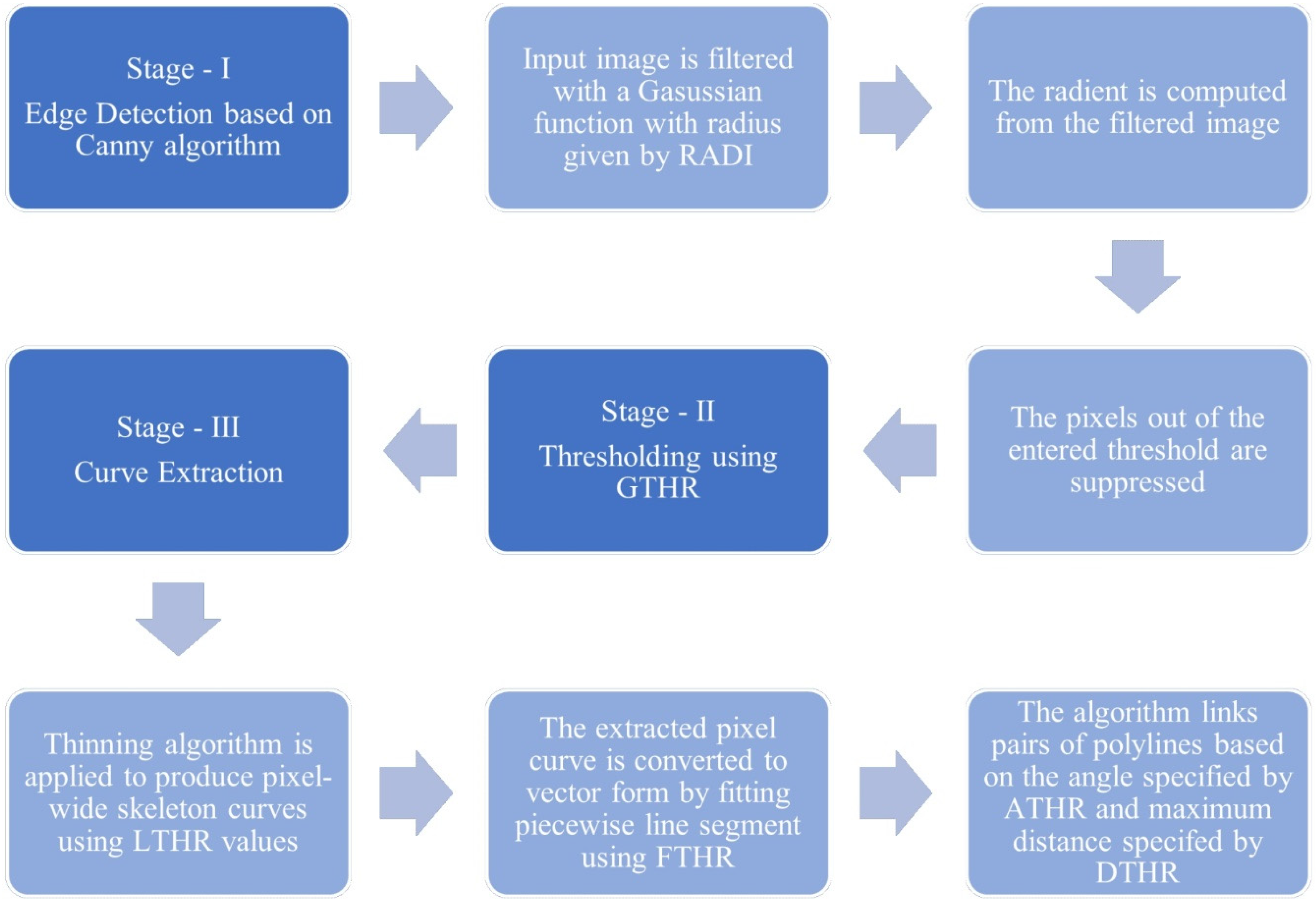
In recent years, LINE module of Geomatica software has become the common tool for automated geological lineament extraction [79,84,129,130,131]. The LINE module’s logic is the same as the STA algorithm; however, it also worked based on the Canny algorithm in the first stage of operation. The LINE module of PCI Geomatica extracts the line features. It gives the output as vector segments by using the six parameters: Filter Radius (RADI) with recommended values between 3–8, Edge Gradient Threshold (GTHR) with accepted values between 10–70, Curve Length Threshold (LTHR) with the common value of 10 in most cases, Line Fitting Error Threshold (FTHR) with the recommended values between 2–5, Angular Difference Threshold (ATHR) with the suitable angle between 3 to 20 degrees, and Linking Distance Threshold (DTHR) with efficient values between 10 to 45 [34]. These parameters are also operated by three stages (in blue), as depicted in (Figure 10).
3. Discussion and Concluding Remarks
During the last few decades, remote sensing has proven its effectiveness in every branch of geology, particularly in structural geology, tectonics, lithological mapping, and earthquake monitoring. Lineament is a geological feature that includes faults, fractures, joints, and lithological boundaries. These structures can predominantly be determined from diverse remote sensing data sources and techniques. As such, the determination of geological lineaments allows the sufficient exploration of mineral deposits associated with hydrothermal alterations and magmatic processes. In addition, the lineaments can act as the influencing factors of groundwater potentiality, natural hazard assessment, including earthquakes and seismicity, and land sliding.
Conventional geological lineament methodology is time-consuming and expensive. On the other hand, conventional approaches are challenging to apply due to the physical/geographical condition of the region of study. Remotely sensed mapping of geological lineaments leads to determine the faults, and their tectonic implication is the substitution of conventional methods. Manual geological extraction is carried out on the computer screen or hard copies. The growth of technology has changed the photo interpretation operation from the early usage of the stereoscope and transparent overlays to a very fast computer screen with HD displays. Manual geological lineament extraction is directly associated with the interpreter’s skill and experience and the remote sensing data. As the lineaments, the sharp and distinctive line between adjacent regions of an image, are seen by human eyes, therefore, an image with coarse resolution and noise resulting blur decreasing the chance of appearing edges and/or linear features. To overcome this visual distinctiveness, different edge enhancement and filtering are applied. Ramli et al. [31] stated the manual lineament extraction subjectivity as a controversial result, reproductivity, and positioning in highly vegetated or wide valleys. The authors also described the final lineament map as integrated with the results from multiple observers to minimize the subjectivity.
Automated and semi-automated approaches of the lineament extraction are performed using computer-assisted software, which is considered one of this approach’s main objectivities. The results of the automated and semi-automated techniques depend on the remote sensing data and the algorithm to be applied. The remote sensing data are varying regarding the contrast and the resolution. Therefore, various edge enhancement, directional, and nondirectional filtering are applied to data before the extraction algorithm’s operation. STA, Hough Transform, LINDA, Curvatool, and TecLines are the standard algorithm which are utilized for the determination of geological lineaments. Extraction of lineaments is an easy task using automated algorithms. However, in most situations, the algorithm generates segmented images containing several spurious lineament pixels that are not corresponding to geological lineaments. Ramli et al. [31] consider this issue as the main problem with automatic lineament extraction caused by the filtering.
Furthermore, the automatic algorithms cannot effectively map the geological lineaments from low-contrast and mountain shadows, resulting in a low density of lineaments [62]. To overcome this problem, Koike et al. [62] proposed the STA non-filtering method, which extracts the lineaments based on the entered thresholds. Currently, the LINE module in PCI Geomatica software is widely used for the lineament extraction, which is based on the STA and Canny algorithms.
The reviewed literature shows that automated and semi-automated techniques have been applied to detect most works’ geological lineaments. The author’s experience and review of the previous literature results disclose that a single technique may not efficiently determine the exact geological lineaments excluding artifacts. Therefore, it is suggested to generate a significantly tectonic–geological lineament map using the integration of automatic and manual techniques. The generated map should be compared and verified with the previously every possible mapped structure. In case of possibilities, integration of geophysical data and extensive fieldworks is suggested. Geological lineaments are extracted for various purposes such as tectonic faults, hydrogeology, urban studies, earthquakes. In each case, specific validation and accuracy assessment is applied. In targeting the tectonic faults, the generated geological faults are validated using paleoseismic data or previously mapped faults. The generated map is suggested to be validated with the land deformation deduced by the seismic activities to get the confidential result. The seismic activity or land deformation must indicate an active fault. Therefore, geological lineaments’ distribution might be observed in an area with high activity of seismicity and land deformation. Assessment of land deformation around the detected lineaments is performed using GPS stations, conventional geological methods, and remote sensing data. Radar data, particularly Interferometric Synthetic Aperture Radar (InSAR), can effectively produce the land deformation assessment maps showing uplift and land subsidence with their associated velocity.
Author Contributions
H.A. contributed the main conceptualization, designed the methodology, investigated literature, analyzed data, wrote the first draft of the manuscript. E.P. supervised the data analysis, draft preparation, review, and edited the manuscript. All authors have read and agreed to the published version of the manuscript.
Funding
This research received no external funding.
Acknowledgments
The authors thank Kerem Pekkan for his constructive comments and suggestions that have developed the manuscript. Also, two anonymous reviewers are thanked for their thoughtful comments and suggestions that helped enrich this work.
Conflicts of Interest
The authors declare no conflict of interest.
Appendix A

Table A1.
Geological lineament detection using various techniques between 1975 to 2021.
| No | Date | Method | Data | Place | Reference |
|---|---|---|---|---|---|
| 1 | 1975 | Manual lineament extraction including high-pass filtering Computer-aided automated lineament extraction | Landsat 1 | Anadarko basin, Oklahoma, and Colorado Plateau | [29] |
| 2 | 1985 | Automated lineament extraction using an algorithm based on the maximum local brightness gradient | Landsat MSS | Cevennes, Southern France | [21] |
| 3 | 1986 | Geological lineament extraction using visual interpretation | Landsat MSS | Western England | [132] |
| 4 | 1989 | Automated lineament extraction following enhancement filter | Landsat 1 | Tamilnadu state, India | [125] |
| 5 | 1990 | Automated lineament mapping using Hough Transform | Landsat TM | Sudbury, Canada | [23] |
| 6 | 1991 | Manual lineament structures mapping using edge enhancement by high pass filtering in band 5 | Landsat TM | Al-Khabt Area, Southern Arabian Shield | [75] |
| 7 | 1992 | Automated lineament extraction using LESSA (Lineament Extraction and Stripe Statistical Analysis) | Landsat TM | Moscow Russia | [121] |
| 8 | 1995 | Automated lineament analysis using Segment Tracing Algorithm (STA) | Landsat TM and DEM | Japan | [62] |
| 9 | 1995 | Visual interpretation using OIF, FCC | Landsat TM | Abruzzi region Central Italy | [111] |
| 10 | 1998 | Manual lineament extraction using band combination Automated lineament extraction | Landsat TM | Ebro Basin NE Spain | [133] |
| 11 | 1998 | Manual geological lineament extraction using histogram equalization and stretching, PCA, Prewitt, and Sobel filters | Landsat TM | Central Turkey | [70] |
| 12 | 2000 | Geomorphic features detection by visual interpretation using PCA and FCC | Landsat TM | Lesvos Greece | [28] |
| 13 | 2001 | Automated lineament extraction using the SWIR bands and GeoAnalysis PCI EASI/PACE | Landsat TM | Natash area Egypt | [134] |
| 14 | 2001 | Manual interpretation for delineation of tectonic features | Landsat ETM | Northern half of Arabian Shield | [135] |
| 15 | 2002 | Automated lineament extraction using Hough transform | Landsat TM | Vermion Greece | [11] |
| 16 | 2002 | Automated lineament extraction using Hough transform | Landsat TM, JERS-1 SAR, DEM | Kyungsang basin, Korea | [45] |
| 17 | 2003 | Visual Interpretation using band 4 of Landsat 4 and 234 of IRS | Landsat 4 MSS, IRS LISS-I | Pranhita-Godavari basin, India | [136] |
| 18 | 2003 | Manual lineament extraction using Weighted Moving Average (WMA) for fracture pattern determination | Landsat TM | Coastal Cordillera, Northern Chile | [137] |
| 19 | 2003 | Manual lineament extraction using Laplacian, Ford, Sobel, Kirch, and directional filters. Automated lineament extraction using Canny multi-scale edge detector was applied for verification | Landsat 7 ETM+ | Alevrada, Central Greece | [76] |
| 20 | 2004 | Manual lineament extraction using visual interpretation of anaglyph images for fault system and geomorphological feature detection | Landsat TM, ASTER, DEM | SW Turkey | [58] |
| 21 | 2004 | Manual lineament extracting using FCC, PCA, edge detection filters | Landsat 5–TM | Bakircay plain, western Turkey | [90] |
| 22 | 2004 | Active fault mapping using visual interpretation | ASTER | Bam, SE Iran | [27] |
| 23 | 2004 | Discontinuity mapping using automated lineament extraction in LINE module of PCI Geomatica | IKONOS | Golbasi, Ankara, Turkey | [84] |
| 24 | 2005 | Automated lineament extraction and analysis after fusion using LINE module of PCI Geomatica | Landsat ETM+, ASTER | Suoimuoi catchment, Vietnam | [138] |
| 25 | 2005 | Morphotectonic lineament detection using wavelet analysis | DEM | Kali basin, Hungary | [114] |
| 26 | 2006 | Automated lineament mapping using segment tracing algorithm (STA) | Landsat ETM+ and DEM | Siwa region, NW Egypt | [139] |
| 27 | 2007 | Geological fault detection using object-based classification | DEM and SAR | Near lake Magadi, Kenya | [140] |
| 28 | 2009 | Active fault detection using interferometric analysis | ERS 1 & 2 | Peloponnese, Greece | [46] |
| 29 | 2010 | Enhancement using histogram equalization technique and automated lineament extraction using Canny algorithm and 3D visualization | Landsat TM and SRTM DEM | Sharjah, Emirates | [69] |
| 30 | 2010 | Automated lineament mapping shaded relief images using LINE module of PCI Geomatica | DEM | Maran–Sungi Lembing area, Malaysia | [129] |
| 31 | 2011 | Automated detection of tectonically significant lineament using enhancement, segment tracing algorithm (STA), segment grouping, and connecting | SRTM DEM | SW Sinai Peninsula, Egypt | [126] |
| 32 | 2011 | Semi-automated lineament extraction using edge filtering and object-based classification | SRTM DEM | Dead Sea, Israel | [117] |
| 33 | 2013 | Automated lineament extraction using panchromatic band using LINE module of PCI Geomatica | Landsat ETM+ | Northern Iraq | [33] |
| 34 | 2013 | Fault segmentation using overly analysis | Landsat ETM+ | Taiz area, Yemen | [115] |
| 35 | 2013 | Automated lineament extraction using LINE module of PCI Geomatica | Landsat ETM+ | SW part of Taiz area, Yemen | [141] |
| 36 | 2013 | Automated geological lineament extraction using MATLAB-based code | ASTER | North Chile | [122] |
| 37 | 2014 | Automated tectonic lineament extraction using MATLAB-based toolbox | DEM | Andarab, Afghanistan | [123] |
| 38 | 2014 | Semi-automated fault detection | UAV | - | [119] |
| 39 | 2015 | Visual interpretation of lineaments using PCA, FCC, BR | Landsat ETM+ and OLI | Central Kenya | [106] |
| 40 | 2015 | Manual extraction of bedrock lineaments by consideration of scale, illumination azimuth, and operation factors | LiDAR DEM | Goddo island, Norway | [36] |
| 41 | 2015 | Manual geological structure mapping using directional filters | PALSAR | Peninsular, Malaysia | [35] |
| 42 | 2015 | Manual structural mapping using SOBEL directional filters | Landsat ETM+ | Western Africa | [77] |
| 43 | 2015 | Semi-automated linear feature extraction using Curvatool | DTM | Monferrato domain, NW Italy | [120] |
| 44 | 2015 | Automated lineament extraction using enhancement, filtering, and LINE module of PCI Geomatica | Landsat TM | Zahret Medien, Northern Tunisia | [131] |
| 45 | 2016 | Automated and manual lineament extraction using Sobel and Kernal filters and user–suggested parameters on Panchromatic band | Landsat 8 OLI | Northeastern Cairo, Egypt | [59] |
| 46 | 2016 | Automated lineament extraction using LINE module of PCI Geomatica | DEM | Some areas in Slovakia and the Czech | [142] |
| 47 | 2017 | Lineament tracing detection using visual interpretation and aeromagnetic lineaments | Landsat OLI, SPOT 5, and SRTM DEM | SW Saudi Arabia | [143] |
| 48 | 2017 | Automated lineament extraction using enhancement and edge detection using LINE module of PCI Geomatica | Landsat 8 OLI, ASTER, Sentinel 1, and DEM | Moroccan Anti Atlas | [34] |
| 49 | 2017 | Automated lineament extraction using a self-developed program LINDA (Lineament Detection and Analysis) | Landsat 7 ETM+ and DEM | Eastern Desert of Egypt | [124] |
| 50 | 2017 | Automated geological lineament extraction using azimuth angle | DEM | Tamil Nadu, India | [144] |
| 51 | 2017 | Semi-automated lineament extraction using Curvatool and visual interpretation | DTM | Cuneo, NW Italy | [145] |
| 52 | 2018 | Automated lineament extraction using Gaussian high pass filtering and Hough Transform | Landsat 8 OLI and DEM | Northern Baoji, China | [9] |
| 53 | 2018 | Manual lineament extraction in scale 1:100,000 | Landsat 8 OLI and ASTER, SRTM, Cartosat DEM | Konkan region, India | [54] |
| 54 | 2018 | Automated lineament extraction based on the different azimuth angle | Cartosat DEM | Parvara Basin, Maharashtra, India | [146] |
| 55 | 2019 | Manual lineament extraction aiming to determine fault using spatial and spectral enhancement | Sentinel 2A and DEM | Crete Island, Greece | [13] |
| 56 | 2019 | Manual lineament extraction using Laplacian and Sobel enhancement filters | Landsat ETM+, OLI, 49LISS IV, and DEM | Himalayan segment | [78] |
| 57 | 2019 | Automated lineament extraction using multiple illumination directions using LINE module of PCI Geomatica | DEM | Khyber-Pakhtunkhwa, Pakistan | [130] |
| 58 | 2019 | Semi-automated lineament extraction using enhancement and object-based classification | DEM | SW England | [118] |
| 59 | 2020 | Manual lineament mapping using PCA and Sobel filter in four directions on a single band | Landsat ETM+ | Ikare area, Southwestern Nigeria | [105] |
| 60 | 2020 | Automated lineament extraction using dimension reduction (PCA, ICA, MNF), Laplacian filter, Canny edge detector, also LINE module of PCI Geomatica | Landsat 8 OLI | Yinnetharra, Western Australia | [79] |
| 61 | 2021 | Manual geological lineament extraction using image fusion approach | Landsat 8 OLI, ALOS/PALSAR, SRTM DEM | West Gulf of Suez, Egypt | [18] |
| 62 | 2021 | Automatic lineament extraction using LINE module | DEM | Olele area, Gorontalo, Indonesia | [38] |
| 63 | 2021 | Automatic lineament extraction using a topographic fabric algorithm | SRTM DEM | Bau Mining district, Sarawak, Eastern Malaysia | [19] |
| 64 | 2021 | Automatic lineament extraction using LINE module | Sentinel–1, ALOS-2, PALSAR -2 | Indo-Burma ranges of Manopur region, Northeastern India | [37] |
| 65 | 2021 | Automatic lineament extraction using LINE module | ASTER DEM, Landsat OLI | Ugwueme, Southeastern Nigeria | [147] |
References
- Hobbs, W.H. Lineaments of the Atlantic Border region. Bull. Geol. Soc. Am. 1904, 15, 483–506. [Google Scholar] [CrossRef]
- Soliman, A.; Han, L. Effects of vertical accuracy of digital elevation model (DEM) data on automatic lineaments extraction from shaded DEM. Adv. Space Res. 2019, 64, 603–622. [Google Scholar] [CrossRef]
- Solomon, S.; Ghebreab, W. Lineament characterization and their tectonic significance using Landsat TM data and field studies in the central highlands of Eritrea. J. African Earth Sci. 2006, 46, 371–378. [Google Scholar] [CrossRef]
- de Oliveira Andrades Filho, C.; de Fáltima Rossetti, D. Effectiveness of SRTM and ALOS-PALSAR data for identifying morphostructural lineaments in northeastern Brazil. Int. J. Remote Sens. 2012, 33, 1058–1077. [Google Scholar] [CrossRef]
- O’leary, D.W.; Friedman, J.D.; Pohn, H.A. Lineament, linear, lineation: Some proposed new standards for old terms: Discussion. Bull. Geol. Soc. Am. 1976, 89, 1463–1469. [Google Scholar] [CrossRef]
- Koç, A. Remote Sensing Study of Sürgü Fault Zone (Malatya, Turkey). Master’s Thesis, Middle East Technical University, Ankara, Turkey, 2005. [Google Scholar]
- Adhab, S.S. Lineament automatic extraction analysis for Galal Badra river basin using Landsat 8 satellite image. Iraqi J. Phys. 2019, 12, 44–55. [Google Scholar] [CrossRef]
- Papadaki, E.; Mertikas, S.; Sarris, A. Identification of Lineaments with Possible Structural Origin Using aster Images and DEM Derived Products in Westerm Crete, Greece. EARSeL eProceedings 2011, 10, 9–26. [Google Scholar]
- Yusof, N.; Ramli, M.F.; Pirasteh, S.; Shafri, H.Z.M. Landslides and lineament mapping along the Simpang Pulai to Kg Raja highway, Malaysia. Int. J. Remote Sens. 2011, 32, 4089–4105. [Google Scholar] [CrossRef]
- Tirén, S. Lineament Interpretation Short Review and Methodology; Swedish Radiation Safety Authority: Stockholm, Sweden, 2010. [Google Scholar]
- Vassilas, N.; Perantonis, S.; Charou, E.; Tsenoglou, T. Delineation of Lineaments from Satellite Data Based on Efficient Neural Network and Pattern Recognition Techniques. In Proceedings of the 2nd Hellenic Conference on AI, SETN-2002, Thessaloniki, Greece, 11–12 April 2002; pp. 355–366. [Google Scholar]
- Caumon, G.; Collon-Drouaillet, P.; Le Carlier De Veslud, C.; Viseur, S.; Sausse, J. Surface-based 3D modeling of geological structures. Math. Geosci. 2009, 41, 927–945. [Google Scholar] [CrossRef] [Green Version]
- Elhag, M.; Alshamsi, D. Integration of remote sensing and geographic information systems for geological fault detection on the island of Crete, Greece. Geosci. Instrum. Methods Data Syst. 2019, 8, 45–54. [Google Scholar] [CrossRef]
- Sukamar, M.; Venkatesan, N.; Babu, C.N.K. A review of various lineament detection techniques for high resolution satellite images. Int. J. Adv. Res. Comput. Sci. Softw. Eng. 2014, 4, 72–78. [Google Scholar]
- Saepuloh, A.; Haeruddin, H.; Heriawan, M.N.; Kubo, T.; Koike, K.; Malik, D. Application of lineament density extracted from dual orbit of synthetic aperture radar (SAR) images to detecting fluids paths in the Wayang Windu geothermal field (West Java, Indonesia). Geothermics 2018, 72, 145–155. [Google Scholar] [CrossRef]
- Raj, K.; Syed Ahmed, A.; RajS, K. Lineament Extraction from Southern Chitradurga Schist Belt using Landsat TM, ASTERGDEM and Geomatics Techniques. Int. J. Comput. Appl. 2014, 93, 12–20. [Google Scholar]
- Takorabt, M.; Toubal, A.C.; Haddoum, H.; Zerrouk, S. Determining the role of lineaments in underground hydrodynamics using Landsat 7 ETM+ data, case of the Chott El Gharbi Basin (western Algeria). Arab. J. Geosci. 2018, 11. [Google Scholar] [CrossRef] [Green Version]
- Abdelkareem, M.; Hamimi, Z.; El-Bialy, M.Z.; Khamis, H.; Abdel Wahed, S.A. Integration of remote-sensing data for mapping lithological and structural features in the Esh El-Mallaha area, west Gulf of Suez, Egypt. Arab. J. Geosci. 2021, 14. [Google Scholar] [CrossRef]
- Elmahdy, S.I.; Mohamed, M.M.; Ali, T.A. Automated detection of lineaments express geological linear features of a tropical region using topographic fabric grain algorithm and the SRTM DEM. Geocarto Int. 2021, 36, 76–95. [Google Scholar] [CrossRef]
- Panagiotakis, C.; Kokinou, E. Linear pattern detection of geological faults via a topology and shape optimization method. IEEE J. Sel. Top. Appl. Earth Obs. Remote Sens. 2015, 8, 3–11. [Google Scholar] [CrossRef]
- Abrams, M.J.; Blusson, A.; Carrere, V.; Nguyen, P.T.; Rabu, Y. Image processing applications for geologic mapping. IBM J. Res. Dev. 1985, 29, 177–187. [Google Scholar] [CrossRef]
- Vanderbrug, G.J. Line Detection in Satellite Imagery. IEEE Trans. Geosci. Electron. 1976, 14, 37–44. [Google Scholar] [CrossRef] [Green Version]
- Wang, J.; Howarth, P.J. Use of the Hough Transform in Automated Lineament Detection. IEEE Trans. Geosci. Remote Sens. 1990, 28, 561–567. [Google Scholar] [CrossRef]
- El-Qassas, R.A.Y.; Ahmed, S.B.; Abd-Elsalam, H.F.; Abu-Donia, A.M.; El-Qassas, R.A.Y. Integrating of Remote Sensing and Airborne Magnetic Data to Outline the Geologic Structural Lineaments That Controlled Mineralization Deposits for the Area around Gabal El-Niteishat, Central Eastern Desert, Egypt. Geomaterials 2021, 11, 1–21. [Google Scholar] [CrossRef]
- Sichugova, L.V.; Jamolov, A.T.; Movlanov, J.J. Statistical Analysis of Lineaments Using Landsat 8 Data: A Case Study of The Fergana Valley (East Uzbekistan). Am. J. Appl. Sci. 2021, 3, 83–92. [Google Scholar] [CrossRef]
- Baker, R.N. Landsat data: A new perspective for geology. Photogramm. Eng. Remote Sens. 1975, 41, 1233–1239. [Google Scholar]
- Fu, B.; Ninomiya, Y.; Lei, X.; Toda, S.; Awata, Y. Mapping active fault associated with the 2003 Mw 6.6 Bam (SE Iran) earthquake with ASTER 3D images. Remote Sens. Environ. 2004, 92, 153–157. [Google Scholar] [CrossRef]
- Novak, I.D.; Soulakellis, N. Identifying geomorphic features using LANDSAT-5/TM data processing techniques on Lesvos, Greece. Geomorphology 2000, 34, 101–109. [Google Scholar] [CrossRef]
- Podwysocki, M.; Moik, J.; Shoup, W. Quantification of Geological Lineaments by Manual and Machine Processing Technique. In Proceedings of the NASA Earth Resources Survey Symposium, Houston, TX, USA, 8–13 June 1975; pp. 885–903. [Google Scholar]
- Rajan Girija, R.; Mayappan, S. Mapping of mineral resources and lithological units: A review of remote sensing techniques. Int. J. Image Data Fusion 2019, 10, 79–106. [Google Scholar] [CrossRef]
- Ramli, M.F.; Yusof, N.; Yusoff, M.K.; Juahir, H.; Shafri, H.Z.M. Lineament mapping and its application in landslide hazard assessment: A review. Bull. Eng. Geol. Environ. 2010, 69, 215–233. [Google Scholar] [CrossRef]
- Rowan, L.C.; Mars, J.C. Lithologic mapping in the Mountain Pass, California area using Advanced Spaceborne Thermal Emission and Reflection Radiometer (ASTER) data. Remote Sens. Environ. 2003, 84, 350–366. [Google Scholar] [CrossRef]
- Thannoun, R.G. Automatic Extraction and Geospatial Analysis of Lineaments and their Tectonic Significance in some areas of Northern Iraq using Remote Sensing Techniques and GIS. Int. J. Enhanc. Res. Schience Technol. Eng. 2013, 2, 1–11. [Google Scholar] [CrossRef]
- Adiri, Z.; El Harti, A.; Jellouli, A.; Lhissou, R.; Maacha, L.; Azmi, M.; Zouhair, M.; Bachaoui, E.M. Comparison of Landsat-8, ASTER and Sentinel 1 satellite remote sensing data in automatic lineaments extraction: A case study of Sidi Flah-Bouskour inlier, Moroccan Anti Atlas. Adv. Space Res. 2017, 60, 2355–2367. [Google Scholar] [CrossRef]
- Pour, A.B.; Hashim, M. Structural mapping using PALSAR data in the Central Gold Belt, Peninsular Malaysia. Ore Geol. Rev. 2015, 64, 13–22. [Google Scholar] [CrossRef] [Green Version]
- Scheiber, T.; Fredin, O.; Viola, G.; Jarna, A.; Gasser, D.; Łapińska-Viola, R. Manual extraction of bedrock lineaments from high-resolution LiDAR data: Methodological bias and human perception. GFF 2015, 137, 362–372. [Google Scholar] [CrossRef] [Green Version]
- Ghosh, S.; Sivasankar, T.; Anand, G. Performance evaluation of multi-parametric synthetic aperture radar data for geological lineament extraction. Int. J. Remote Sens. 2021, 42, 2574–2593. [Google Scholar] [CrossRef]
- Abduh, A.G.; Usman, F.C.A.; Tampoy, W.M.; Manyoe, I.N. Remote Sensing Analysis of Lineaments using Multidirectional Shaded Relief from Digital Elevation Model (DEM) in Olele Area, Gorontalo. J. Phys. Conf. Ser. 2021, 1783, 012095. [Google Scholar] [CrossRef]
- Berlin, G.L.; Schaber, G.G.; Horstman, K.C. Possible fault detection in cottonball basin, California: An application of radar remote sensing. Remote Sens. Environ. 1980, 10, 33–42. [Google Scholar] [CrossRef]
- Cetin, E.; Cakir, Z.; Meghraoui, M.; Ergintav, S.; Akoglu, A.M. Extent and distribution of aseismic slip on the Ismetpaşa segment of the North Anatolian Fault (Turkey) from Persistent Scatterer InSAR. Geochem. Geophys. Geosyst. 2014, 15, 2883–2894. [Google Scholar] [CrossRef] [Green Version]
- Elliott, J.R.; Biggs, J.; Parsons, B.; Wright, T.J. InSAR slip rate determination on the Altyn Tagh Fault, northern Tibet, in the presence of topographically correlated atmospheric delays. Geophys. Res. Lett. 2008, 35. [Google Scholar] [CrossRef] [Green Version]
- Furuya, M.; Satyabala, S.P. Slow earthquake in Afghanistan detected by InSAR. Geophys. Res. Lett. 2008, 35. [Google Scholar] [CrossRef] [Green Version]
- Gabriel, A.K.; Goldstein, R.M.; Zebker, H.A. Method for Detecting Surface Motions and Mapping Small Terrestrial or Planetary Surface Deformations with Synthetic Aperture Radar. U.S. Patent 4,975,704, 4 December 1990. [Google Scholar]
- Hu, L.; Dai, K.; Xing, C.; Li, Z.; Tomás, R.; Clark, B.; Shi, X.; Chen, M.; Zhang, R.; Qiu, Q.; et al. Land subsidence in Beijing and its relationship with geological faults revealed by Sentinel-1 InSAR observations. Int. J. Appl. Earth Obs. Geoinf. 2019, 82, 101886. [Google Scholar] [CrossRef]
- Lee, T.H.; Moon, W.M. Lineament extraction from Landsat TM, JERS-1 SAR, and DEM for geological applications. In Proceedings of the International Geoscience and Remote Sensing Symposium (IGARSS), Toronto, ON, Canada, 24–28 June 2002; Volume 6, pp. 3276–3278. [Google Scholar]
- Parcharidis, I.; Kokkalas, S.; Fountoulis, I.; Foumelis, M. Detection and monitoring of active faults in urban environments: Time series interferometry on the cities of Patras and Pyrgos (Peloponnese, Greece). Remote Sens. 2009, 1, 676–696. [Google Scholar] [CrossRef] [Green Version]
- Rajendran, S.; Nasir, S. ASTER capability in mapping of mineral resources of arid region: A review on mapping of mineral resources of the Sultanate of Oman. Ore Geol. Rev. 2019, 108, 33–53. [Google Scholar] [CrossRef]
- Ahmadi, H.; Uygucgil, H. Targeting iron prospective within the Kabul Block (SE Afghanistan) via hydrothermal alteration mapping using remote sensing techniques. Arab. J. Geosci. 2021, 14. [Google Scholar] [CrossRef]
- Ahmadi, H.; Kalkan, K. Mapping of Ophiolitic Complex in Logar and Surrounding Areas (SE Afghanistan) with ASTER Data. J. Indian Soc. Remote Sens. 2021. [Google Scholar] [CrossRef]
- Das, S.; Pardeshi, S.D. Integration of different influencing factors in GIS to delineate groundwater potential areas using IF and FR techniques: A study of Pravara basin, Maharashtra, India. Appl. Water Sci. 2018, 8. [Google Scholar] [CrossRef] [Green Version]
- Jena, R.; Pradhan, B.; Beydoun, G.; Al-Amri, A.; Sofyan, H. Seismic hazard and risk assessment: A review of state-of-the-art traditional and GIS models. Arab. J. Geosci. 2020, 13, 1–21. [Google Scholar] [CrossRef]
- Azman, A.I.; Talib, J.A.; Sokiman, M.S. The Integration of Remote Sensing Data for Lineament Mapping in the Semanggol Formation, Northwest Peninsular Malaysia. In IOP Conference Series: Earth and Environmental Science; Institute of Physics Publishing: Kuala Lumpur, Malaysia, 2020; Volume 540. [Google Scholar]
- Ibrahim, U.; Mutua, F. Lineament Extraction using Landsat 8 (OLI) in Gedo, Somalia. Int. J. Sci. Res. 2014, 3, 291–296. [Google Scholar]
- Das, S.; Pardeshi, S.D.; Kulkarni, P.P.; Doke, A. Extraction of lineaments from different azimuth angles using geospatial techniques: A case study of Pravara basin, Maharashtra, India. Arab. J. Geosci. 2018, 11, 1–13. [Google Scholar] [CrossRef]
- Burns, K.L.; Brown, G.H. The human perception of geological lineaments and other discrete features in remote sensing imagery: Signal strengths, noise levels and quality. Remote Sens. Environ. 1978, 7, 163–176. [Google Scholar] [CrossRef]
- Huntington, J.F.; Raiche, A.P. A multi-attribute method for comparing geological lineament interpretations. Remote Sens. Environ. 1978, 7, 145–161. [Google Scholar] [CrossRef]
- Chaabouni, R.; Bouaziz, S.; Peresson, H.; Wolfgang, J. Lineament analysis of South Jenein Area (Southern Tunisia) using remote sensing data and geographic information system. Egypt. J. Remote Sens. Space Sci. 2012, 15, 197–206. [Google Scholar] [CrossRef] [Green Version]
- Akman, A.Ü.; Tüfekçi, K. Determination and characterisation of fault systems and geomorphological features by RS and GIS techniques in the WSW. Int. Arch. Photogramm. Remote Sens. Spat. Inf. Sci.-ISPRS Arch. 2004, 35, 899–904. [Google Scholar]
- El-Sawy, K.; Atef, M.I.; Mohamed, A.; Waleed, A. Automated, manual lineaments extraction and geospatial analysis for Cairo-Suez district (Northeastern Cairo-Egypt), using remote sensing and GIS. Int. J. Innov. Sci. Eng. Technol. 2016, 3, 491–500. [Google Scholar]
- SARP, G. Lineament Analysis from Satellite Images, North-West of Ankara. Master’s Thesis, Middle East Technical University, Ankara, Turkey, 2005. [Google Scholar]
- Alshayef, M.; Mohammed, A.; Javed, A.; Albaroot, M. Manual and Automatic Extraction of Lineaments From Multispectral Image in Part of Al-Rawdah, Shabwah, Yemen by Using Remote Sensing and GIS Technology. Int. J. New Technol. Res. 2017, 3, 263346. [Google Scholar]
- Koike, K.; Nagano, S.; Ohmi, M. Lineament analysis of satellite images using a Segment Tracing Algorithm (STA). Comput. Geosci. 1995, 21, 1091–1104. [Google Scholar] [CrossRef]
- Irons, J.R.; Taylor, M.P.; Rocchio, L. Landsat 1 «Landsat Science». Available online: https://landsat.gsfc.nasa.gov/landsat-1-3/landsat-1. (accessed on 1 January 2018).
- Jensen, J.R. Introductory Digital Image Processing: A Remote Sensing Perspective, 4th ed.; Pearson: New York, NY, USA, 2015; ISBN 0132058405. [Google Scholar]
- Han, L.; Liu, Z.; Ning, Y.; Zhao, Z. Extraction and analysis of geological lineaments combining a DEM and remote sensing images from the northern Baoji loess area. Adv. Space Res. 2018, 62, 2480–2493. [Google Scholar] [CrossRef]
- Mah, A.; Taylor, G.R.; Lennox, P.; Balia, L. Lineament anlysis of Landsat Thematic Mapper images, Northern Territory, Australia. Photogramm. Eng. Remote Sens. 1995, 61, 761–773. [Google Scholar]
- Walsh, G.J.; Clark, S.F. Contrasting methods of fracture trend characterization in crystalline metamorphic and igneous rocks of the Windham quadrangle, New Hampshire. Northeast. Geol. Environ. Sci. 2000, 22, 109–120. [Google Scholar]
- Marghany, M.; Mansor, S.; Hashim, M. Geologic mapping of United Arab Emirates using multispectral remotely sensed data. Am. J. Eng. Appl. Sci. 2009, 2, 476–480. [Google Scholar] [CrossRef]
- Marghany, M.; Hashim, M. Lineament mapping using multispectral remote sensing satellite data. Int. J. Phys. Sci. 2010, 5, 1501–1507. [Google Scholar] [CrossRef]
- Suzen, M.L.; Toprak, V. Filtering of satellite images in geological lineament analyses: An application to a fault zone in Central Turkey. Int. J. Remote Sens. 1998, 19, 1101–1114. [Google Scholar] [CrossRef]
- Perfetto, S.; Wilder, J.; Walther, D.B. Effects of spatial frequency filtering choices on the perception of filtered images. Vision 2020, 4. [Google Scholar] [CrossRef] [PubMed]
- Lo, C.; Yeung, A.K. Concepts and Techniques of Geographic Information Systems, 2nd ed.; Prentice-Hall, Inc.: New Jersey, NY, USA, 2006. [Google Scholar]
- Richards, J.A. Remote Sensing Digital Image Analysis: An Introduction; Springer Science & Business Media: Berlin, Germany, 2013; Volume 9783642300, ISBN 9783642300622. [Google Scholar]
- Pratt, W. Digital Image Processing; Elsevier: Amsterdam, The Netherlands, 1991. [Google Scholar]
- Qari, M.Y. Application of Landsat TM data to geological studies, Al-Khabt area, southern Arabian shield. Photogramm. Eng. Remote Sens. 1991, 57, 421–429. [Google Scholar]
- Mavrantza, O.; Argialas, D.P. Implementation and evaluation of spatial filtering and edge detection techniques for lineament mapping: Case study-Alevrada, Central Greece. Remote Sens. Environ. Monit. GIS Appl. Geol. II 2003, 4886, 417. [Google Scholar]
- Allou, G.; Ouattara, G.; Coulibaly, Y.; Bonin, B. The Landsat 7 Etm+ Remote Sensing Imagery for Lithological and Structural Mapping in the Central Côte D’Ivoire (West Africa): Case of Dabakala Area. Eur. Sci. J. 2015, 11, 141–163. [Google Scholar]
- Mohmood, A.; Bukhari, K. Earthquake phenomenon and the delineation of faults/lineaments through remote sensing techniques. A case study from Himalayan segment. J. Civil Eng. Technol. 2019, 6, 203–209. [Google Scholar]
- Farahbakhsh, E.; Chandra, R.; Olierook, H.K.H.; Scalzo, R.; Clark, C.; Reddy, S.M.; Müller, R.D. Computer vision-based framework for extracting tectonic lineaments from optical remote sensing data. Int. J. Remote Sens. 2020, 41, 1760–1787. [Google Scholar] [CrossRef]
- Tyan, C.Y.; Wang, P.P. Image processing-enhancement, filtering and edge detection using the fuzzy logic approach. In Proceedings of the International Conference on Fuzzy Theory and Technology, San Diego, CA, USA, 8–12 March 1992; p. 326. [Google Scholar]
- Huang, W.; Wang, R.; Zu, S.; Chen, Y. Low-frequency noise attenuation in seismic and microseismic data using mathematical morphological filtering. Geophys. J. Int. 2020, 222, 1728–1749. [Google Scholar] [CrossRef]
- Hashim, M.; Ahmad, S.; Johari, M.A.M.; Pour, A.B. Automatic lineament extraction in a heavily vegetated region using Landsat Enhanced Thematic Mapper (ETM+) imagery. Adv. Space Res. 2013, 51, 874–890. [Google Scholar] [CrossRef]
- Najafzadeh, E.; Farnia, P.; Lavasani, S.N.; Basij, M.; Yan, Y.; Ghadiri, H.; Ahmadian, A.; Mehrmohammadi, M. Photoacoustic image improvement based on a combination of sparse coding and filtering. J. Biomed. Opt. 2020, 25. [Google Scholar] [CrossRef]
- Koçal, A. A Methodology for Detection and Evaluation of Lineaments from Satellite Imagery. Master’s Thesis, Middle East Technical University, Ankara, Turkey, 2004. [Google Scholar]
- Campbell, J.B. Introduction to Remote Sensing; The Guilford Press: New York, NY, USA, 1996; ISBN 0898627761. [Google Scholar]
- Romani, L.; Rossini, M.; Schenone, D. Edge detection methods based on RBF interpolation. J. Comput. Appl. Math. 2019, 349, 532–547. [Google Scholar] [CrossRef]
- Xu, J.; Wen, X.; Zhang, H.; Luo, D.; Li, J.; Xu, L.; Yu, M. Automatic extraction of lineaments based on wavelet edge detection and aided tracking by hillshade. Adv. Space Res. 2020, 65, 506–517. [Google Scholar] [CrossRef]
- Han, M.; Yang, X.; Jiang, E. An Extreme Learning Machine based on Cellular Automata of edge detection for remote sensing images. Neurocomputing 2016, 198, 27–34. [Google Scholar] [CrossRef]
- Pratt, W.K. Digital Image Processing, 4th ed.; CRC Press: Boca Raton, FL, USA, 2014. [Google Scholar]
- Ölgen, M.K. Determining Lineaments and Geomorphic Features Using Landsat 5-TM Data on the Lower Bakirçay Plain, Western Turkey. Aegean Geogr. J. 2004, 3, 47–57. [Google Scholar]
- Davis, L.S. A survey of edge detection techniques. Comput. Graph. Image Process. 1975, 4, 248–270. [Google Scholar] [CrossRef]
- Rosenfeld, A. A Nonlinear Edge Detection Technique. Proc. IEEE 1970, 58, 814–816. [Google Scholar] [CrossRef]
- Kocal, A.; Duzgun, H.S.; Karpuz, C. Discontinuity mapping with automatic lineament extraction from high resolution satellite imagery. Int. Arch. Photogramm. Remote Sens. Spat. Inf. Sci.-ISPRS Arch. 2004, 35, 1073–1078. [Google Scholar]
- Salawu, N.B.; Dada, S.S.; Orosun, M.M.; Adebiyi, L.S.; Fawale, O. Influence of Pan-African tectonics on older Precambrian basement structural fabrics as revealed from the interpretation of aeromagnetic and remote sensing data of Ikole/Kabba region, southwestern Nigeria. J. Afr. Earth Sci. 2021, 179, 104189. [Google Scholar] [CrossRef]
- Sedrette, S.; Rebaï, N. Automatic extraction of lineaments from Landsat Etm+ images and their structural interpretation: Case Study in Nefza region (North West of Tunisia). J. Res. Environ. Earth Sci. 2016, 4, 139–145. [Google Scholar]
- Mohammadpour, M.; Bahroudi, A.; Abedi, M. Automatic Lineament Extraction Method in Mineral Exploration Using CANNY Algorithm and Hough Transform. Geotectonics 2020, 54, 366–382. [Google Scholar] [CrossRef]
- Yang, L.; Wu, X.; Zhao, D.; Li, H.; Zhai, J. An improved Prewitt algorithm for edge detection based on noised image. In Proceedings of the 2011 4th International Congress on Image and Signal Processing, Shanghai, China, 15–17 October 2011; Volume 3, pp. 1197–1200. [Google Scholar]
- Boutrika, R.; Ducrot, D.; Aissa, D.E. Contribution of remote sensing to mapping In-Abeggui gold deposit (Central Hoggar, South Algeria). Arab. J. Geosci. 2019, 12. [Google Scholar] [CrossRef]
- Bhardwaj, S.; Mittal, A. A Survey on Various Edge Detector Techniques. Procedia Technol. 2012. [Google Scholar] [CrossRef]
- Chaple, G.N.; Daruwala, R.D.; Gofane, M.S. Comparisions of Robert, Prewitt, Sobel operator based edge detection methods for real time uses on FPGA. In Proceedings of the Proceedings-International Conference on Technologies for Sustainable Development, ICTSD 2015, Mumbai, India, 4–6 February 2015. [Google Scholar]
- Vijaya Kumar Reddy, R.; Prudvi Raju, K.; Jogendra Kumar, M.; Ravi Kumar, L.; Ravi Prakash, P.; Sai Kumar, S. Comparative analysis of common edge detection algorithms using pre-processing technique. Int. J. Electr. Comput. Eng. 2017. [Google Scholar] [CrossRef] [Green Version]
- Ali, A.; Pour, A. Lithological mapping and hydrothermal alteration using Landsat 8 data: A case study in ariab mining district, red sea hills, Sudan. Int. J. Basic Appl. Sci. 2014, 3. [Google Scholar] [CrossRef]
- Loughlin, W.P. Principal component analysis for alteration mapping. Photogramm. Eng. Remote Sens. 1991, 57, 1163–1169. [Google Scholar]
- Singh, A.; Harrison, A. Standardized principal components. Int. J. Remote Sens. 1985. [Google Scholar] [CrossRef]
- Oyawale, A.A.; Adeoti, F.O.; Ajayi, T.R.; Omitogun, A.A. Applications of remote sensing and geographic information system (GIS) in regional lineament mapping and structural analysis in Ikare Area, Southwestern Nigeria. J. Geol. Min. Res. 2020, 12, 13–24. [Google Scholar] [CrossRef]
- Mwaniki, M.W.; Moeller, M.S.; Schellmann, G. A comparison of Landsat 8 (OLI) and Landsat 7 (ETM+) in mapping geology and visualising lineaments: A case study of central region Kenya. In Proceedings of the International Archives of the Photogrammetry, Remote Sensing and Spatial Information Sciences-ISPRS Archives, Berlin, Germany, 11–15 May 2015; Volume 40, pp. 897–903. [Google Scholar]
- Abdelaziz, R.; Abd El-Rahman, Y.; Wilhelm, S. Landsat-8 data for chromite prospecting in the Logar Massif, Afghanistan. Heliyon 2018, 4. [Google Scholar] [CrossRef] [PubMed] [Green Version]
- Masoumi, F.; Eslamkish, T.; Honarmand, M.; Abkar, A.A. A Comparative Study of Landsat-7 and Landsat-8 Data Using Image Processing Methods for Hydrothermal Alteration Mapping. Resour. Geol. 2017, 67, 72–88. [Google Scholar] [CrossRef]
- Shirazi, A.; Hezarkhani, A.; Shirazy, A. Remote Sensing Studies for Mapping of Iron Oxide Regions, South of Kerman, IRAN. Int. J. Sci. Eng. Appl. 2018, 7, 045–051. [Google Scholar] [CrossRef]
- Chavez, P.S.; Berlin, G.L.; Sowers, L.B. Statistical method for selecting landsat mss ratios. J. Appl. Photogr. Eng. 1982, 8, 23–30. [Google Scholar]
- Salvi, S. Analysis and interpretation of Landsat synthetic stereo pair for the detection of active fault zones in the Abruzzi region (Central Italy). Remote Sens. Environ. 1995, 53, 153–163. [Google Scholar] [CrossRef]
- Yetkin, E. Alteration Mapping by Remote Sensing: Application to Hasandağ–Melendiz Volcanic Complex; Middle East Technical University: Ankara, Turkey, 2003. [Google Scholar]
- Sabins, F.F. Remote Sensing: Principles and Interpretation, 3rd ed.; W. H. Freeman and Company: New York, NY, USA, 1996. [Google Scholar]
- Jordan, G.; Schott, B. Application of wavelet analysis to the study of spatial pattern of morphotectonic lineaments in digital terrain models. A case study. Remote Sens. Environ. 2005, 94, 31–38. [Google Scholar] [CrossRef]
- Abdullah, A.; Nassr, S.; Ghaleeb, A. Landsat ETM-7 for Lineament Mapping using Automatic Extraction Technique in the SW part of Taiz area, Yemen. Globa J. Hum. Soc. Sci. Geogr. Geo-Sci. Environ. Disaster Manag. 2013, 13, 35–37. [Google Scholar]
- Middleton, M.; Schnur, T.; Sorjonen-ward, P.; Hyvönen, E. Geological lineament interpretation using the Object-Based Image Analysis Approach: Results of semi-automated analyses versus visual interpretation. Geol. Surv. Finland, Spec. Pap. 2015, 57, 135–154. [Google Scholar]
- Mallast, U.; Gloaguen, R.; Geyer, S.; Rüdiger, T.; Siebert, C. Derivation of groundwater flow-paths based on semi-automatic extraction of lineaments from remote sensing data. Hydrol. Earth Syst. Sci. 2011. [Google Scholar] [CrossRef] [Green Version]
- Yeomans, C.M.; Middleton, M.; Shail, R.K.; Grebby, S.; Lusty, P.A.J. Integrated Object-Based Image Analysis for semi-automated geological lineament detection in southwest England. Comput. Geosci. 2019. [Google Scholar] [CrossRef]
- Vasuki, Y.; Holden, E.J.; Kovesi, P.; Micklethwaite, S. Semi-automatic mapping of geological Structures using UAV-based photogrammetric data: An image analysis approach. Comput. Geosci. 2014. [Google Scholar] [CrossRef]
- Bonetto, S.; Facello, A.; Ferrero, A.M.; Umili, G. A tool for semi-automatic linear feature detection based on DTM. Comput. Geosci. 2015. [Google Scholar] [CrossRef]
- Zlatopolsky, A.A. Program LESSA (Lineament Extraction and Stripe Statistical Analysis) automated linear image features analysis-experimental results. Comput. Geosci. 1992, 18, 1121–1126. [Google Scholar] [CrossRef]
- Soto-Pinto, C.; Arellano-Baeza, A.; Sánchez, G. A new code for automatic detection and analysis of the lineament patterns for geophysical and geological purposes (ADALGEO). Comput. Geosci. 2013. [Google Scholar] [CrossRef]
- Rahnama, M.; Gloaguen, R. TecLines: A matlab-based toolbox for tectonic lineament analysis from satellite images and DEMs, part 1: Line segment detection and extraction. Remote Sens. 2014, 6, 5938–5958. [Google Scholar] [CrossRef] [Green Version]
- Masoud, A.; Koike, K. Applicability of computer-aided comprehensive tool (LINDA: LINeament Detection and Analysis) and shaded digital elevation model for characterizing and interpreting morphotectonic features from lineaments. Comput. Geosci. 2017, 106, 89–100. [Google Scholar] [CrossRef]
- Joshi, A.K. Automatic detection of lineaments from Landsat data. Dig.-Int. Geosci. Remote Sens. Symp. 1989, 1, 85–88. [Google Scholar] [CrossRef]
- Masoud, A.A.; Koike, K. Auto-detection and integration of tectonically significant lineaments from SRTM DEM and remotely-sensed geophysical data. ISPRS J. Photogramm. Remote Sens. 2011, 66, 818–832. [Google Scholar] [CrossRef]
- Rahnama, M.; Gloaguen, R. TecLines: A MATLAB-based toolbox for tectonic lineament analysis from satellite images and DEMs, part 2: Line segments linking and merging. Remote Sens. 2014. [Google Scholar] [CrossRef] [Green Version]
- Canny, J. A Computational Approach to Edge Detection. IEEE Trans. Pattern Anal. Mach. Intell. 1986. [Google Scholar] [CrossRef]
- Abdullah, A.; Akhir, J.M.; Abdullah, I. Automatic Mapping of Lineaments Using Shaded Relief Images Derived from Digital Elevation Model (DEMs) in the Maran-Sungi Lembing Area, Malaysia. Electron. J. Geotech. Eng. 2010, 15, 949–958. [Google Scholar]
- Akram, M.S.; Mirza, K.; Zeeshan, M.; Ali, I. Correlation of Tectonics with Geologic Lineaments Interpreted from Remote Sensing Data for Kandiah Valley, Khyber-Pakhtunkhwa, Pakistan. J. Geol. Soc. India 2019, 93, 607–613. [Google Scholar] [CrossRef]
- Gannouni, S.; Gabtni, H. Structural Interpretation of Lineaments by Satellite Image Processing (Landsat TM) in the Region of Zahret Medien (Northern Tunisia). J. Geogr. Inf. Syst. 2015. [Google Scholar] [CrossRef] [Green Version]
- Parsons, A.J.; Yearley, R.J. An analysis of geologic lineaments seen on LANDSAT MSS imagery. Int. J. Remote Sens. 1986, 7, 1773–1782. [Google Scholar] [CrossRef]
- Arlegui, L.E.; Soriano, M.A. Characterizing lineaments from satellite images and field studies in the central Ebro basin (NE Spain). Int. J. Remote Sens. 1998, 19, 3169–3185. [Google Scholar] [CrossRef]
- Madani, A. Selection of the Optimum Landsat Thematic Mapper Bands for Automatic Lineaments Extraction, Wadi Natash Area, South Eastern Desert, Egypt. Asian Conf. Remote Sens. 2001, 2, 5–9. [Google Scholar]
- Divi, R.S.; Zakir, F.A. Delineation of Tectonic Features Utilizing Satellite Remote Sensing Data: I-The Southern-Half of the Arabian Shield. Gondwana Res. 2001, 4, 159–161. [Google Scholar] [CrossRef]
- Das, D.P.; Chakraborty, D.K.; Sarkar, K. Significance of the regional lineament tectonics in the evolution of the Pranhita-Godavari sedimentary basin interpreted from the satellite data. J. Asian Earth Sci. 2003, 21, 553–556. [Google Scholar] [CrossRef]
- Leech, D.P.; Treloar, P.J.; Lucas, N.S.; Grocott, J. Landsat TM analysis of fracture patterns: A case study from the Coastal Cordillera of northern Chile. Int. J. Remote Sens. 2003, 24, 3709–3726. [Google Scholar] [CrossRef]
- Hung, L.; Batelaan, O.; Smedt, D.F. Lineament extraction and analysis, comparison of LANDSAT ETM and ASTER imagery. Case study: Suoimuoi tropical karst catchment, Vietnam. Proc. SPIE Int. Soc. Opt. Eng. 2005, 5983, 59830t. [Google Scholar] [CrossRef]
- Masoud, A.; Koike, K. Tectonic architecture through Landsat-7 ETM+/SRTM DEM-derived lineaments and relationship to the hydrogeologic setting in Siwa region, NW Egypt. J. African Earth Sci. 2006, 45, 467–477. [Google Scholar] [CrossRef]
- Gloaguen, R.; Marpu, P.R.; Niemeyer, I. Automatic extraction of faults and fractal analysis from remote sensing data. Nonlinear Process. Geophys. 2007, 14, 131–138. [Google Scholar] [CrossRef]
- Abdullah, A.; Nassr, S.; Ghaleeb, A. Remote Sensing and Geographic Information System for Fault Segments Mapping a Study from Taiz Area, Yemen. J. Geol. Res. 2013, 2013, 1–16. [Google Scholar] [CrossRef] [Green Version]
- Šilhavý, J.; Minár, J.; Mentlík, P.; Sládek, J. A new artefacts resistant method for automatic lineament extraction using Multi-Hillshade Hierarchic Clustering (MHHC). Comput. Geosci. 2016. [Google Scholar] [CrossRef]
- Benaafi, M.; Hariri, M.; Abdullatif, O.; Makkawi, M.; Al-Shaibani, A. Analysis of lineaments within the Wajid Group, SW Saudi Arabia, and their tectonic significance. Arab. J. Geosci. 2017, 10. [Google Scholar] [CrossRef]
- Raj, N.J.; Prabhakaran, A.; Muthukrishnan, A. Extraction and analysis of geological lineaments of Kolli hills, Tamil Nadu: A study using remote sensing and GIS. Arab. J. Geosci. 2017, 10. [Google Scholar] [CrossRef]
- Bonetto, S.; Facello, A.; Umili, G. A new application of curvatool semi-automatic approach to qualitatively detect geological lineaments. Environ. Eng. Geosci. 2017. [Google Scholar] [CrossRef]
- Das, S.; Pardeshi, S.D. Comparative analysis of lineaments extracted from Cartosat, SRTM and ASTER DEM: A study based on four watersheds in Konkan region, India. Spat. Inf. Res. 2018, 26, 47–57. [Google Scholar] [CrossRef]
- Enoh, M.A.; Okeke, F.I.; Okeke, U.C. Automatic lineaments mapping and extraction in relationship to natural hydrocarbon seepage in Ugwueme, South-Eastern Nigeria. Geod. Cartogr. 2021, 47, 34–44. [Google Scholar] [CrossRef]
Figure 1.
The filtering image mechanism shows the row and column-wise moving a mask or window (modified from [60]).
Figure 1.
The filtering image mechanism shows the row and column-wise moving a mask or window (modified from [60]).

Figure 2.
Typical example showing the filtered images generated after the applying of filter with the new values.
Figure 2.
Typical example showing the filtered images generated after the applying of filter with the new values.

Figure 3.
(a) original high spatial resolution image of a residential area in Germany, (b) Low pass filter applied to the red band. Images modified from [64].
Figure 3.
(a) original high spatial resolution image of a residential area in Germany, (b) Low pass filter applied to the red band. Images modified from [64].

Figure 4.
Application of Landsat TM band 5 for geological lineament extraction using high pass filtering within the Al–Khabt area, Southern Arabian Shield modified from [75]; (a) original image, (b) filtered image, (c) filtered image superimposed on TM band 5, and (d) extracted geological lineaments.

Figure 5.
The effect of two different convolution masks on the red band of a high spatial resolution image of a residential area, Germany modified from [64]; (a) original image, (b) Emboss Northwest filtered image, (c) Compass Northeast filtered image.
Figure 5.
The effect of two different convolution masks on the red band of a high spatial resolution image of a residential area, Germany modified from [64]; (a) original image, (b) Emboss Northwest filtered image, (c) Compass Northeast filtered image.

Figure 6.
A distinct example of applying the Laplacian and directional filters on the output of MNF derived from Landsat 8 OLI/TIRS over the Yinnietharra area, Western Australia modified from [79]; (a) Output of MNF as input for filtering, (b) Laplacian filtered image, (c) directional filtered image with azimuth 0°, (d) directional filtered image with azimuth 45°, (e) output of directional filtering with an azimuth of 90°, and (f) directional filtered image with an azimuth of 135°.

Figure 7.
The output of the application of Sobel directional filters modified from [94]; (a) Band 8 of Landsat 8 OLI/TIRS (original image), (b) filtered image with N-S direction, (c) filtered image with NW-SE direction, (d) filtered image with NE-SW direction, and (e) filtered image with E-W direction.

Figure 8.
Application of Prewitt filtering on Landsat 7 ETM+ over the Central Hoggar, South Algeria derived from [98]; (a) PC1 of multispectral bands of Landsat 7ETM+ subjected as input of filtering, (b) overlayed resultant Prewitt filtered images of four directions, (c) digitized lineaments from the filtered image, and (d) final extracted lineaments.

Figure 9.
(a) Original high spatial resolution color image, (b) filtering image using Robert filtering derived from [64].
Figure 9.
(a) Original high spatial resolution color image, (b) filtering image using Robert filtering derived from [64].

Figure 10.
The flowchart of main and substages of LINE module.

Table 1.
Details of the common remote sensing data used for geological lineaments detection.
| Satellite/Senor | Lunch Year | Band Number | Band Name | Wavelength (µ) | Spatial Resolution | Radiometric Resolution | Spectral Resolution | Temporal Resolution | Swath Width (km) |
|---|---|---|---|---|---|---|---|---|---|
| Landsat 1–MSS | 1972 | 4 | Green | 0.5–0.6 | 80 | 6 bits | 4 bands | 18 days | 185 |
| 5 | Red | 0.6–0.7 | |||||||
| 6 | Near–IR | 0.7–0.8 | |||||||
| 7 | Near-IR | 0.8–1.1 | |||||||
| Landsat 2–MSS | 1975 | 4 | Green | 0.5–0.6 | 80 | 6 bits | 4 bands | 18 days | 185 |
| 5 | Red | 0.6–0.7 | |||||||
| 6 | Near–IR | 0.7–0.8 | |||||||
| 7 | Near-IR | 0.8–1.1 | |||||||
| Landsat 3–MSS | 1978 | 4 | Green | 0.5–0.6 | 80 | 6 bits | 5 bands | 18 days | 185 |
| 5 | Red | 0.6–0.7 | |||||||
| 6 | Near–IR | 0.7–0.8 | |||||||
| 7 | Near-IR | 0.8–1.1 | |||||||
| 8 | TIR | 10.4–12.6 | |||||||
| Landsat 4–TM | 1982 | 1 | Blue | 0.45–0.52 | 30 | 8 bits | 7 bands | 16 days | 185 |
| 2 | Green | 0.52–0.60 | |||||||
| 3 | Red | 0.63–0.69 | |||||||
| 4 | Near–IR | 0.76–0.90 | |||||||
| 5 | SWIR-1 | 1.55–1.75 | |||||||
| 6 | TIR | 10.40–12.50 | 120 | ||||||
| 7 | SWIR-2 | 2.08–2.35 | 30 | ||||||
| Landsat 5–TM | 1984 | 1 | Blue | 0.45–0.52 | 30 | 8 bits | 7 bands | 16 days | 185 |
| 2 | Green | 0.52–0.60 | |||||||
| 3 | Red | 0.63–0.69 | |||||||
| 4 | Near–IR | 0.76–0.90 | |||||||
| 5 | SWIR-1 | 1.55–1.75 | |||||||
| 6 | TIR | 10.40–12.50 | 120 | ||||||
| 7 | SWIR-2 | 2.08–2.35 | 30 | ||||||
| Landsat 7–ETM+ | 1999 | 1 | Blue | 0.45–0.52 | 30 | 8 bits | 8 bands | 16 days | 185 |
| 2 | Green | 0.52–0.60 | |||||||
| 3 | Red | 0.63–0.69 | |||||||
| 4 | NIR | 0.77–0.90 | |||||||
| 5 | SWIR–1 | 1.55–1.75 | |||||||
| 6 | TIR | 10.40–12.50 | 60 (30) | ||||||
| 7 | SWIR–2 | 2.09–2.35 | 30 | ||||||
| 8 | Panchromatic | 0.52–0.90 | 15 | ||||||
| Landsat 8 OLI | 2013 | 1 | Coastal/ Aerosol | 0.43–0.45 | 30 | 12 bits Level 1–16 bits | 11 bands | 16 days | 185 |
| 2 | Blue | 0.45–0.51 | |||||||
| 3 | Green | 0.53–0.59 | |||||||
| 4 | Red | 0.64–0.67 | |||||||
| 5 | NIR | 0.85–0.88 | |||||||
| 6 | SWIR–1 | 1.57–1.65 | |||||||
| 7 | SWIR–2 | 2.11–2.29 | |||||||
| 8 | Panchromatic | 0.50–0.68 | 15 | ||||||
| 9 | Cirrus | 1.36–1.38 | 30 | ||||||
| 10 | TIRS–1 | 10.60–11.19 | 100 (30) | ||||||
| 11 | TIRS–2 | 11.50–12.51 | |||||||
| ASTER | 1999 | 1 | VNIR | 0.52–0.60 | 15 | 8 bits | 14 bands | 16 days | 60 |
| 2 | 0.63–0.69 | ||||||||
| 3N | 0.78–0.86 | ||||||||
| 3B | 0.78–0.86 | ||||||||
| 4 | SWIR | 1.60–1.70 | 30 | 8 bits | |||||
| 5 | 2.145–2.185 | ||||||||
| 6 | 2185–2.225 | ||||||||
| 7 | 2.235–2.285 | ||||||||
| 8 | 2.295–2.365 | ||||||||
| 9 | 2.360–2.430 | ||||||||
| 10 | TIR | 8.125–8.475 | 90 | 12 bits | |||||
| 11 | 8.475–8.825 | ||||||||
| 12 | 8.925–9.275 | ||||||||
| 13 | 10.25–10.95 | ||||||||
| 14 | 10.95–11.65 | ||||||||
| Sentinel 2 | 2017 | 1 | Coastal aerosol | 0.433–0.453 | 60 | 12 bits | 12 bands | 5 days | 290 |
| 2 | Blue | 0.458–0.523 | 10 | ||||||
| 3 | Green | 0.543–0.578 | |||||||
| 4 | Red | 0.650–0.680 | |||||||
| 5 | Vegetation red edge | 0.698–0.713 | 20 | ||||||
| 6 | Vegetation red edge | 0.733–0.748 | |||||||
| 7 | Vegetation red edge | 0.773–0.793 | |||||||
| 8 | NIR | 0.785–0.900 | 10 | ||||||
| 8A | Vegetation red edge | 0.855–0.875 | 20 | ||||||
| 9 | Water vapor | 0.935–0.955 | 60 | ||||||
| 10 | SWIR–Cirrus | 1.360–1.390 | 60 | ||||||
| 11 | SWIR | 1.565–1.655 | 20 | ||||||
| 12 | SWIR | 2.100–2.280 | |||||||
| SPOT 5 | 2002 | 1 | Panchromatic | 0.51–0.73 | 2.5 & 5 | 8 bits | 5 bands | 2–3 days | 120 |
| 2 | Green | 0.50–0.59 | 10 | ||||||
| 3 | Red | 0.61–0.68 | |||||||
| 4 | NIR | 0.79–0.89 | |||||||
| 5 | Mid IR | 1.58–1.73 | 20 | ||||||
| ASTER GDEM | - | 1 | - | - | 1 arc-sec | - | - | - | 1° × 1° |
| SRTM DEM | - | 1 | - | - | 3 arc-sec | - | - | - | 5° × 5° |
| CartoDEM | 2005 | 1 | - | - | 1 arc-sec | - | - | - | 1° × 1° |
| JERS-1 SAR | 1992 | 1 | L | 2.35e + 7 (23.5 cm) | 18 | 3 bits | 1 band | 44 | 75 |
| IRS LISS III | 1995 | 2 | Green | 0.52–0.59 | 23.5 | 7 bits | 5 bands | 24 | 142 |
| 3 | Red | 0.62–0.68 | |||||||
| 4 | NIR | 0.77–0.86 | |||||||
| 5 | SWIR | 1.55–1.70 | 70 | 148 | |||||
| ERS-1 SAR | 1991 | 1 | C | 5,660,000 (5.66 cm) | 10–30 | 5 bits | 1 band | 35 | 100 |
| ERS-2 SAR | 1995 | 1 | C | 5,660,000 (5.66 cm) | 10–30 | 5 bits | 1 band | 35 | 100 |
| PALSAR | 2006 | 1 | L | 2.29e + 7 (22.9 cm) | 10 30 100 | 5 bits | 1 band | 45 | 30 70 250–350 |
| Sentinel 1 | 2014 | 1 | C | 3.75 0 7.5 cm | 5 × 5 5 × 20 20 × 40 | 1 band | 12 | 80 250 400 100 |
Table 2.
Directional filtering of the compass with their associated coefficient.
| North | 1 | 1 | 1 | Northeast | 1 | 1 | 1 |
| 1 | −2 | 1 | −1 | −2 | 1 | ||
| −1 | −1 | −1 | −1 | −1 | 1 | ||
| East | −1 | 1 | 1 | Southeast | −1 | −1 | 1 |
| −1 | −2 | 1 | −1 | −2 | 1 | ||
| −1 | 1 | 1 | 1 | 1 | 1 | ||
| South | −1 | −1 | −1 | Southwest | 1 | −1 | −1 |
| 1 | −2 | 1 | 1 | −2 | −1 | ||
| 1 | 1 | 1 | 1 | 1 | 1 | ||
| West | 1 | 1 | −1 | Northwest | 1 | 1 | 1 |
| 1 | −2 | −1 | 1 | −2 | −1 | ||
| 1 | 1 | −1 | 1 | −1 | −1 |
Table 3.
Four direction widows for Sobel and Prewitt filters with their associated coefficient.
| N-S | NW-SW | E-W | NW-SE | |||||||||
|---|---|---|---|---|---|---|---|---|---|---|---|---|
| Sobel filter window | −1 | 0 | 1 | −2 | −1 | 0 | −1 | −2 | −1 | 0 | 1 | 2 |
| −2 | 0 | 2 | −1 | 0 | 1 | 0 | 0 | 0 | −1 | 0 | 1 | |
| −1 | 0 | 1 | 0 | 1 | 2 | 1 | 2 | 1 | −2 | −1 | 0 | |
| Prewitt filter window | −1 | 0 | 1 | −1 | −1 | 0 | −1 | −1 | −1 | 0 | 1 | 1 |
| −1 | 0 | 1 | −1 | 0 | 1 | 0 | 0 | 0 | −1 | 0 | 1 | |
| −1 | 0 | 1 | 0 | 1 | 1 | 1 | 1 | 1 | −1 | −1 | 0 | |
Publisher’s Note: MDPI stays neutral with regard to jurisdictional claims in published maps and institutional affiliations. |
© 2021 by the authors. Licensee MDPI, Basel, Switzerland. This article is an open access article distributed under the terms and conditions of the Creative Commons Attribution (CC BY) license (https://creativecommons.org/licenses/by/4.0/).
Share and Cite
MDPI and ACS Style
Ahmadi, H.; Pekkan, E. Fault-Based Geological Lineaments Extraction Using Remote Sensing and GIS—A Review. Geosciences 2021, 11, 183. https://0-doi-org.brum.beds.ac.uk/10.3390/geosciences11050183
AMA Style
Ahmadi H, Pekkan E. Fault-Based Geological Lineaments Extraction Using Remote Sensing and GIS—A Review. Geosciences. 2021; 11(5):183. https://0-doi-org.brum.beds.ac.uk/10.3390/geosciences11050183
Chicago/Turabian StyleAhmadi, Hemayatullah, and Emrah Pekkan. 2021. "Fault-Based Geological Lineaments Extraction Using Remote Sensing and GIS—A Review" Geosciences 11, no. 5: 183. https://0-doi-org.brum.beds.ac.uk/10.3390/geosciences11050183
Note that from the first issue of 2016, this journal uses article numbers instead of page numbers. See further details here.