
Practical Estimation of Landslide Kinematics Using PSI Data


Department of Earth and Environmental Sciences, University of Milano-Bicocca, 20126 Milano, Italy
*
Author to whom correspondence should be addressed.
Geosciences 2021, 11(5), 214; https://0-doi-org.brum.beds.ac.uk/10.3390/geosciences11050214
Submission received: 13 April 2021
/
Revised: 4 May 2021
/
Accepted: 6 May 2021
/
Published: 14 May 2021
Abstract
:Kinematics is a key component of a landslide hazard because landslides moving at similar rates can affect structures or collapse differently depending on their mechanisms. While a complete definition of landslide kinematics requires integrating surface and subsurface site investigation data, its practical estimate is usually based on 2D profiles of surface slope displacements. These can be now measured accurately using Persistent Scatterer InSAR (PSI), which exploits open access satellite imagery. Although 2D profiles of kinematic quantities are easy to retrieve, the efficacy of possible descriptors and extraction strategies has not been systematically compared, especially for complex landslides. Large, slow rock slope deformations, characterized by low displacement rates (<50 mm/year) and spatial and temporal heterogeneities, are an excellent testing ground to explore the best approaches to exploit PSI data from Sentinel-1 for kinematic characterization. For three case studies, we extract profiles of different kinematic quantities using different strategies and evaluate them against field data and simplified numerical modelling. We suggest that C-band PSI data allow for an effective appraisal of complex landslide kinematics, provided that the interpretation is (a) based on decomposed velocity vector descriptors, (b) extracted along critical profiles using interpolation techniques respectful of landslide heterogeneity, and (c) constrained by suitable model-based templates and field data.
1. Introduction
The assessment of kinematics is a crucial step for the complete definition of the style of activity of deep-seated landslides [1], which includes their displacement rate, mechanism and degree of internal segmentation associated with the presence of nested bodies or actively deforming sectors [2]. In fact, landslides moving at a similar rate can cause different types and amounts of damage to elements at risk (e.g., settlements and linear infrastructures) and are often characterized by different collapse and runout potential [2]. Therefore, a robust quantification of the global geometry and spatial heterogeneity, which reflects the presence of differentially deforming slope sectors, is required to gain a better understanding of the mechanisms of landslide deformation and failure from a risk analysis and mitigation perspective.
A complete characterization of the geometry and mechanisms of deep-seated landslides requires integrating different sources of information, including borehole, geophysical, geotechnical monitoring and remote sensing data, integrated in 4D framework (i.e. 3D geometry and activity) [3,4,5,6]. Nevertheless, in preliminary appraisal studies of several landslide sites, or during initial stages of landslide investigation, subsurface site investigation data and monitoring networks are often unavailable, and landslide kinematics must be inferred by combining information provided by field evidence and surface displacement measurements provided by remote sensing technologies [2].
The last decade has seen considerable advances in the application of remote sensing techniques to the study of landslides and especially satellite monitoring system has gained importance providing regional scale data at relatively low cost, covering also remote areas. In this context, the application of spaceborne D-InSAR techniques for the study of slope instabilities has been widely tested for different landslide typologies thanks to its spatial coverage, high spatio-temporal resolution and its operational ability during all-weather conditions [2,7]. The development of multi-interferogram techniques such as persistent-scatterer interferometry (PSI) further improved the accuracy of D-InSAR by limiting the number of phase contributions and focusing only on coherent targets that are only slightly affected by temporal and geometrical decorrelation [8]. In particular, PSI has become popular in technical and professional communities for its regional availability and easy-to-use products. The accuracy of PS measurements is very high and point velocity can be estimated with a millimetric precision [8]. This technique can thus help unravelling both the state of activity and the deformation patterns of several classes of landslides, falling in the detection capability (i.e. band, revisit time) of specific spaceborne SAR platforms. Previous studies widely adopted these data to investigate landslide kinematics [9,10,11,12], but an in-depth investigation of the best methodology and descriptors to this aim are still lacking. In this perspective, we consider slow rock slope deformations (RSD) [13,14] as a test landslide class because they are among the most complex and challenging phenomena to be investigated, due to their slow movements, heterogeneous strain fields and low signal to noise ratio.
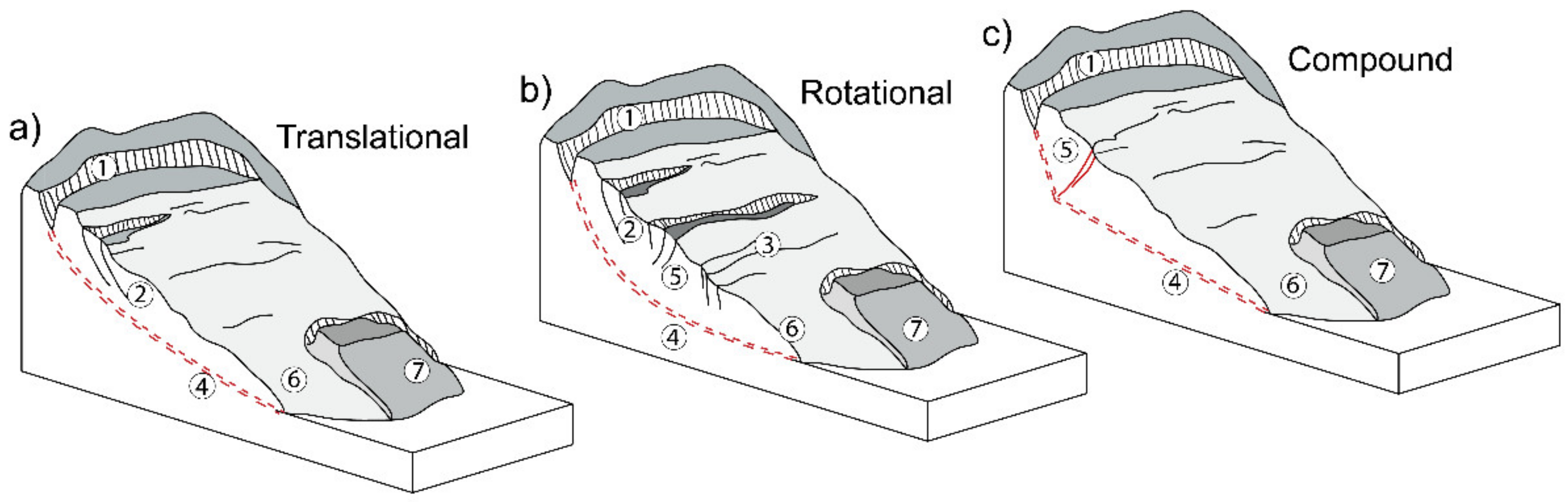
Slow rock-slope deformations are widespread in mountain ranges worldwide [14,15,16,17] and involve enormous rock volumes (up to billions of cubic meters) significantly affecting landscape [18]. Their onset and evolution depend on factors such as rock type and structural controls, glaciation and deglaciation, long-term seismicity and hydrological forcing [12,19,20,21,22,23]. They pose significant risks related to potential long-term interactions with man-made infrastructures [24,25] and to the progressive failure processes eventually evolving into massive collapse of slope sectors [23,26,27]. Slow RSDs often have ill-defined lateral boundaries and basal shear zones (200–300 m deep and more) and are characterized by low displacement rates (<50 mm/year [7,11,28]) and strongly segmented or heterogeneous strain fields. Their dominant mechanisms (translational, or compound, Figure 1) can become very complex when different nested sectors exist [29], testified by the spatial patterns and differential activity associated to their morpho-structural evidence [20] and by the development of nested secondary landslides (Figure 1). Translational slow RSDs (Figure 1a) are mainly characterized by downhill-facing scarps, while phenomena with rotational kinematics (Figure 1b) have curved headscarps, complex association scarps, and uphill-facing scarps (i.e., counterscarps) that accommodate rigid-body rotation in the middle–upper slope sectors. Finally, compound kinematics (Figure 1c) shows intermediate evidence of rotational and translational mechanisms.
The main characteristics of slow RSD (i.e., size, low rate, kinematic complexity) make them suitable to test the efficacy of a kinematics assessment approach based on 2D profiles. In addition, this approach is often the only feasible one, since these phenomena are so deep that they undergo boreholes and geophysical investigations only in special conditions, e.g., when interacting with extremely valuable assets as hydroelectric power facilities [20,30].
In the past, slow rock slope deformation study was limited by the low spatial coverage and resolution of monitoring techniques, either unable to detect very small displacement rates [31] or to capture displacement patterns over space and time. PSI techniques, including PS-InSAR™ [8] and SqueeSAR™ [32], proved their capability to measure small ground deformations with millimetric precision, making them suitable for regional-scale landslide mapping and inventory studies [7,11,33,34,35]. However, despite the improvements and refinements introduced by these methods, several limitations [34] still affect the application of DInSAR to landslide investigation.
A major limit of the technique is the inability of the satellite sensor to record the real 3D components of ground displacement, catching only the satellite line-of-sight LOS projection of any possible 3D ground deformation. Therefore, when the true deformation vector differs from the LOS, the sensitivity decreases and the interpretation of InSAR deformation measurements becomes challenging [10]. The application to the study of slow RSD is then further complicated because of low signal to noise ratio, presence of vegetation that can reduce the number of available PS and ambiguities related to the complexity and heterogeneity of landslide mechanisms [9]. The characterization of slow heterogeneous movements of large RSD has thus been commonly limited to recognize their degree of activity (mean velocity), and their potential to infer their kinematics is not obvious.
In this work, using PSI data derived from C-band Sentinel-1 A/B we evaluate the suitability of different descriptors and profile extraction approaches to infer landslide kinematics and outline spatial variations in movement rates in order to provide a best practice approach that can be applied also to other kind of phenomena.
2. Case Studies
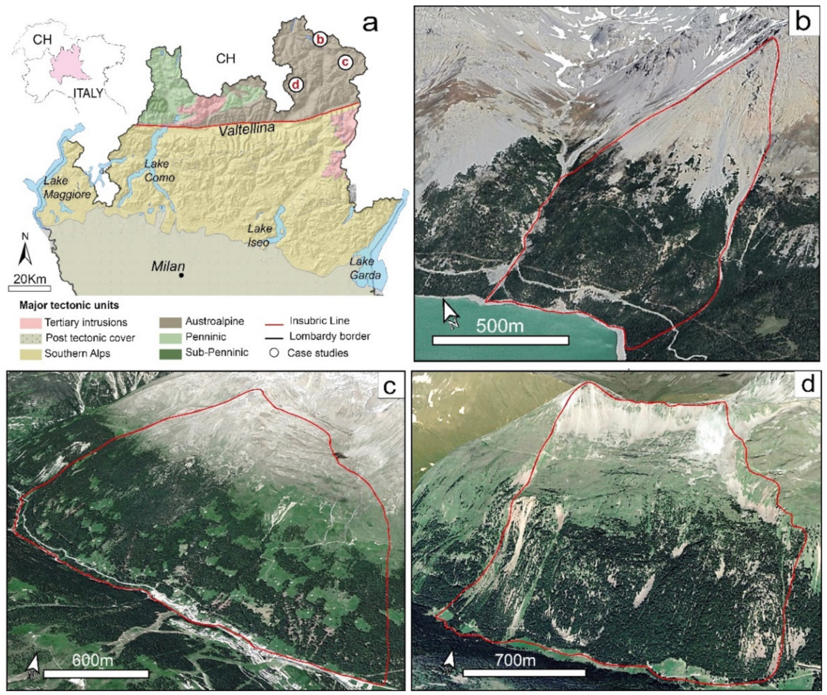
We selected as test sites three slow RSD (Figure 2a) representative of different deformation pattern, displacement rates and potential geohazard impact. These are Mt. Solena (Val Fraele Figure 2b), Corna Rossa (Valfurva, [29,36], Figure 2c) and Farinaccio (Val Grosina [11,13], Figure 2d), all actively deforming at different rates between 5 and 13 mm/year with local peaks reaching values of 20 mm/year. They are located in the north-eastern sector of Valtellina (Figure 2a, North Italy) in the Austroalpine domain. Mt Farinaccio and Corna Rossa slopes are made of polydeformed metamorphic rocks, mainly paragneiss, micaschists and phyllites belonging to the Grosina–Tonale and Campo nappes, respectively. Mt Solena is carved in Mesozoic limestone and dolomite of the Ortles Nappe [37,38].
All the three RSD affect high energy relief slopes (>1000 m) with a mean slope inclination of 30° affecting areas ranging between 1 and 10 km2. Their onset can be linked to the post-LGM destabilization of the valley flanks by means of progressive failure processes [23]. They are characterized by evident superficial morphostructures (e.g., Mt. Farinaccio), are part of ground based monitoring networks and affect critical scenarios (e.g., Mt. Solena impending over Cancano Lake and dam) and provide good examples of complex and segmented phenomena undergoing differential style of deformation (e.g., Corna Rossa) with nested sectors possibly evolving towards catastrophic collapse.
For each of them we performed a geomorphological mapping by means of detailed stereoscopic photo-interpretation of aerial imagery (Regione Lombardia TEM1 series, 1981–1983; nominal scale 1:20,000), digital orthophotos (2000; resolution 1 m, 2007, 2012, 2015; resolution 0.5 m), GoogleEarth™ imagery and Digital Elevation Models (Regione Lombardia, cell size: 5 m) in order to map major slope-scale features as well as local scale structures.
The main goal of this semi-detailed mapping [1] is to maximize the information at the slope scale thus providing a consistent dataset to be used as support for a kinematic and long-term activity analysis and give clues on the deformation and damage degree of each phenomenon. The integration between morphostructural information and PSI data is then necessary for a complete assessment of the style of activity of the landslides and provides a reading key to correctly interpret the ongoing displacement.
3. Workflow and Analyses
Starting from the state of the art [10,11,39] we suggest a methodological workflow that combines PSI data, morphostructural field evidence and simplified 2D finite element (FEM) models to retrieve a reliable description of the kinematics of the phenomena.
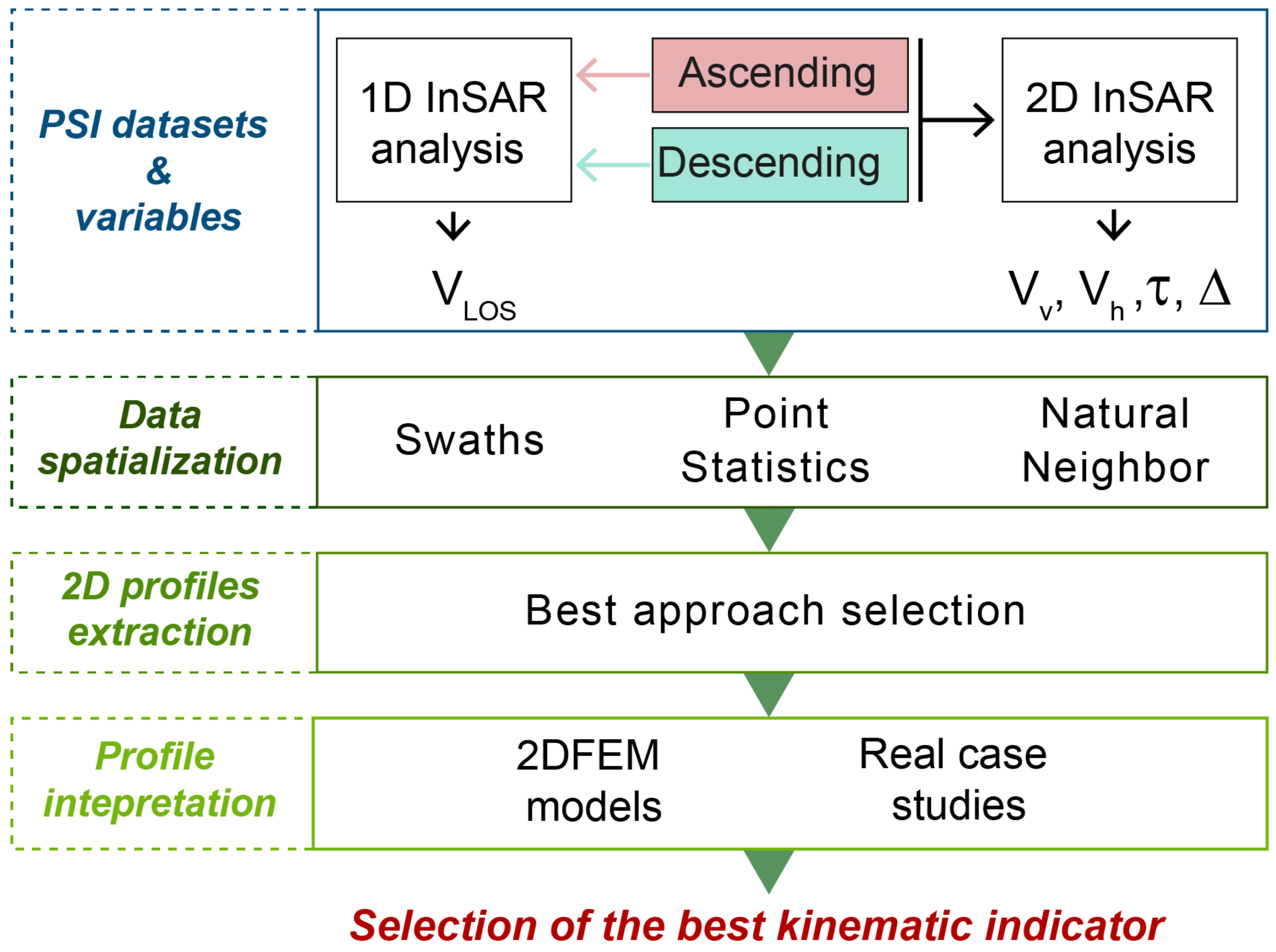
We perform the following analyses (Figure 3):
- 1-
- PSI data post-processing to extract quantities suitable to describe landslide kinematics;
- 2-
- spatial analysis of (point-like) PSI data to select profile traces representative of landside complexity (swath profiles) and distribute the information over landslide area (interpolation);
- 3-
- extraction of 2D profiles and assessment of the most suitable approach;
- 4-
- interpretation of 2D profiles using non-specific templates derived from simplified 2D FEM models and comparison to field evidence of selected case studies.
3.1. PSI Datasets Post-Processing and Kinematic Descriptors
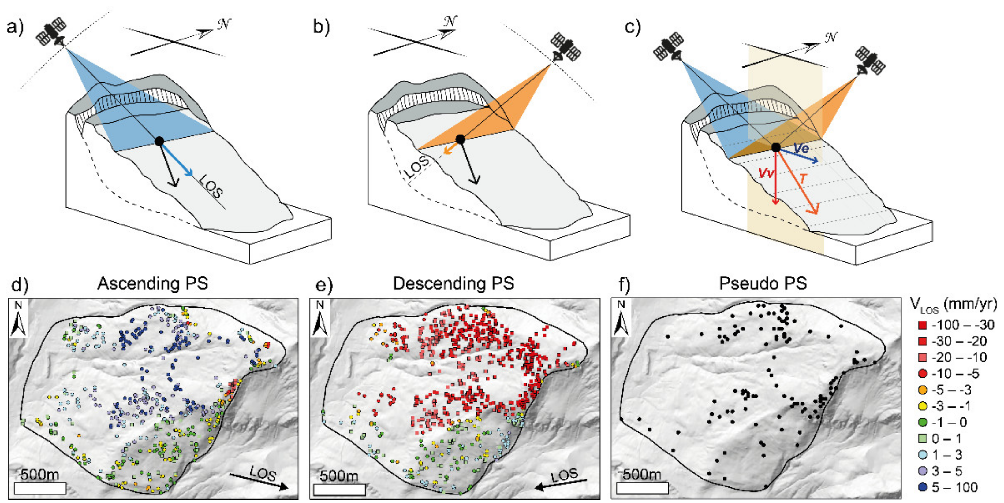
For our analysis, we used commercially available SqueeSAR™ datasets (TRE Altamira Table 1) derived from Sentinel1 A/B dataset acquired between 2015 and 2017 in both ascending and descending mode (Figure 4).
The simple examination of LOS velocity (VLOS) is the most straightforward way to investigate the style of activity of a landslide, but for a correct interpretation, it is necessary to take into account the LOS parameters and the slope topography (slope, aspect, etc.) to estimate how much of the true 3D displacement vector can be observed [11,40].
Some authors tried to overcome this issue by approximating the movement to a surface-parallel displacement, as in the case of ice flows analysis [41], projecting the LOS velocity along slope (Vslope [2,40,42]). This facilitates the interpretation of VLOS data and maximizes the data availability, but since it assumes a global translational sliding, it hampers any unconstrained interpretation of the landslide kinematics [11,43]. This is especially true for phenomena such as complex landslides, in which the internal displacement pattern can vary and differ from a simple slope-parallel movement.
The integration of InSAR displacement data from ascending and descending satellite orbits can help increasing the sensitivity for displacements close to the blind plane spanned by the two LOS vectors.
However, as the azimuth displacement components cannot be retrieved by the sensor, the ascending and descending radar LOS directions are simplified as both belonging to the East–West plane (Figure 4c).
We thus combined the two datasets through a 2DInSAR decomposition approach [10,44,45] and extracted the displacement vector components (Figure 4c,f).
First, since shallow movement associated with PSI point-like data can be induced by the instability of slope deposits (e.g., scree, glacial, or periglacial features) rather than by deep-seated deformations [11,43], we removed points inside superficial deposits based on available geomorphological maps [1] refined by original mapping on Google Earth™ imagery and recent orthophotos.
Moreover, as different acquisition geometries see different objects and each InSAR data stack has dissimilar sets of measurement points [46], we divided the area into regular square cells (size: 25 m) and for each cell assigned to the cell centroid (Pseudo PS) the average LOS velocity of PS and DS from the same acquisition geometry.
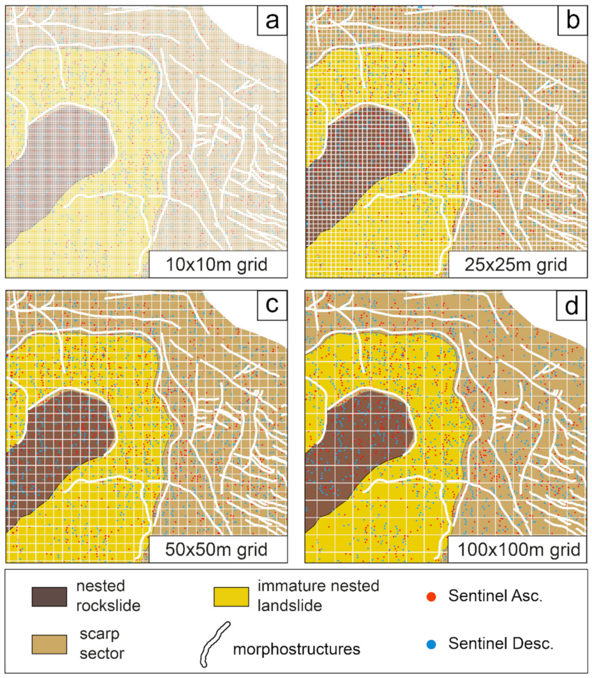
Grid size was selected after parametrically testing different cell dimensions (Figure 5).
Very small grid cell size 10 m (Figure 5a), below the spatial resolution of the sensor, in this case Sentinel-1, about 20 m, results in a reduced probability of finding Pseudo-PS (i.e., cell centroids combining information from both ascending and descending data). At the same time wide cells (50–100 m, Figure 5c,d) may extend over sectors characterized by different degree of activity and kinematics (i.e., over nested landslides boundaries) mixing up different signals and resulting in a smooth slope response. We thus selected an intermediate grid size of 25 m (Figure 5b) since it provides a fair discretization of the slope and it almost coincides with the mean distance computed between the points of the ascending and descending datasets (~24.58 m).
For each gridded point (pseudo-PS) we extracted the vertical (Vv) and horizontal (Ve) components and the 2D total displacement vectors (VT) [10]:
where Va and Vd are the ascending and descending LOS velocities (mm/year), and θa and θd are the incidence LOS angles for the considered satellite platform in the two acquisitions geometries.
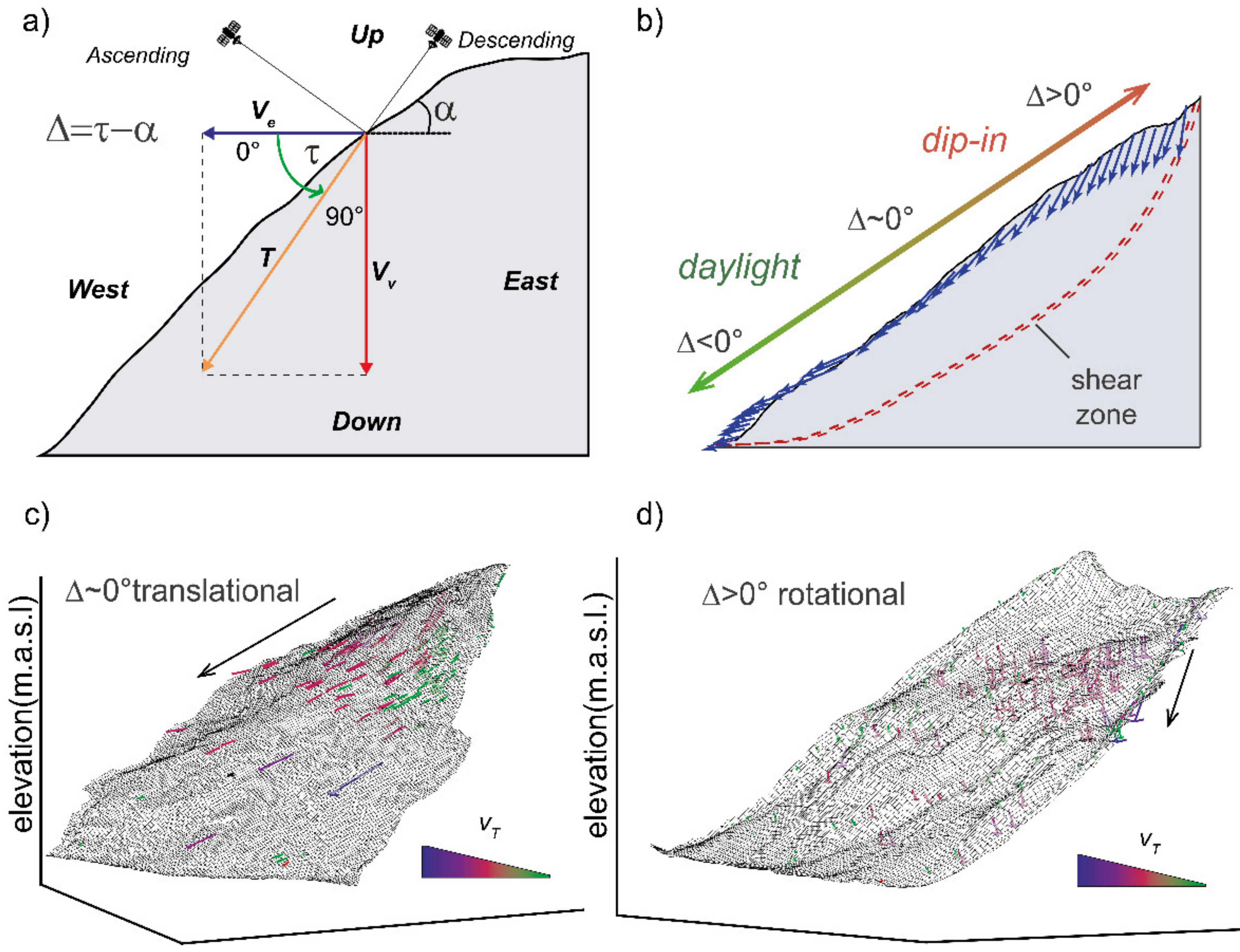
Depending on the failure mechanism, the superficial slope movement has different components along the landslide body and consequently Vv, Ve and τ change too (Figure 6a). Close to the main headscarp, the displacement vectors have a downward movement [11] and the total vector plunges at high angle into the slope (Figure 6b). In the middle and lower part, the horizontal component tends to become dominant and T vector usually becomes parallel to the slope or points upward in response of the toe uplifting (Figure 6b). Therefore, the displacement distributions may be used as a tool for interpreting the different geometry of the sliding surface for landslides of different typology and to identify active structures on the slope.
A first assessment of the local (i.e., cell-scale) slope kinematics can be inferred by observing the difference between τ and the local slope dip (α) in each square cell, namely Δ (Figure 6a,b):
3.2. Data Spatialization
To prepare the extraction of 2D kinematic profiles, we used three different spatial analysis methods to highlight the main issues possibly arising from each different approach.
As first approach, through an original Matlab™ tool we generated longitudinal swath profiles, corresponding to segments perpendicular to the down-slope direction in which the statistics of the displacement rate and pseudo-PS geometric information are calculated. Swath profiles are spatial analysis tools commonly used in geomorphometry [11,47,48], but also already applied to the extraction of landslide velocity values along 2D slope profile traces. Frattini et al. (2018) already used a similar method considering swaths extending up to the lateral boundary of the RSD. However, lateral variations due to changes in displacement vector direction with respect to the LOS, presence of secondary landslides or active structures, the geometry of the failure surface and the physical mechanical characteristics of the material [11] can significantly affect the summary interpretation of global kinematics along the considered slope profile.
To overcome this limitation and maximize the accuracy of the data, we implemented our Matlab™ tool to independently set the orientation and geometrical parameters of the swath (width, sampling step size) in a handy and interactive way. The profile trace can be arbitrarily drawn inside the landslide polygon, it is then subdivided in stripes perpendicular to the trace direction with variable length and width and inside each of them the mean value of PS data is calculated (Figure 6a,b).
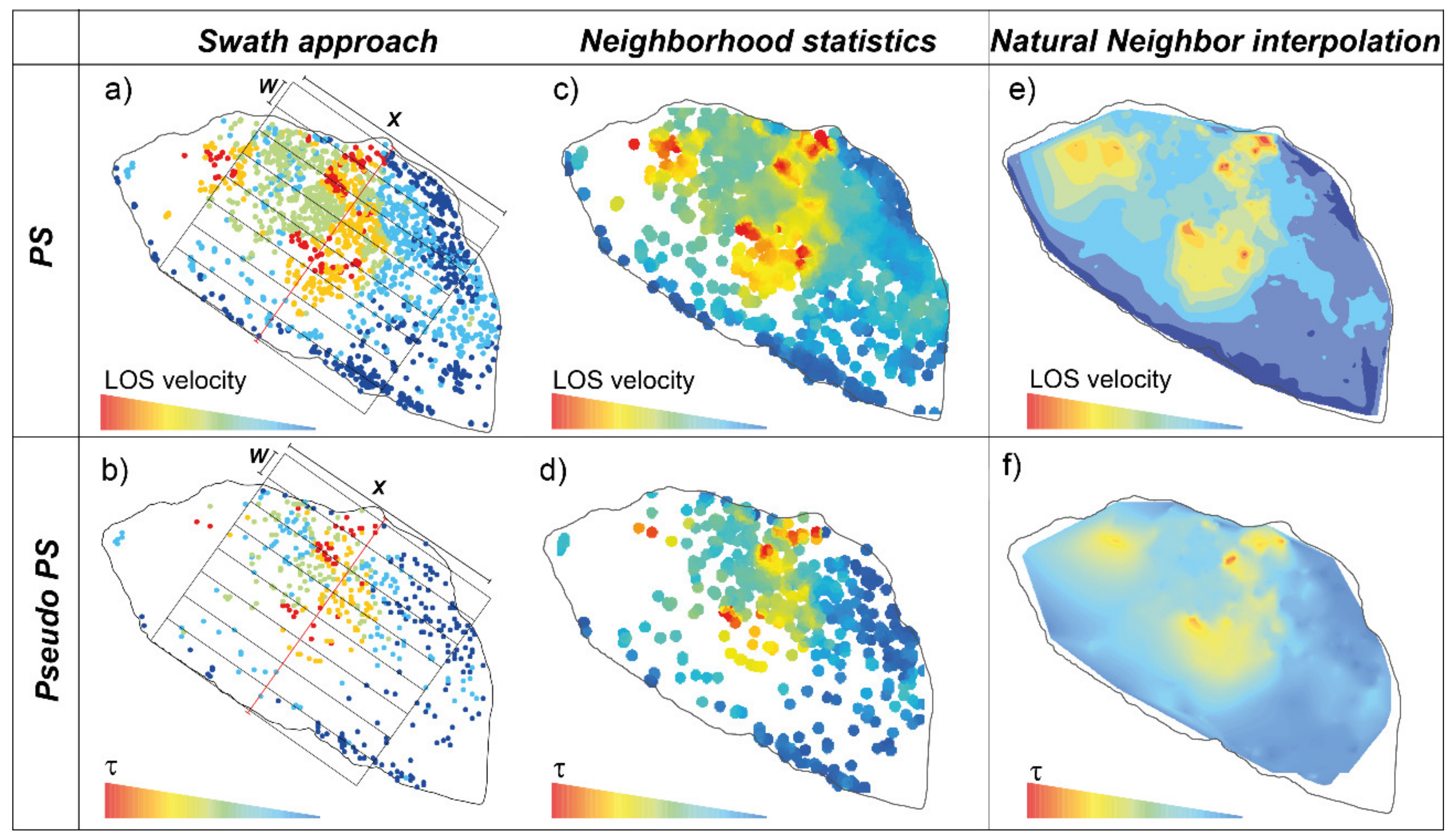
As second spatial analysis method, using the ArcGIS “Point Statistics” tool, we extracted for each PS and PseudoPS the average of the values falling within a specified neighborhood (5 cells). The final output is a raster where the value of each cell is function of the surrounding ones around that location (Figure 7c,d).
This is the most restrained spatial interpolator as it considers only the displacement values averaged on the PS itself and its closest neighbors. However, if points are too scattered, the raster map results discontinuous and the derived profile is strongly influenced by outliers or isolated values, thus compromising a correct interpretation.
As the third method, we tested a Natural-neighbor interpolation (Figure 6e,f). This latter finds the closest subset of input samples to a query point and applies weights to them based on proportionate areas to interpolate values [49]. This method preserves input data values and produces a continuous surface except at the sample points. We computed a 20 × 20 m grid and interpolated a surface bounded between PS and PseudoPS locations. No extrapolation was used to approximate values outside the convex hull.
3.3. Profiles Extraction
Because of internal segmentation, LOS velocity values are not usually constant through the slope and also the kinematic interpretation may vary from sector to sector.
In the case of complex landslides such as slow RSD, swath approach can thus be used as first tool to explore the spatial segmentation and to identify the most suitable profile trace to unravel the deep kinematics.
Variable dimensions (Figure 8a,b) highlight either the local movement of the sector close to the profile trace (narrow swath) or a mean displacement trend of a broader area (wide swath).
Considering PS LOS velocity information: keeping constant the longitudinal length of the swaths (100 m), a narrow swath size (50 m) gives a more precise response than a wider one (2000 m) as it emphasizes local changes in velocity with sharp peaks (Figure 8b), possibly corresponding to active morphostructures. A wide swath on the contrary averages a larger number of points that may belong to sectors with different kinematics and, as result, returns a smoother trend (Figure 8b). If the landslide has a complex behavior and internal segmentation, the use of wide swaths can be misleading for the analysis of the landslide activity and kinematics, whereas if the landslide is homogeneous and without strong strain partitioning, a wide swath [11] may be used to interpret the general deformation pattern. From this perspective, a comparison of profiles resulting from different swath dimension can be used as first tool to assess the activity heterogeneity and select the most representative profile traces, respectful of the spatial complexity. Swath width should be calibrated based on field and morphostructural observations.
Once a suitable profile trace has been selected, PSI data need to be interpolated over the landslide area in order to extract continuous profiles. Using swath profiles, a mean value is extracted inside each strip and its value can be very different from the one obtained through neighborhood statistics or natural neighbor interpolation in which weighted values are computed starting from the given interpolation points. Neighborhood statistics (point statistics) results strongly influenced by points distribution, emphasizing local response of isolated points and sharpening the values changes along slope in a more jagged profile than the one resulting from Natural Neighbor interpolation (Figure 8c,d).
In the following analyses we adopted natural neighbor interpolation to extract velocity and kinematic profiles and, to select the most reliable kinematic descriptor, we compared the effectiveness of possible geometric indicators (Vv, Ve, VLOS, τ, Δ) considering both synthetic 2D finite elements (2DFEM) models and real case studies with known kinematics.
3.4. Profiles Interpretation
3.4.1. DFEM Interpretation Templates
To get nonspecific reference templates representative of typical landslide kinematics, we performed simplified, 2D Finite-Element numerical simulations using the software RS2 (Rocscience Inc., Toronto, ON, Canada). Although based on a continuum small-strain formulation, the adopted code is able to account for deformation and failure mechanisms in both continuous and discontinuous rock masses [50,51].
For the simulations, we considered simplified slope geometries with constant slope gradient (30°) and characterized by imposed failure surfaces with different shape (translational, rotational, and compound) introduced as a Goodman joint element (pseudo-joints in continuum-based modeling) to constrain landslide kinematics. Slope height was set to 1200 m and failure surfaces traced at depth comprised between 200 and 400 m to simulate large RSD. These models do not cover the wide range of possible geometrical and mechanical conditions but are simply meant to extract the distribution of displacement components on simple failure surfaces.
The model domain was discretized into six noded triangular finite elements. Boundary conditions were assigned in terms of displacements (i.e., fixed bottom and side displacements), and a gravitational stress field was initializedWe attributed to the sliding mass values of strength and deformability parameters representative of common rock types (Table 2) as gneiss, schists, granitoids, plus idealized “very stiff” and “weak” rocks in order to extract a generic displacement signature for each kinematics. The non-deformed stable slope was constrained imposing an elastic behavior and high strength parameters.
We considered homogeneous materials characterized by an elasto-plastic behavior according to a Mohr–Coulomb failure criterion and we ran the simulations using the SSR (Shear Strength Reduction) technique, which allows to evaluate the Strength Reduction Factor associated with computed stress-displacement fields and failure mechanisms [52]. We then considered for each model the best SRF stage displaying the most evident kinematic deformation style and the critical stability conditions.
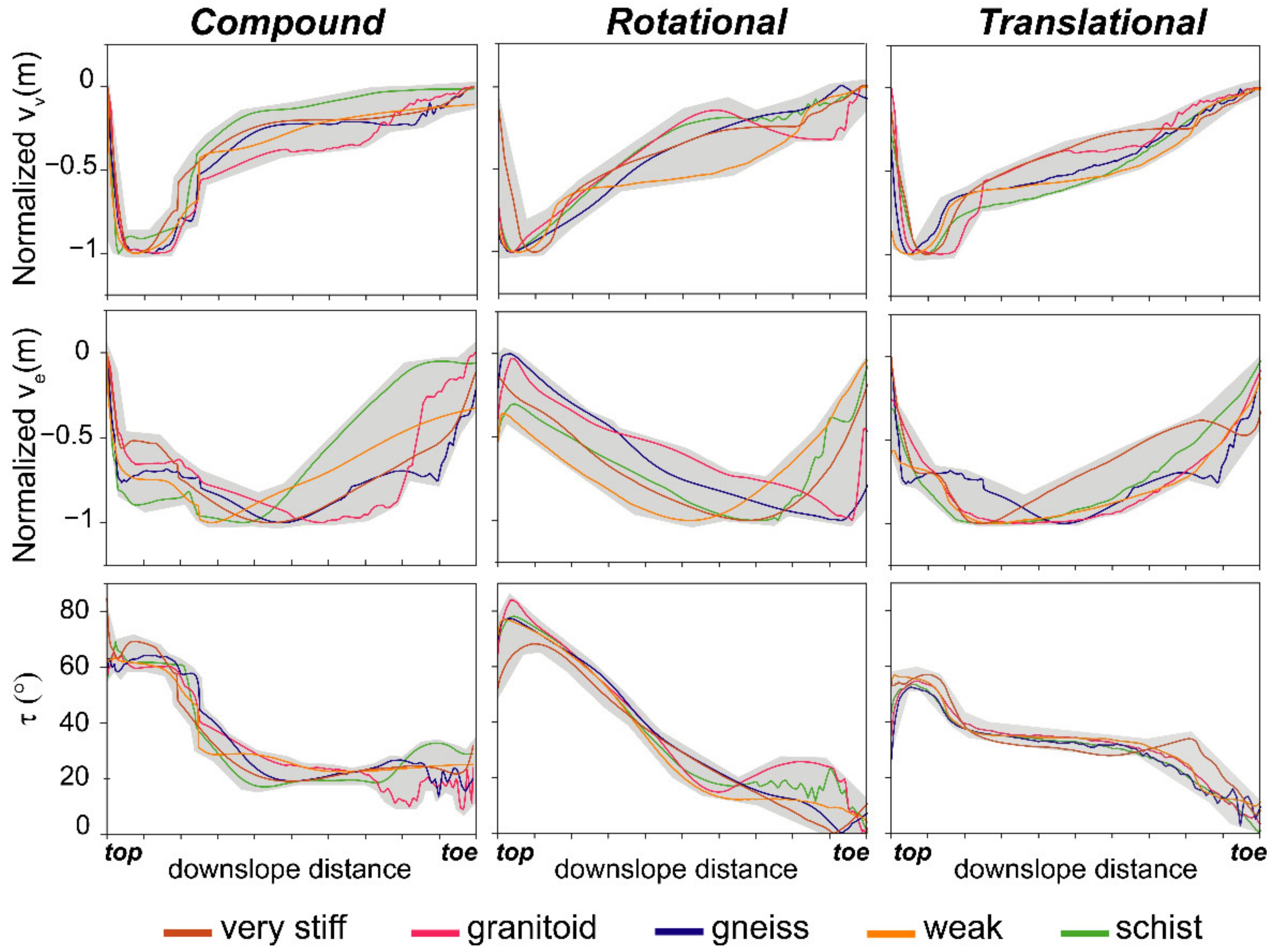
For each model, vertical (Vv), horizontal (Ve) and 2D total displacement inclination (τ) values were extracted along slope and plotted in normalized distance-displacement graphs (Figure 9).
A constant decrease in vertical values (Figure 9) from the top to the toe of the slope is typical of rotational kinematics as the sliding surface is steep in the upper slope sector and then becomes progressively parallel or gently dipping into the slope. A perfect rotational kinematics may also present daylight τ values at the toe, corresponding to bulging induced by rock mass push.
On the contrary, translational and compound mechanisms are characterized by almost constant vertical values (Figure 9) that tend to stabilize in a plateau that becomes more evident for rigid rocks. Localized higher vertical components correspond to the headscarp sector as clearly shown in the compound mechanism (Figure 9) where the most of the deformation is accommodated in an active wedge at the top of the slope connected through antithetic structures to a sliding sector (Figure 1c). It must be noticed that the vertical component can be strongly influenced by local conditions or by the rheological influence of the model as well as by differential internal deformation due to the mesh properties or geometric setting. Similarly, the horizontal component Ve (Figure 9) is less meaningful because it is strongly biased by the geometry of the model and does not provide clear signatures of different kinematic styles.
A flat pattern, corresponding to a constant dip angle, is typical of translational landslides (Figure 9) where the sliding movement is manly parallel to the slope, while for rotational kinematics it presents a highly decreasing angle going from the main headscarp (top) to the toe. Compound mechanism (Figure 9) is a combination of the previous two, as it shows highly plunging vectors in the headscarp sector, followed by translational movement along slope, mirrored by almost constant τ values. This suggests that, as τ, also Δ parameter can be considered a valid indicator of slope kinematics since it is directly linked to τ value and the local slope inclination. (Equation (5)) and gives a more accurate insight on the local deformation pattern.
3.4.2. Interpretation Using Geomorphological Mapping
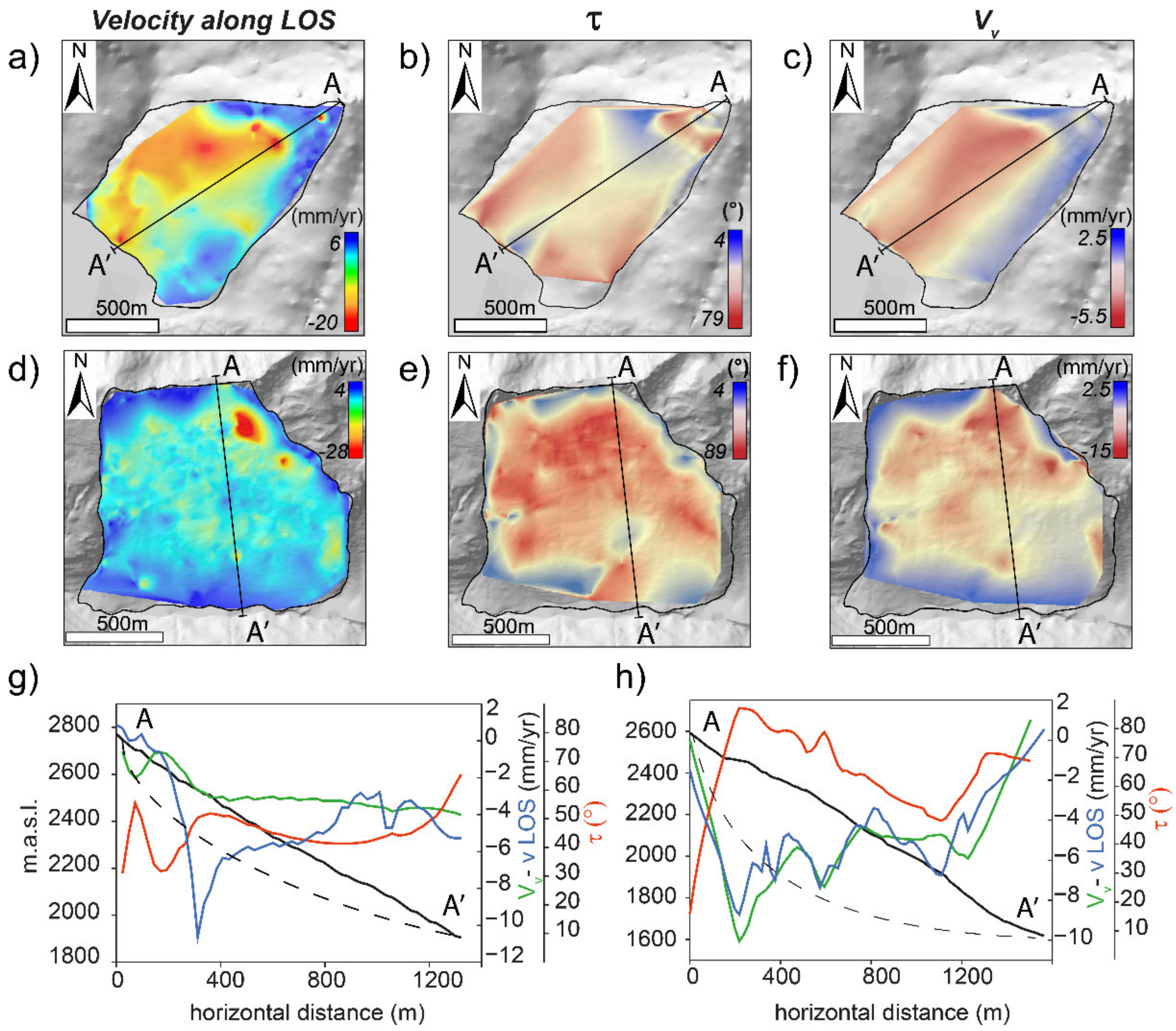
We compared the 2D kinematics profiles extracted from 1D VLOS distribution with geometrical information of Vv and τ resulting from the 2DInSAR analysis. We did not consider the horizontal displacement rate Ve since it represents the horizontal movement on a 2D E-W vertical plane and its values can be highly biased on slope with unfavorable orientation (Figure 10). On the contrary the vertical velocity represents the upward/downward displacement rate and gives more significant information on the landslide gravitational movement.
The profiles extracted for the Mt. Solena slope (Figure 10a–c) reflect a drop in Vv values (Figure 10g) close to the headscarp, that going downslope tend to stabilize around a steady value of about −3.5 mm/y, suggesting that the entire mass is uniformly moving and there are no active structures that induce important vertical movements. Similarly, τ profile (Figure 10g) confirms this observation with only few local fluctuations in the top slope sector and at the toe. Instead, LOS velocity profile (Figure 10g) sharply decreases in the upper slope portion to then rise towards less negative values towards the toe. The simple interpretation of 1D LOS profile may thus result misleading since the change in LOS velocity is not directly reflected by a change in kinematic style and a rise in VLOS may be improperly interpreted as signature of a rotational movement, while only corresponding to a faster sliding sector.
Mt. Farinaccio (Figure 10d–f), shows very similar Vv and LOS curves because the slope has an unfavorable orientation, almost N-S, with sliding direction towards S and E-W component almost null. As consequence, since in the 2DInSAR approach the N-S component is set to zero and the Ve is very small, LOS velocity and the vertical component tend to coincide. τ profile can be more easily interpreted since it shows dipping displacement vectors in the upper sector (Figure 10h) of the slope, corresponding to the main headscarp, which then decrease downslope as the movement becomes less steep, suggesting sliding on a surface that progressively becomes more parallel to the slope.
These considerations are also supported by the results of 2D FEM models that point out as τ (i.e., the inclination of the 2D displacement vector) is the most stable parameter to interpret the landslide kinematics since it describes geometric variations in the mechanics of the phenomenon more than bare velocity changes (Figure 11).
As consequence, the related Δ value, that corresponds to the difference between τ and the local slope angle (Equation (5)) can be exploited to investigate local surface variations (uplift, subsidence, etc.).
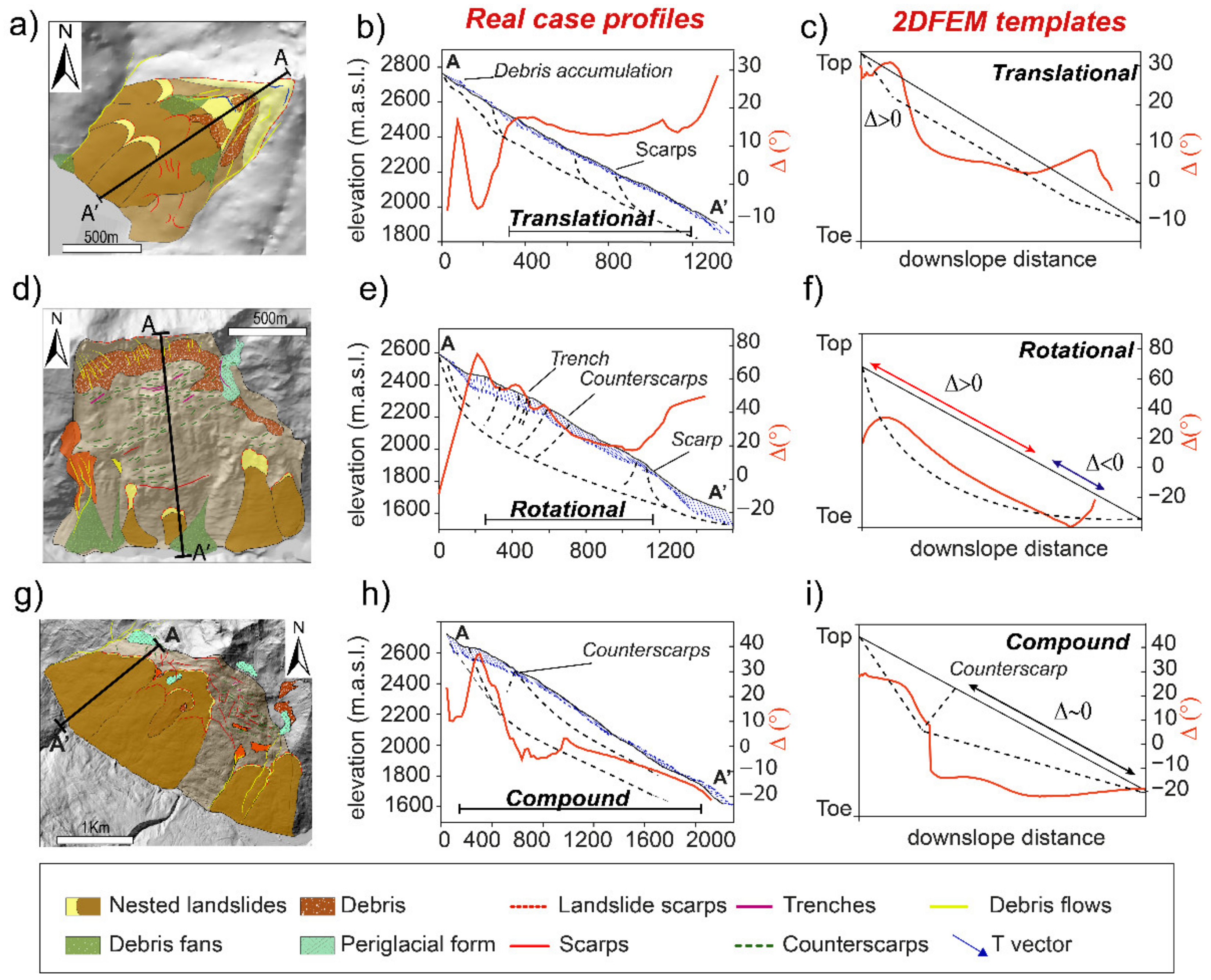
In Monte Solena (Figure 11a), Δ values have an almost constant value and the 2D displacement vector remains almost parallel to the slope (Figure 11b), as in the case of a modelled simple planar surface in which the type of movement is strongly limited (Figure 11c).
Changes in the profile trend correspond to mapped areas of debris accumulation and nested shallower phenomena.
A different scenario can be depicted for Mt. Farinaccio (Figure 11d). Δ shows highly dipping angles in the upper sector (Figure 11e) of the slope corresponding to the main headscarp and then decreases downslope, but always remaining steeply plunging into the slope. This trend is typical of rotational phenomena (Figure 11f) and local fluctuations are due to the presence of active morpho-structures highlighted in the mapping.
Corna Rossa (Figure 11g) is a more complex phenomenon [11,29,36] with a strong internal segmentation as anticipated in Figure 7 by swath profiles of increasing lateral length. This is due to a strong structural control that induce the onset of contiguous sectors actively deforming with different mechanisms expressed by distinctive morphostructural associations of scarps and counterscarps. The westernmost sector is characterized by an association of scarps in the upper sector and counterscarps and the relative Δ profile shows a double pattern: first it decreases in the headscarp sector and then it stabilizes on a slightly decreasing trend (Figure 11h) from 2000 m.a.s.l. to the valley floor. Comparing this pattern with the 2DFEM template, we can describe the kinematic as compound with a rotational uppermost wedge followed by a mainly sliding part (Figure 11i).
4. Discussion
A robust kinematic characterization is fundamental to understand landslide mechanisms, interpret their controls, and predict their potential evolution to plan appropriate risk mitigation strategies. Despite having the same displacement rate, different landslides may in fact behave in different ways both in an evolutive and risk perspective according to their deformation style, involved rock mass volumes, interaction with at risk elements and collapse potential [53,54]. To this aim, PSI data have been widely applied to extract an activity and kinematic analysis [9,10,11], but an in-depth investigation of the most suitable geometric descriptor has never been conducted.
In this study, we exploited the use of commercial [8,33] PSI products to investigate their effectiveness in unravelling the kinematics of slow RSD that are among the most complex landslides and can be thus considered the most complete test cases on which validate the analyses [55].
We propose a practical workflow to: (a) identify the most suitable, unbiased descriptors of landslide kinematics; (b) maximize the potential of sparse PSI data to obtain continuous 2D profiles; (c) obtain constraints on the kinematic interpretation of 2D profiles.
First, to retrieve the real kinematic behavior it is necessary to refine PS datasets to remove those points lying in the superficial debris cover or periglacial forms that can have differential movements and introduce false signals in the analysis. Then, it must be taken into account that the near polar orbit of the satellite causes the impossibility to obtain readings in the NS direction, which in some case, such as Mt. Farinaccio RSD, is the principal direction of sliding, essentially impeding the analysis of horizontal velocity from PSInSAR™ measurements. However, exploiting these data through a 2DInSAR approach, thus combining the ascending and descending datasets in the same time span and with a high spatial density, it is possible to increase the sensitivity of the measure and extract geometrical information associated with the 2D displacement vector.
Using appropriate spatial analysis approaches, point-like information can be then visualized and investigated through along slope profiles arbitrarily traced. In particular, using swaths with variable dimensions it is possible to assess a first degree of the landslide heterogeneity and select the most representative profile trace. Afterward, the use of a Natura Neighbor interpolation allows to obtain a spatial coverage of the information over the landslide area, yet preserving the original value of the PS or PseudoPS point, and to extract continuous profiles.
Their interpretation was then supported by nonspecific templates from 2DFEM models and real case investigations, that proved the effectiveness of profiles in describing the landslide kinematics. The integration of these two approaches first gives an insight on the most suitable kinematic descriptors, that are found in the inclination of the 2D displacement vector (τ) and the associated Δ value, corrected for the local slope angle. Furthermore, it allows to unravel both the general kinematic signature of the analyzed landslide, controlled by the rock rheology and the geometry of the sliding surface, and the presence of local spatial heterogeneities, induced by nested shallower phenomena, active morphostructures and highly damaged zones recognized from the mapping.
This approach can be thus applied to analyze even complex landslides with heterogeneous strain distribution. A peculiar example is provided by Corna Rossa (Figure 11g and Figure 12) characterized by a strong structural control, mirrored by distinctive morphostructural associations and slope segmentation [29,36]. The NW slope sector is affected by several orders of scarps, while the SE area is dissected by steep scarps and counterscarps arranged in a graben system [29,36].
The transition between these two sectors is marked by the abrupt closing of the NW sector main scarp in correspondence of the graben system and by persistent scarps which are oriented towards NNW-SSE.
Different features are ascribable to different deformation mechanisms and suggest a transition from a mainly sliding sector to a “spreading” one, characterized by dominant extension accommodated by symmetric and asymmetric graben structures [29,36].
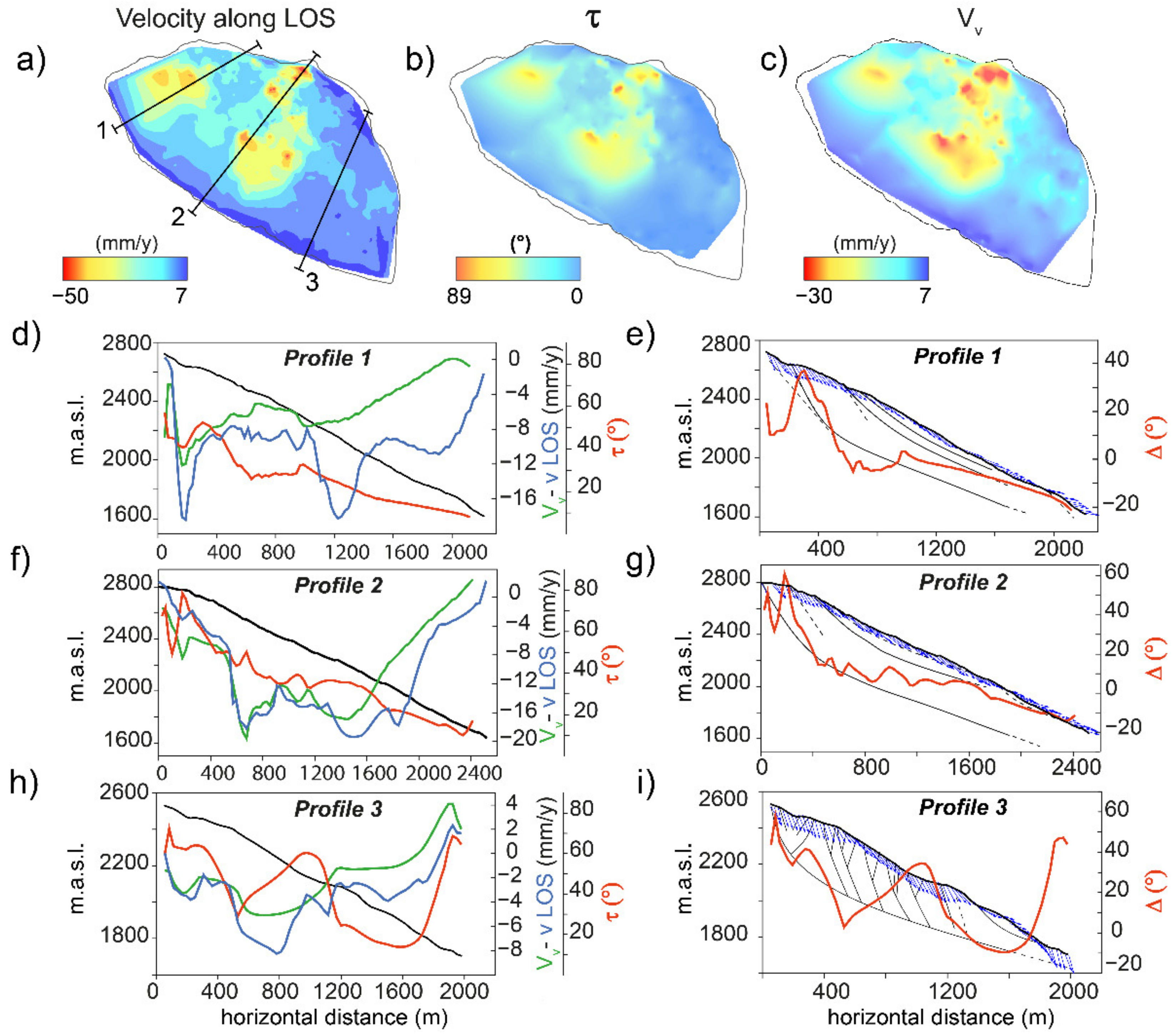
This change in kinematic behavior, inferred from morpho-structural observations, is confirmed by τ and Δ profiles (Figure 12b,c). From NW to SE we can recognize a transition from a compound sliding (Figure 12d,e) with 2D displacement vectors oriented almost parallel to the slope (Figure 12e), to a dominant rotation-rototranslation (Figure 12f,g) and a more complex kinematic (Figure 12h,i) strongly influenced by the presence of deep scarps and counterscarps arranged in a graben system (Figure 12i).
τ and Δ profiles well reflect the deep deformation style because, even if the LOS velocity is underestimated or biased, the combination of two different acquisition geometries provides a depictive inclination angle of the 2D displacement on the E-W vertical plane. The more the slope is favorably oriented, and the sliding occurs in the E-W direction, the more τ corresponds to the true inclination angle and the kinematic interpretation becomes straightforward. As we depart from the LOS plane, we can generally expect to underestimate the 2D displacement vector inclination, resulting in a less effective detection of rotational movements and the integration with morphostructural evidence becomes fundamental for a correct interpretation of the deformation style.
In general, when the cross-section is not aligned E-W and when the movement vectors are oblique, the E-W movement vectors are reprojected along the cross-section as if the maximum movement occurs along the steepest slope direction. However, if a landslide experiences oblique movements, when the vectors are reprojected along the cross-section, their horizontal component will be much more underestimated with respect to the vertical one [56]. As consequence, the interpretation of 1D VLOS profiles is not always straightforward in the assessment of kinematics because they can present peaks and fluctuations linked to heterogeneous velocity and isolated high values more than true kinematic transitions. Negative or positive peaks can outline active structures or nested phenomena that, despite having different displacement rates, keep the same deformation style (e.g., fast or slow sliding sectors).
By extracting 2D profiles of different descriptors, in principle suitable for kinematic characterization, we showed that a velocity analysis based on 1D LOS velocity values (VLOS) is not suitable to unambiguously represent landslide kinematics, especially when with complex phenomena such as slow RSD. These are characterized by sectors with different activity, kinematics and heterogeneous strain fields, and the single use of VLOS values results less robust and partially ineffective in describing the response of each slope sector. At the same time, the kinematics also influences the percentage of movement that can be sensed along the LOS thus resulting in different representative LOS velocities that only capture part of the total displacement vector thus returning a partial velocity information. Instead, the combination of data from different geometries captured with different LOS increases the sensitivity to displacement and reduces the complexity related to interpretation of InSAR data [10].
A 2DInSAR analysis should therefore be preferred, using the derived τ angle in combination with digital elevation model to identify areas undergoing displacement into (Δ > 0) or out of slope (Δ < 0) [57]. A limiting side of this approach is that the resulting 2D displacement is “forced” to lay in the EW plane, affecting the estimated horizontal (EW) and vertical components of the 3D displacement vector. To correctly quantify the components of the 3D vector, additional information must be provided along other LOS directions such as additional satellite tracks, ad hoc UAVSAR acquisitions, GPS data, offset pixel tracking. Summing up, our analysis proved that even at local scale, commercial PSInSAR™ data combined with field observation and validated by means of 2DFEM models, can play an important role in interpreting the kinematics of landslides, but to be able to give exact estimates on the true inclination and magnitude of the 3D displacement vector, a combination of in situ instrumentations, detailed mapping of landforms and geological structures is needed [10].
5. Conclusions
Recognizing the kinematics of a landslide is a major task to characterize its evolution and predict its potential impact on infrastructures and elements at risk. However, the definition of a proper kinematic style becomes particularly difficult for complex slow RSD, and the study of this is hampered by the limited amount of available data and the low displacement rate (mm to cm per year).
In this study, we exploited commercial PSI data to identify the most suitable kinematic descriptor of slow RSD and we provided a general overview of the limitations and advantages of this technique in the study of this complex class of landslides.
We highlight how a single 1D LOS analysis is not sufficient to describe complex landslide kinematics and a multi geometry 2DInSAR approach should be preferred as it provides a powerful tool for visualizing local vector geometry. We compare different geometrical descriptors using data spatialization approaches and profile extraction techniques respectful of the landslide heterogeneity and we integrate their interpretation with morphostructural mapping and 2DFEM results, retrieving a final consistent kinematic characterization.
Author Contributions
Conceptualization, methodology, investigation and validation: C.C. and F.A.; formal analysis and writing—original draft preparation, C.C.; writing—review and editing, F.A.; supervision, funding acquisition, F.A. All authors have read and agreed to the published version of the manuscript.
Funding
The research was supported by Fondazione Cariplo grant 2016-0757 “Slow2Fast” to F.A. and by the MIUR—“Dipartimenti di Eccellenza 2018–2022, Department of Earth and Environmental Sciences, University of Milano-Bicocca”.
Institutional Review Board Statement
Not applicable.
Informed Consent Statement
Not applicable.
Acknowledgments
We thank Elena Valbuzzi for her support to geomorphological mapping of case studies. We thank the editor and two anonymous reviewers for their constructive comments.
Conflicts of Interest
The authors declare no conflict of interest.
References
- Crippa, C.; Valbuzzi, E.; Frattini, P.; Crosta, G.B.; Spreafico, M.C.; Agliardi, F. Semi-automated regional classification of the style of activity of slow rock-slope deformations using PS InSAR and SqueeSAR velocity data. Landslides 2021. [Google Scholar] [CrossRef]
- Aslan, G.; Foumelis, M.; Raucoules, D.; De Michele, M.; Bernardie, S.; Cakir, Z. Landslide mapping and monitoring using persistent scatterer interferometry (PSI) technique in the French alps. Remote Sens. 2020, 12, 1305. [Google Scholar] [CrossRef] [Green Version]
- Gullà, G.; Peduto, D.; Borrelli, L.; Antronico, L.; Fornaro, G. Geometric and kinematic characterization of landslides affecting urban areas: The Lungro case study (Calabria, Southern Italy). Landslides 2017, 14, 171–188. [Google Scholar] [CrossRef]
- Brückl, E.; Brunner, F.K.; Kraus, K. Kinematics of a deep-seated landslide derived from photogrammetric, GPS and geophysical data. Eng. Geol. 2006, 88, 149–159. [Google Scholar] [CrossRef]
- Travelletti, J.; Malet, J.-P. Characterization of the 3D geometry of flow-like landslides: A methodology based on the integration of heterogeneous multi-source data. Eng. Geol. 2012, 128, 30–48. [Google Scholar] [CrossRef]
- Wasowski, J.; Pisano, L. Long-term InSAR, borehole inclinometer, and rainfall records provide insight into the mechanism and activity patterns of an extremely slow urbanized landslide. Landslides 2020, 17, 445–457. [Google Scholar] [CrossRef]
- Wasowski, J.; Bovenga, F. Investigating landslides and unstable slopes with satellite Multi Temporal Interferometry: Current issues and future perspectives. Eng. Geol. 2014, 174, 103–138. [Google Scholar] [CrossRef]
- Ferretti, A.; Prati, C.; Rocca, F. Permanent scatterers in SAR interferometry. IEEE Trans. Geosci. Remote Sens. 2001, 39, 8–20. [Google Scholar] [CrossRef]
- Schlögel, R.; Doubre, C.; Malet, J.P.; Masson, F. Landslide deformation monitoring with ALOS/PALSAR imagery: A D-InSAR geomorphological interpretation method. Geomorphology 2015, 231, 314–330. [Google Scholar] [CrossRef]
- Eriksen, H.Ø.; Lauknes, T.R.; Larsen, Y.; Corner, G.D.; Bergh, S.G.; Dehls, J.; Kierulf, H.P. Visualizing and interpreting surface displacement patterns on unstable slopes using multi-geometry satellite SAR interferometry (2D InSAR). Remote Sens. Environ. 2017, 191, 297–312. [Google Scholar] [CrossRef] [Green Version]
- Frattini, P.; Crosta, G.B.; Rossini, M.; Allievi, J. Activity and kinematic behaviour of deep-seated landslides from PS-InSAR displacement rate measurements. Landslides 2018, 15, 1053–1070. [Google Scholar] [CrossRef]
- Agliardi, F.; Riva, F.; Barbarano, M.; Zanchetta, S.; Scotti, R.; Zanchi, A. Effects of tectonic structures and long-term seismicity on paraglacial giant slope deformations: Piz Dora (Switzerland). Eng. Geol. 2019, 263, 105353. [Google Scholar] [CrossRef]
- Agliardi, F.; Crosta, G.B.; Frattini, P. Slow rock-slope deformation. In Landslides: Types, Mechanisms and Modeling; Cambridge University Press: Cambridge, UK, 2012; p. 207. [Google Scholar]
- Crosta, G.B.; Frattini, P.; Agliardi, F. Deep seated gravitational slope deformations in the European Alps. Tectonophysics 2013, 605, 13–33. [Google Scholar] [CrossRef]
- Chigira, M. September 2005 rain-induced catastrophic rockslides on slopes affected by deep-seated gravitational deformations, Kyushu, southern Japan. Eng. Geol. 2009, 108, 1–15. [Google Scholar] [CrossRef]
- Audemard, F.A.; Beck, C.; Carrillo, E. Deep-seated gravitational slope deformations along the active Boconó Fault in the central portion of the Mérida Andes, western Venezuela. Geomorphology 2010, 124, 164–177. [Google Scholar] [CrossRef]
- Lin, C.W.; Tseng, C.M.; Tseng, Y.H.; Fei, L.Y.; Hsieh, Y.C.; Tarolli, P. Recognition of large scale deep-seated landslides in forest areas of Taiwan using high resolution topography. J. Asian Earth Sci. 2013, 62, 389–400. [Google Scholar] [CrossRef]
- Agliardi, F.; Crosta, G.B.; Frattini, P.; Malusà, M.G. Giant non-catastrophic landslides and the long-term exhumation of the European Alps. Earth Planet. Sci. Lett. 2013, 365, 263–274. [Google Scholar] [CrossRef]
- Bovis, M.J.; Evans, S.G. Extensive deformations of rock slopes in southern Coast Mountains, southwest British Columbia, Canada. Eng. Geol. 1996, 44, 163–182. [Google Scholar] [CrossRef]
- Agliardi, F.; Crosta, G.B.; Zanchi, A. Structural constraints on deep-seated slope deformation kinematics. Eng. Geol. 2001, 59, 83–102. [Google Scholar] [CrossRef]
- Crosta, G.B.; di Prisco, C.; Frattini, P.; Frigerio, G.; Castellanza, R.; Agliardi, F. Chasing a complete understanding of the triggering mechanisms of a large rapidly evolving rockslide. Landslides 2013, 11, 747–764. [Google Scholar] [CrossRef]
- Grämiger, L.M.; Moore, J.R.; Gischig, V.S.; Ivy-Ochs, S.; Loew, S. Beyond debuttressing: Mechanics of paraglacial rock slope damage during repeat glacial cycles. J. Geophys. Res. Earth Surf. 2017, 122, 1004–1036. [Google Scholar] [CrossRef]
- Riva, F.; Agliardi, F.; Amitrano, D.; Crosta, G.B. Damage-Based Time-Dependent Modeling of Paraglacial to Postglacial Progressive Failure of Large Rock Slopes. J. Geophys. Res. Earth Surf. 2018, 123, 124–141. [Google Scholar] [CrossRef] [Green Version]
- Ambrosi, C.; Crosta, G.B. Large sackung along major tectonic features in the Central Italian Alps. Eng. Geol. 2006, 83, 183–200. [Google Scholar] [CrossRef]
- Frattini, P.; Crosta, G.B.; Allievi, J. Damage to buildings in large slope rock instabilities monitored with the PSinSAR™ technique. Remote Sens. 2013, 5, 4753–4773. [Google Scholar] [CrossRef] [Green Version]
- Crosta, G.B.; Imposimato, S.; Roddeman, D.G. Numerical modelling of large landslides stability and runout. Nat. Hazards Earth Syst. Sci. 2003, 3, 523–538. [Google Scholar] [CrossRef]
- Eberhardt, E.; Stead, D.; Coggan, J.S. Numerical analysis of initiation and progressive failure in natural rock slopes-the 1991 Randa rockslide. Int. J. Rock Mech. Min. Sci. 2004, 41, 69–87. [Google Scholar] [CrossRef]
- Rott, H.; Scheuchl, B.; Siegel, A.; Grasemann, B. Monitoring very slow slope movements by means of SAR interferometry: A case study from a mass waste above a reservoir in the Otztal Alps, Austria. Geophys. Res. Lett. 1999, 26, 1629–1632. [Google Scholar] [CrossRef]
- Agliardi, F.; Crippa, C.; Spreafico, M.C.; Manconi, A.; Bourlès, D.; Braucher, R.; Cola, G.; Zanchetta, S. Strain partitioning and heterogeneous evolution in a giant slope deformation revealed by InSAR, dating and modelling. In Proceedings of the Geophysical Research Abstracts, Vienna, Austria, 7–12 April 2019; Volume 21. [Google Scholar]
- Jongmans, D.; Garambois, S. Geophysical investigation of landslides: A review. Bull. Soc. Géol. Fr. 2007, 178, 101–112. [Google Scholar] [CrossRef] [Green Version]
- Bovis, M.J. Rock-slope deformation at Affliction Creek, southern Coast Mountains, British Columbia. Can. J. Earth Sci. 1990, 27, 243–254. [Google Scholar] [CrossRef]
- Ferretti, A.; Fumagalli, A.; Novali, F.; Prati, C.; Rocca, F.; Rucci, A. A new algorithm for processing interferometric data-stacks: SqueeSAR. In IEEE Transactions on Geoscience and Remote Sensing; IEEE: Piscataway, NJ, USA, 2011. [Google Scholar]
- Colesanti, C.; Ferretti, A.; Prati, C.; Rocca, F. Monitoring landslides and tectonic motions with the Permanent Scatterers Technique. Eng. Geol. 2003, 68, 3–14. [Google Scholar] [CrossRef]
- Colesanti, C.; Wasowski, J. Investigating landslides with space-borne Synthetic Aperture Radar (SAR) interferometry. Eng. Geol. 2006, 88, 173–199. [Google Scholar] [CrossRef]
- Rosi, A.; Agostini, A.; Tofani, V.; Casagli, N. A Procedure to map subsidence at the regional scale using the persistent scatterer interferometry (PSI) technique. Remote Sens. 2014, 6, 10510–10522. [Google Scholar] [CrossRef]
- Agliardi, F.; Spreafico, M.C.; Zanchetta, S.; Castellanza, R.; Asnaghi, R.; Paternoster, J.; Crippa, C.; Crosta, G. Gravitational transfer zones influence DSGSD mechanisms and activity. In Proceedings of the EGU General Assembly Conference Abstracts, Vienna, Austria, 4–13 April 2018; Volume 20, p. 13819. [Google Scholar]
- Schmid, S.M.; Fügenschuh, B.; Kissling, E.; Schuster, R. Tectonic map and overall architecture of the Alpine orogen. Eclogae Geol. Helv. 2004, 97, 93–117. [Google Scholar] [CrossRef]
- Ferrari, F.; Giani, G.P.; Apuani, T. Towards the comprehension of rockfall motion, with the aid of in situ tests. In Proceedings of the Vajont Thoughts and Analyses after 50 Years Since the Catastrophic Landslide, Padua, Italy, 8–10 October 2013; Sapienza Università Editrice: Roma, Italy; pp. 163–171. [Google Scholar]
- Henderson, I.H.C.; Lauknes, T.R.; Osmundsen, P.T.; Dehls, J.; Larsen, Y.; Redfield, T.F. A structural, geomorphological and InSAR study of an active rock slope failure development. Geol. Soc. London, Spec. Publ. 2011, 351, 185–199. [Google Scholar] [CrossRef]
- Notti, D.; Herrera, G.; Bianchini, S.; Meisina, C.; García-Davalillo, J.C.; Zucca, F. A methodology for improving landslide PSI data analysis. Int. J. Remote Sens. 2014, 35, 2186–2214. [Google Scholar] [CrossRef]
- Joughin, L.R.; Kwok, R.; Fahnestock, M.A. Interferometric estimation of three-dimensional ice-flow using ascending and descending passes. IEEE Trans. Geosci. Remote Sens. 1998, 36, 25–37. [Google Scholar] [CrossRef] [Green Version]
- Notti, D.; Meisina, C.; Zucca, F.; Colombo, A. Models To Predict Persistent Scatterers Data Distribution and Their Capacity To Register Movement Along the Slope. In Proceedings of the Fringe 2011, Frascati, Italy, 19–23 September 2011; pp. 19–23. [Google Scholar]
- Meisina, C.; Zucca, F.; Notti, D.; Colombo, A.; Cucchi, A.; Savio, G.; Giannico, C.; Bianchi, M. Geological interpretation of PSInSAR Data at regional scale. Sensors 2008, 8, 7469–7492. [Google Scholar] [CrossRef] [PubMed] [Green Version]
- Manzo, M.; Ricciardi, G.P.P.; Casu, F.; Ventura, G.; Zeni, G.; Borgström, S.; Berardino, P.; Del Gaudio, C.; Lanari, R. Surface deformation analysis in the Ischia Island (Italy) based on spaceborne radar interferometry. J. Volcanol. Geotherm. Res. 2006, 151, 399–416. [Google Scholar] [CrossRef]
- Dalla Via, G.; Crosetto, M.; Crippa, B. Resolving vertical and east-west horizontal motion from differential interferometric synthetic aperture radar: The L’Aquila earthquake. J. Geophys. Res. Solid Earth 2012, 117. [Google Scholar] [CrossRef] [Green Version]
- Ferretti, A. Satellite InSAR Data: Reservoir Monitoring from Space; EAGE Publications: Houten, The Netherlands, 2014; ISBN 978-90-73834-71-2. [Google Scholar]
- Baulig, H. Sur une méthode altimétrique d’analyse morphologique appliquée à la Bretagne péninsulaire. Bull. Assoc. Geogr. Fr. 1926, 3, 7–9. [Google Scholar] [CrossRef]
- Grohmann, C.H. Morphometric analysis in geographic information systems: Applications of free software GRASS and R. Comput. Geosci. 2004, 30, 1055–1067. [Google Scholar] [CrossRef] [Green Version]
- Sibson, R. A Brief Description of Natural Neighbor Interpolation chapter 2. In Interpolating Multivariate Data; John Wiley & Sons: New York, NY, USA, 1981; pp. 21–36. [Google Scholar]
- Hammah, R.E.; Yacoub, T.; Corkum, B.; Curran, J.H. The practical modelling of discontinuous rock masses with finite element analysis. In Proceedings of the The 42nd US Rock Mechanics Symposium (USRMS), San Francisc, CA, USA, 29 June–2 July 2008. [Google Scholar]
- Riahi, A.; Hammah, E.R.; Curran, J.H. Limits of applicability of the finite element explicit joint model in the analysis of jointed rock problems. In Proceedings of the 44th US Rock Mechanics Symposium and 5th US-Canada Rock Mechanics Symposium, Salt Lake City, UT, USA, 27–30 June 2010. [Google Scholar]
- Dawson, E.M.; Roth, W.H.; Drescher, A. Slope stability analysis by strength reduction. Geotechnique 1999, 49, 835–840. [Google Scholar] [CrossRef]
- Agliardi, F.; Scuderi, M.M.; Fusi, N.; Collettini, C. Slow-to-fast transition of giant creeping rockslides modulated by undrained loading in basal shear zones. Nat. Commun. 2020, 11, 1–11. [Google Scholar] [CrossRef] [PubMed]
- Peduto, D.; Ferlisi, S.; Nicodemo, G.; Reale, D.; Pisciotta, G.; Gullà, G. Empirical fragility and vulnerability curves for buildings exposed to slow-moving landslides at medium and large scales. Landslides 2017, 14, 1993–2007. [Google Scholar] [CrossRef]
- Uzielli, M.; Catani, F.; Tofani, V.; Casagli, N. Risk analysis for the Ancona landslide—I: Characterization of landslide kinematics. Landslides 2015, 12, 69–82. [Google Scholar] [CrossRef] [Green Version]
- Intrieri, E.; Frodella, W.; Raspini, F.; Bardi, F.; Tofani, V. Using satellite interferometry to infer landslide sliding surface depth and geometry. Remote Sens. 2020, 12, 1462. [Google Scholar] [CrossRef]
- Eriksen, H.Ø. Combining Satellite and Terrestrial Interferometric Radar Data to Investigate Surface Displacement in the Storfjord and Kåfjord Area, Northern Norway. Ph.D. Thesis, The Arctic University of Norway, Tromsø, Norway, 2017. [Google Scholar]
Figure 1.
Schematic sketches depicting the surface morphostructural features commonly associated, to different extents, with slow rock-slope deformations with (a) translational, (b) rotational, and (c) compound kinematics. Labels refer to (1) head scarp, (2) scarps, (3) trenches, (4) basal shear zones, (5) counterscarp, (6) toe, and (7) nested landslide.

Figure 2.
Case studies considered in the analysis; (a) major tectonic units in Lombardy region (Schmid et al., 2004) and location of the selected case studies: (b) Mt. Solena; (c) Corna Rossa; (d) Mt. Farinaccio.
Figure 2.
Case studies considered in the analysis; (a) major tectonic units in Lombardy region (Schmid et al., 2004) and location of the selected case studies: (b) Mt. Solena; (c) Corna Rossa; (d) Mt. Farinaccio.

Figure 3.
Steps followed for the identification of the best kinematic descriptors from PSI data.

Figure 4.
Representation of the acquisition geometries and corresponding datasets. Sketch of (a) ascending and (b) descending satellite geometry and corresponding LOS direction; (c) configuration of combined ascending and descending orbit to retrieve 2D displacement components: vertical displacement (Vv), horizontal displacement (Ve), total vector displacement (T); PS of the (d) ascending and (e) descending Sentinel dataset and (f) pseudo-PS retrieved from the combination of the two geometries using a cell size of 25 × 25 m.

Figure 5.
Different cell dimension for the extraction of Pseudo PS over a complex landslide area with multiple nested sectors: (a) 10 × 10 m cell size results below the spatial resolution of the sensor; (b) 25 × 25 m; (c) 50 × 50 m; (d) 100 × 100 m.
Figure 5.
Different cell dimension for the extraction of Pseudo PS over a complex landslide area with multiple nested sectors: (a) 10 × 10 m cell size results below the spatial resolution of the sensor; (b) 25 × 25 m; (c) 50 × 50 m; (d) 100 × 100 m.

Figure 6.
2DInSAR vector decomposition. (a) combination of ascending and descending geometries to extract horizontal (Ve), vertical (Vv) and total (T) 2D displacement components; (b) Simplified view of common Δ trend along slope; (c) example of translational landslides with T vectors along slope; (d) example of rotational landslide with T vector dipping in the slope.

Figure 7.
Corna Rossa slow rock slope deformation used as test site on which run a spatial analysis of PSI data; (a) swath analysis on VLOS; (b) swath analysis on τ; (c) neighborhood statistics on VLOS; (d) neighborhood statistics on τ (e) natural neighbor interpolation on VLOS; (f) natural neighbor interpolation on τ. Point statistics is calculated using a circular buffer of 5cell of radius, Natural Neighbor interpolation is performed on a 20 × 20 m grid.

Figure 8.
Examples of along slope profiles. (a,b) comparison between profiles extracted using different swath width on Corna Rossa Wider swaths have smoother trend and a smaller velocity ranges; (c,d) comparison of τ profiles and LOS profiles extracted using point statistics, swath, and natural neighbor approach; see text for discussion.

Figure 9.
Displacement curves obtained from simplified 2DFEM of rotational, translational and compound mechanisms. Vertical (Vv) and horizontal (Ve) components are normalized to be better compared. τ represents the inclination of the 2D displacement vector along slope.
Figure 9.
Displacement curves obtained from simplified 2DFEM of rotational, translational and compound mechanisms. Vertical (Vv) and horizontal (Ve) components are normalized to be better compared. τ represents the inclination of the 2D displacement vector along slope.

Figure 10.
Example of LOS and 2DInSAR profiles extracted along a translational (Mt. Solena) and a rotational (Mt. Farinaccio) slow rock slope deformation using natural neighbor approach. (a) LOS values distribution on Mt Solena; (b) τ distribution on Mt Solena; (c) Vv distribution on Mt Solena; (d) LOS values distribution on Mt. Farinaccio; (e) τ distribution on Mt. Farinaccio; (f) Vv distribution on Mt. Farinaccio; (g) velocity and 2DInSAR profiles for Mt. Solena; (h) velocity and 2DInSAR profiles for Mt. Farinaccio.

Figure 11.
Integration between morphostructural mapping and Δ profiles: (a) Mt. Solena morphostructural mapping and relative (b) Δ profile; (c) 2DFEM Δ reference profile for a translational kinematic; (d) Mt. Farinaccio morphostructural mapping and relative (e) Δ profile; (f) 2DFEM Δ reference profile for a rotational kinematics; (g) Corna Rossa and relative morphostructural mapping (h) Δ profile; (i) 2DFEM Δ reference profile for a compound kinematics. 2DFEM Δ profiles are extracted assuming a constant slope of 30°.

Figure 12.
Profiles extracted using natural neighbor interpolation from 3 different sectors of Corna Rossa slow RSD. (a) LOS velocity, (b) τ values, (c) vertical component values interpolated over the landslide. (d) Vv, VLOS, τ values and (e) Δ values along profile1; (f) Vv, VLOS, τ values and (g) Δ values along profile 2; (h) Vv, VLOS, τ values and (i) Δ values along profile3. Their trends suggest a strong internal partitioning that causes changes in kinematics along the slope, as reflected by the presence of different mapped morphostructures.


Table 1.
SqueeSAR™ datasets used in this study.
| Satellite | PSI Technique | Mode | Θ (°) | Δ (°) | Revisit Time (Days) | Time Interval (Years) |
|---|---|---|---|---|---|---|
| Sentinel 1A/B | SqueeSAR™ | Ascending | 41.99 | 10.23 | 12 (6 after 2016) | 2015–2017 |
| Sentinel 1A/B | SqueeSAR™ | Descending | 41.78 | 8.89 | 2015–2017 |
Table 2.
Model parameters.
| Slope Material below Unstable Mass | Very Stiff | Weak | Schist | Gneiss | Granitoid | |
|---|---|---|---|---|---|---|
| Unit Weight (MN/m3) | 0.027 | 0.027 | 0.027 | 0.027 | 0.027 | 0.027 |
| Stiffness | isotropic | isotropic | isotropic | isotropic | isotropic | isotropic |
| Poisson Ratio | 0.3 | 0.3 | 0.3 | 0.3 | 0.3 | 0.3 |
| Young Modulus | 100,000 | 100,000 | 10,000 | 19,000 | 31,000 | 41,000 |
| Material Type | elastic | plastic | plastic | plastic | plastic | plastic |
| Peak Tensile Strength (MPa) | 5 | 0.4 | 0.4 | 0.1 | 0.15 | 0.2 |
| Peak Cohesion (MPa) | 5 | 0.75 | 0.3 | 0.4 | 0.5 | 0.7 |
| Peak Friction Angle (°) | 35 | 35 | 30 | 36 | 47 | 50 |
Publisher’s Note: MDPI stays neutral with regard to jurisdictional claims in published maps and institutional affiliations. |
© 2021 by the authors. Licensee MDPI, Basel, Switzerland. This article is an open access article distributed under the terms and conditions of the Creative Commons Attribution (CC BY) license (https://creativecommons.org/licenses/by/4.0/).
Share and Cite
MDPI and ACS Style
Crippa, C.; Agliardi, F. Practical Estimation of Landslide Kinematics Using PSI Data. Geosciences 2021, 11, 214. https://0-doi-org.brum.beds.ac.uk/10.3390/geosciences11050214
AMA Style
Crippa C, Agliardi F. Practical Estimation of Landslide Kinematics Using PSI Data. Geosciences. 2021; 11(5):214. https://0-doi-org.brum.beds.ac.uk/10.3390/geosciences11050214
Chicago/Turabian StyleCrippa, Chiara, and Federico Agliardi. 2021. "Practical Estimation of Landslide Kinematics Using PSI Data" Geosciences 11, no. 5: 214. https://0-doi-org.brum.beds.ac.uk/10.3390/geosciences11050214
Note that from the first issue of 2016, this journal uses article numbers instead of page numbers. See further details here.