Article

Trends and Composition—A Sedimentological-Chemical-Mineralogical Approach to Constrain the Origin of Quaternary Deposits and Landforms—From a Review to a Manual

Department of Mineralogy, Gottfried Wilhelm Leibniz University, Welfengarten 1, D-30167 Hannover, Germany
Submission received: 22 November 2021 / Revised: 22 December 2021 / Accepted: 30 December 2021 / Published: 6 January 2022
(This article belongs to the Special Issue Quaternary Sedimentary Successions II)

Abstract

:
In this study, six basic Quaternary landform series (LFS) and their sedimentary deposits (LFS1 aeolian, LFS 2.1 to 2.2 mass wasting, LFS 3 cryogenic-glacial, LFS 4.1 to 4.6 fluvial, LFS 5.1 to 5.2 coastal-marine, LFS 6.1 to 6.3 lacustrine) are subdivided into subtypes and examined with regard to their sedimentological parameters and their mineralogical and chemical compositions. Emphasis is placed on the textural (related to transport and deposition), compositional (sediment load/weight, Eh and pH) and geodynamic maturity of the sedimentary deposits which are influenced by the parent lithology and bedrock tectonic and by the climate during the last 2 Ma. To constrain the development of the LFS and their sediments, composite trend-line diagrams are designed combining sedimentological (x-axis) and chemical/mineralogical dataset (y-axis): (1) sorting vs. heavy mineral content; (2) sphericity of grains vs. silica/carbonate contents; and (3) median vs. Ti/Fe ratios. In addition, the x-y plots showing the log SiO2/Al2O3 vs. log Na2O/K2O are amended by a dataset of the three most common clay minerals, i.e., kaolinite-, mica-, and smectite-group clay minerals. Such joint sedimentological-chemical-mineralogical investigations focused on the depositional environment of unconsolidated clastic sediments of Quaternary age can be used to describe the economic geology and environmental geology of mineral deposits in the pre-Quaternary sedimentary series according to the phrase: “The Present is the key to the Past”. Both trend diagrams and compositional x-y plots can contribute to constraining the development of the full transect of landform series from the fluvial incision and slope retreat to reef islands fringing the coastal zone towards the open sea as far as they are built up of clastic sedimentary deposits enriched in siliceous and/or carbonate minerals. Climate zonation and crustal maturity are the exogenous and endogenous “drivers”, as can be deduced from the compositional (mineralogy and chemistry) and physical (transport and deposition) variations observed in the Quaternary sediments. The current study bridges the gap between a review only based on literature and a hybrid manual generated by practical field studies devoted to applied geosciences in economic and environmental geology (“E & E issue”).

1. Introduction

Provenance analysis, the study of the alteration caused by weathering and diagenesis, and the environment analysis of depositional systems, are the main goals in sedimentological research. The physical and chemical parameters play the most important part during the interpretation of the depositional environment. The classical analysis places a strong emphasis on the description of the landforms and their deposits [1,2,3,4,5,6,7]. One of the early attempts in sedimentology using numerical data lead to the establishment of a grain-size classification of clastic sediments to find a common consensus among geologists [8,9]. Based upon this numerical grade scale, statistical parameters were proposed to constrain the modes of transport and ease the interpretation of the depositional environments [10,11,12,13,14,15,16]. These approaches using only these numerical grade scale and statistical parameters without sediment petrography, mineralogy and geochemistry did not achieve much success and, therefore, were only occasionally used to leverage the interpretation of depositional environments [17,18]. None of these parameters has proven to provide unequivocal results for the interpretation of the environment. The methods deliver good results as stratigraphic units are logged over a significant thickness [19,20,21,22,23].
Sedimentological parameters such as sorting or skewness used as a stand-alone dataset yield insights into the sampling site, whereas trends in these data originating from well-defined environments and their sub-environments, e.g., fluvial overbank deposits and fluvial point-bar deposits, are more efficacious [24,25,26,27,28,29,30,31,32,33]. These trends are not determined based only on sedimentological parameters, such as sorting vs. kurtosis, but are derived from a combination of sedimentological (physical) and compositional (mineralogical/chemical) datasets, as exemplified by the composite diagrams illustrating, e.g., the heavy mineral contents (HM) vs. sorting. Such joint applications of chemical and physical data arrays based on composite trend analysis minimize local irregularities when comparing different depositional environments dominated by siliceous and calcareous sand deposits.
The scope of this study is as follows:
  • To provide sedimentological (physical) data and reference plots for the mobile or dynamic part of the environment analysis;
  • To provide compositional (mineralogical/chemical) data and reference plots for the static part of environment analysis responsible for supergene alteration;
  • To determine whether the climate zonation has an influence on the datasets of these environments;
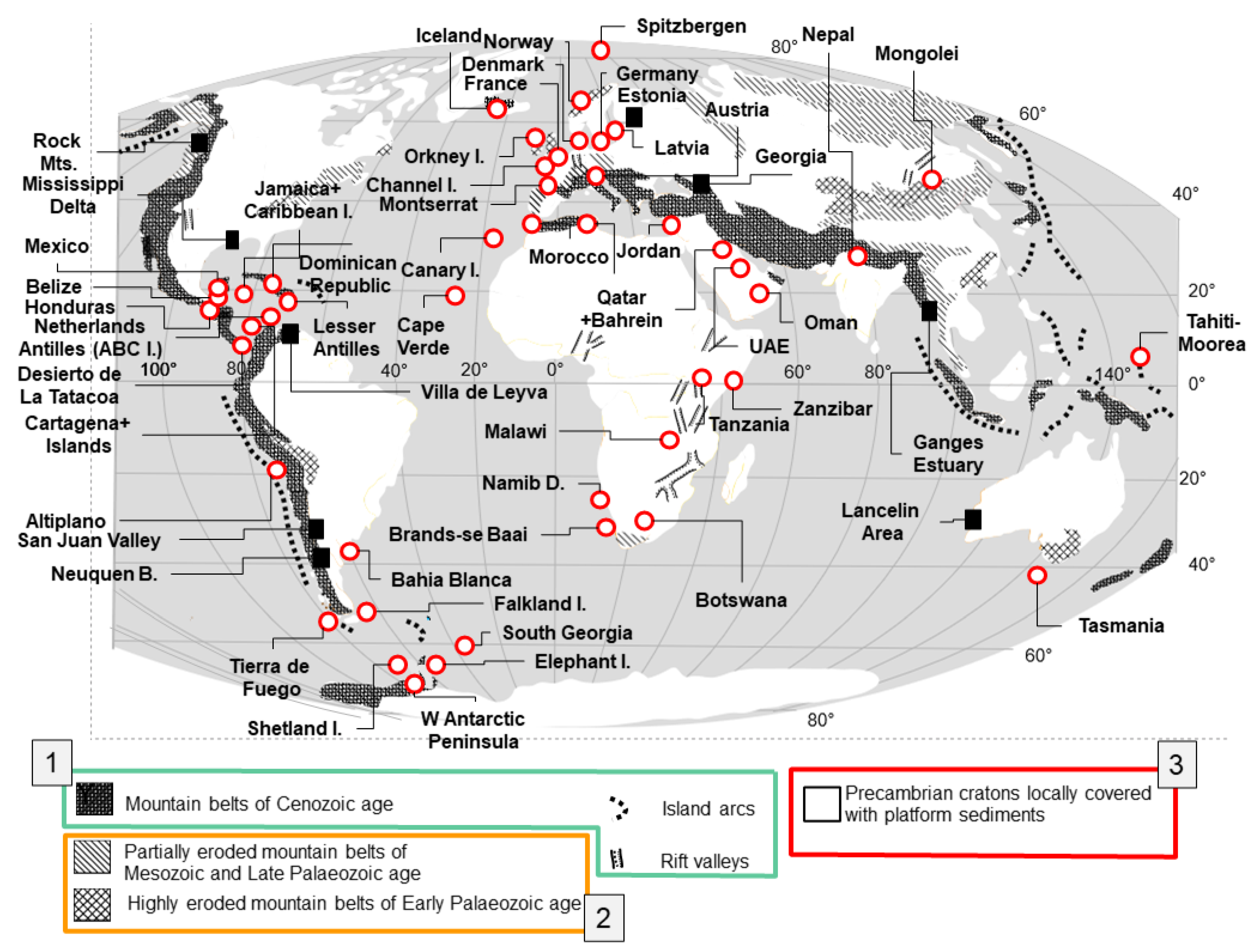
  • To determine whether the geological setting (geodynamic setting) has an impact on the datasets of these environments;
  • To bridge the gap between a review and a manual.
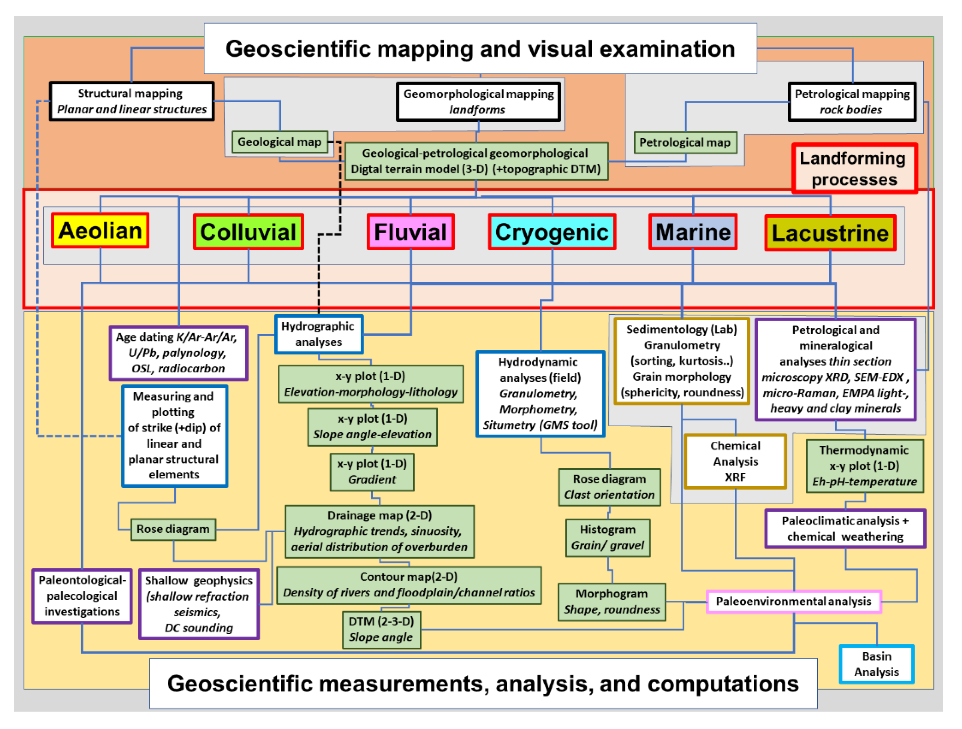
The unconsolidated Quaternary sediments provide ideal reference environments while being in the “statu nascendi” (Figure 1 and Table 1) [34,35].
The current study is basically aimed at applied geoscientists and has been written in a review style, even if the text does not fully comply with the criteria typical of this type of publication, in which data is collected from the literature and a synthesis is formed. The sampling was conducted during a period of almost 40 years on all continents in search of mineral and fossil fuel deposits (coal, radioactive elements) and for environmental geology (finding sites for waste disposals, housing and industrial areas safe to live and work in with regard to geohazards such as flooding and mass wasting, and avoiding conflicts of interests concerning water supply, agriculture and recreation). This is to demonstrate that the current study is also applicable to the E & E issue (extractive and environmental geology). Figure 1 provides an overview of all study areas where these sedimentological, mineralogical and sedimentological studies played an import role in the E & E issue projects and suitable unconsolidated siliceous, calcareous and volcanogenic sediments of Quaternary age could be sampled for the current study [37,38,39,40,41]. Thereby, a homogeneous database regarding analyses and interpretation could be ensured, a fact which is mandatory but could not be attained by collecting data from the literature.
The combination of physical and chemical data necessary to design the graphs in this paper can be used as a reference for different sedimentary processes (mass wasting, fluvial, coastal-marine, aeolian, etc.) operative in the present, but can also be used for stratigraphic series laid down in the geological past provided the diagenetic and metamorphic overprinting is moderate. This methodological assumption draws on the idea of Charles Lyell (“The Present is the key to the Past”), which is widespread among geoscientists and is also a key element in sediment-hosted mineral deposits [42].

2. Methodology

The current review–manual particularly addresses the needs and wants of those working in applied geosciences. As a reference for applied geosciences, economic geology can be used. It is not a discipline of its own, but a “mixtum compositum” of various subjects of earth sciences dedicated to finding new inorganic raw materials and enhancing exploitation of those already known. Geology and mineralogy are the key players in achieving these goals. To these disciplines, I have devoted a review paper [37]. However, there are also other fields which, in some cases, even surpass the aforementioned disciplines, such as sedimentary petrography, sediment chemistry and geomorphology. The author has worked in this subject from 1976 until the present, and places particular emphasis on these three disciplines as a supplement to the mineralogical-geological review published previously [37].
The current study forms part of what was previously called a geoscientific terrain analysis, a methodological flow chart of which is illustrated in Figure 2 (Wilson and Gallant, 2000). In the current review, only the analytical work of the terrain analysis is addressed, and is highlighted in grey, whereas a complete overview of the terrain analysis can be found in [43].
Petrographic microscopy: Routine thin section analysis was carried out in combination with optical microscopy of heavy and light minerals with 200 to 300 grains counted per sample. HM separation was carried out for each sample to the grain size fractions richest in HMs (the 3–4 Ø fraction) using sodium polytungstate of a density of 2.9 g/cm3.
X-ray diffraction analysis: X-ray diffraction (XRD) patterns are a supplement to the aforementioned method and were recorded using a Philips X’Pert PW3710 Θ-2Θ diffractometer (Cu-Kα radiation generated at 40 kV and 40 mA), equipped with a 1° divergence slit, a secondary monochromator, a point detector and a sample changer (sample diameter 28 mm). The samples were investigated from 2° to 80° 2Θ with a step size of 0.02° 2Θ and a measuring time of 3 s per step. For specimen preparation the top loading technique was used.
Electron microscopy: Scanning-electron analyses (SEM-EDX) were conducted by means of a QUANTA 600 FEG equipped with a GEMINI EDX system. Because all analyses were carried out under low-vac-chamber conditions (1 to 10 mbar), no sputter coater was used prior to analysis.
Electron microprobe: The chemical composition of some minerals was analyzed with a JEOLJXA-8530F field emission microprobe which was set to an acceleration voltage of 20 kV and a sample current of 40 nA. For the microchemical analysis of the minerals, different X-ray lines, standards, measuring times, and crystals were used.
CAMSIZER analysis: Grains in the size interval of 63–2000 μm were subjected to a more detailed granulometric and morphometric analysis using the laser-based CAMSIZER analysis. The CAMSIZER® measuring system is based on digital image processing.
X-ray fluorescence analysis: Major and trace elements were analyzed by applying X-ray fluorescence spectrometry (XRF). Samples were prepared by mixing with a flux material and melting into glass beads. The beads are analyzed by wavelength dispersive X-ray fluorescence spectrometry (WD-XRF). To determine loss on ignition (LOI), 1000 mg of sample material was heated to 1030 °C for 10 min.

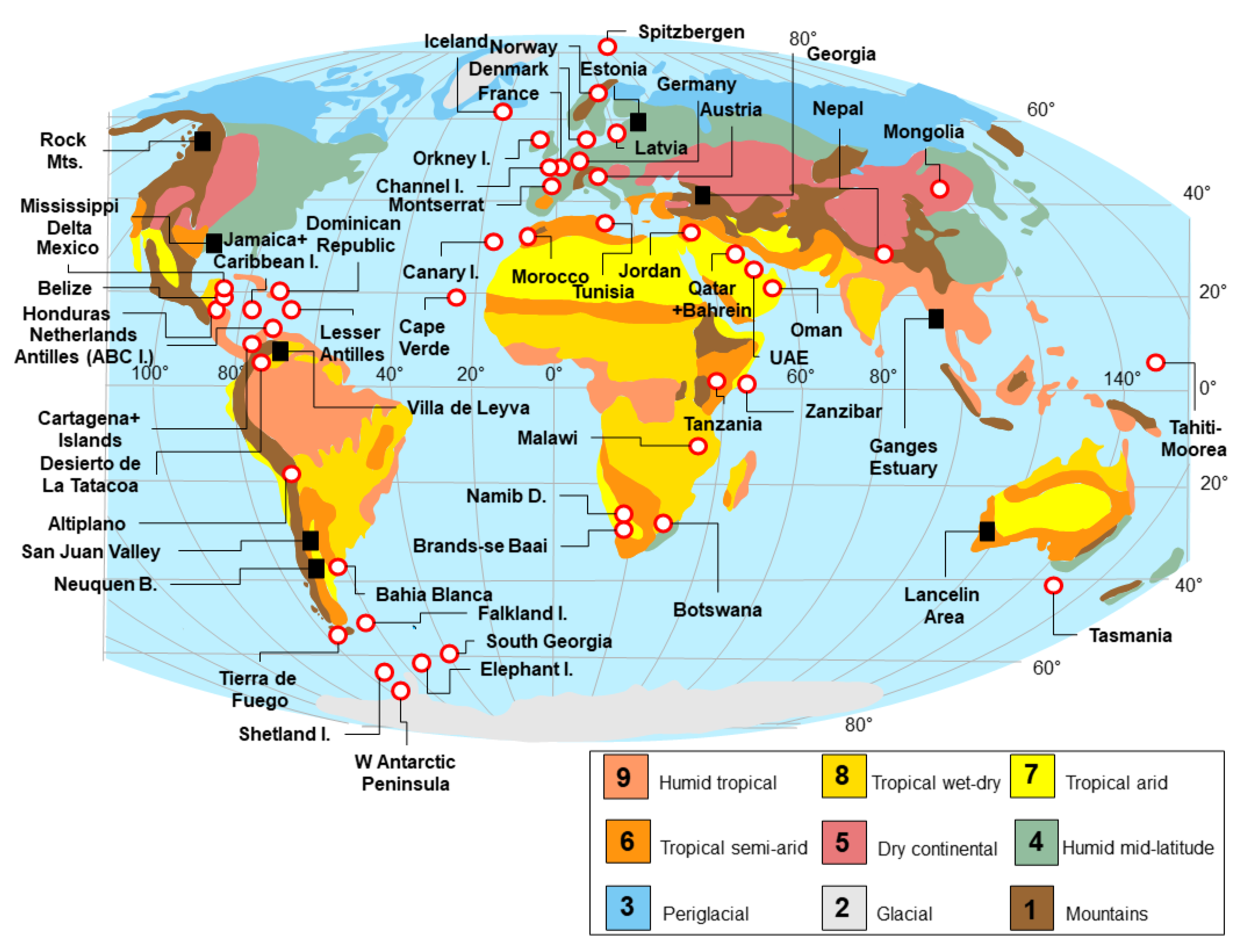
3. Geological and Climatic Settings

The geological settings of the various study sites under consideration are very different from each other. In order to avoid endless descriptions and repetitions that might distract the reader from the essence of the current study, a “common denominator” has to be found. The tripartite geomorphological-geodynamic maturity concept was selected herein to address this issue of finding a common geodynamic platform for discussion (Table 1 and Figure 3) [36]. This connects the small-scale geodynamic setting with the landscape, which is the large-scale host of all land-forming processes addressed in this publication (Table 2, Figure 1 and Figure 3).

3.1. The Pre-Mature Category 1

Category 1 encompasses the mountain belts of Cenozoic age, and the island arcs and elongated grabens and rift basins (Figure 3, Table 1 and Table 2). Mountain belts of Cenozoic age extend along the western edge of North and South America and from the Pyrenees, France–Spain, through to South-East Asia, exemplified by the remarkable plateaus and intramountain basins such as the Altiplano of Bolivia and Peru, the Katmandu basin in Nepal, and the Desierto de la Tatacoa between the Cordillera Central and the Cordillera Oriental of the Andean Orogen [47,48].
Colombia (Figure 3 and Table 1). The tectonic movements responsible for the build-up of these high-altitude mountain chains began during the lower Cretaceous and faded out during the Paleogene with regard to the Alps and a collisional orogen. Subsequently, approximately 45 million years ago, the Himalayas began to develop as the Indian Plate was colliding with the Eurasian Plate [49,50]. The geodynamic setting can be taken as a reference type for the maximum uplift. Excluding some high-altitude plateaus, e.g., Altiplano, deep erosional dissection is the governing factor during the shaping of the landscape and formation of clastic sediments.
Both the continental grabens and island arcs environments share one characteristic feature—they occur as narrow elongated geodynamic zones. Conversely, they are marked by rather contrasting plate motions and are representative of highly mobile stages along well-developed plate margins or plate margins which are still in the making by going through a period of crustal spreading. The intercontinental grabens and the volcanic rocks genetically lined up with them are shown side-by-side along the East-African Rift, from Malawi, through Tanzania to the Red Sea-Jordan Rift (Dead Sea Transform Fault) (Figure 3 and Table 1). Another narrow elongated geodynamic setting of island arcs bounds the various plates in the Caribbean Sea. The Lesser and the Netherlands Antilles, and some islands connecting the southern tip of South America with Antarctica, belong to this geodynamic zone (Figure 3).

3.2. The Mature Category 2

Highly to partially eroded mountain blocks of Paleozoic and Early Mesozoic age, such as the Variscides and Caledonides in Europe, the “continental bridge” between the Falkland Islands and the southern tip of South Africa, belong to this mature category 2. The sedimentary unit underlying much of the Falkland Islands is the siliciclastic Siluro-Carboniferous Gran Malvina Group [51,52]. This is also the case with some Mesozoic orogens in the Central Asian Interior in Mongolia (Figure 3 and Table 2). The Caledonides, covering the Cambrian through the Devonian, represent an orogen, encompassing the Appalachians in North America, North and East Greenland, Spitzbergen, the north-western British Isles and Western Norway, which were separated from each other by the opening of the North Atlantic Ocean [53]. Spitsbergen forms an uplift of the Barents Sea Shelf, the basement rocks of which are Precambrian through Silurian in age. The Early Paleozoic Caledonian orogeny tectonically and metamorphically influenced this study site [54].
The Hercynian (Variscan) orogeny contributed to a significant increase in the landmass on the Northern Hemisphere from the upper Devonian through the Permian [55,56]. The Paleozoic basement areas are relatively deeply dissected as in the Atlas Mountains in Morocco (Figure 3). Another orogeny, the Cimmerian orogeny, left its imprints prevalently in Central and East Asia and was operative in the time span from 200 through 150 Ma; see Mongolian study sites (Figure 3 and Table 2) [57].

3.3. The Super-Mature Category 3

By far the largest area of the globe is occupied by deeply eroded cratons of Precambrian age characterized by shallow to moderately deep dissection. Comparing the climatic zones and the geodynamic setting in Figure 1 and Figure 3, respectively, the basement rocks of the Precambrian cratons are exposed from the pole to the equator and influenced by the climatic processes of all climate zones.

3.4. Landscape Formation and Climate Zonation

The landscape-forming processes of the super-mature category 3 do not operate immediately on the Precambrian magmatic and metamorphic basement rocks (Table 2). From platform sediments of variable thicknesses and age, they carved the landscape out of the Quaternary, topstrata of which are the objects of the current review. This is also valid for the mature category 2 where large Mesozoic epicontinental basins subsided into the Paleozoic Variscan Basement [58]. To a lesser extent, it can also be applied to the modern fold belts of category 1 where Mesozoic to Cenozoic sediments spread across the intramountainous plateaus and foreland basins proximal to the foot slopes of the rising mountain chains, and took up the Cenozoic debris generated by the erosion of the hinterland [59]. Basement and platform sediments were dissected by grabens of category 1 which were filled with Cenozoic sediments and magmatic rocks [60]. In combination with the climate, arranged in discrete climate zones between the poles and the equator, the landscape-forming processes created what is called a morphoclimatic zonation of the Earth surface.
To enhance visibility, the climate zonation applied during the current study and illustrated in Figure 1 follows the proposals of Scotese [35] covering the timespan younger than 2 Ma (Quaternary). A more detailed climatic subdivision can be deduced from the Koeppen Climate Chart where temperature and precipitation on a seasonal basis are used for a fine-tuning of the climate zones [46,61]. In Table 3 and Figure 1 the platform for a climatological correlation of both classification schemes has been performed.

4. Results—Trends and Compositions

Six sedimentary processes known to have shaped the Earth’s surface are addressed in the current review and listed as a function of climate and geomorphological-geodynamic setting (Table 2). The climate according to Scotese [35] forms the basis of the map in Figure 1. For a further fine-tuning, particularly as to the seasonal and annual temperatures and precipitation, the Koeppen-Geiger Classification is recommended [46] (Table 3). In the following subsection a brief overview of their landforms and deposits is presented and a concise interpretation of them carried out so as to understand the trends and composition prior to the discussion in Section 5.

4.1. The Landform Series

The landform series form the platform based upon which the diagrams can be understood and discussed. Their prevailing land-forming processes are briefly described in general and some typical sampling sites of the diagrams are illustrated in more detail and taken as reference for the landform series using the codes in Table 2 and Table 4 for correlation.

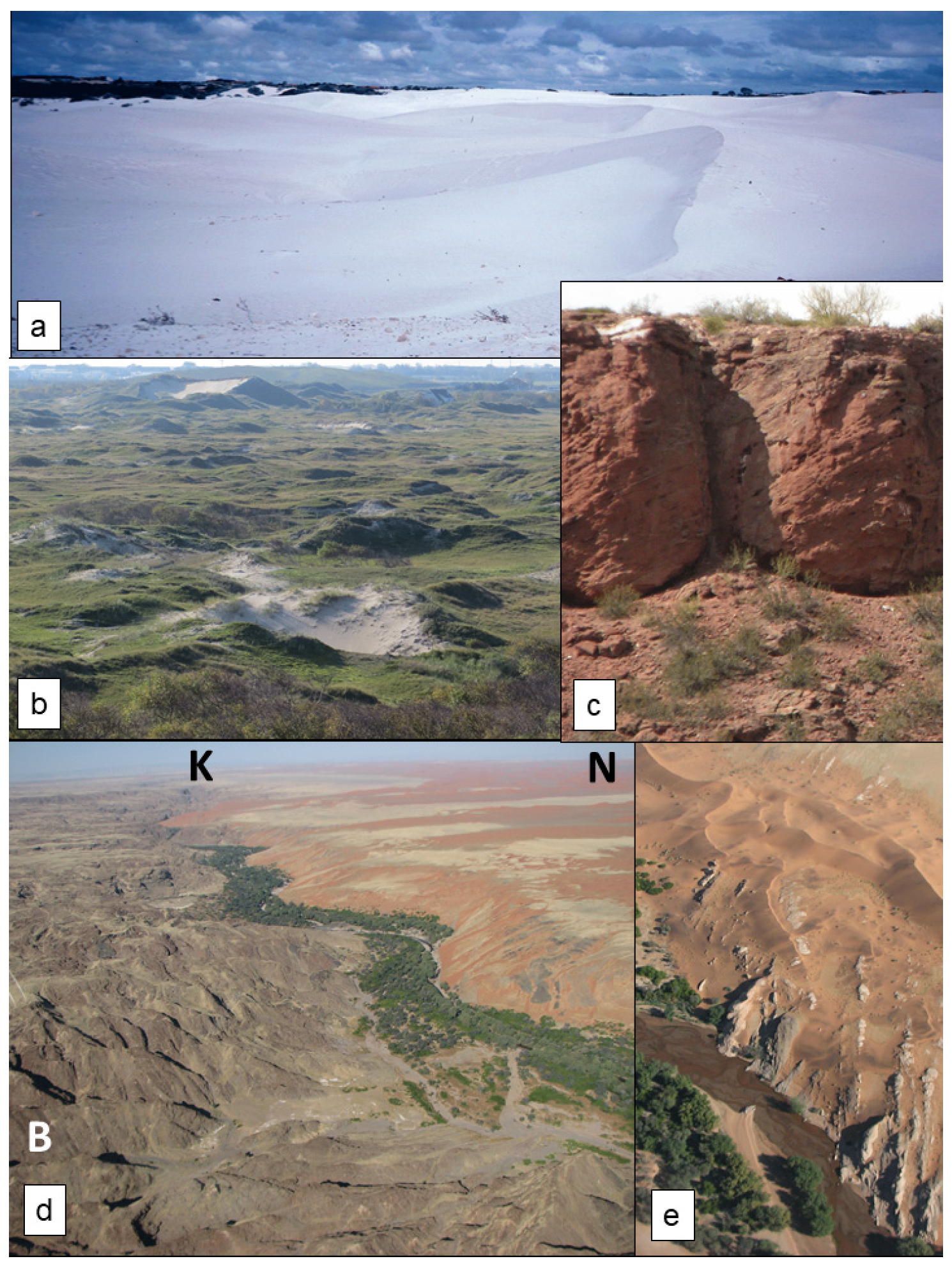
4.1.1. Aeolian Processes and Their Landforms

Erosional landforms of landform series 1 (LFS 1), e.g., ventifacts, mushroom rocks or desert pavement and depositional landforms, e.g., transverse, cliff-front dunes and sand sheets, are formed by means of wind transporting sand-sized particles after being picked up from the deflation areas via suspension, saltation and rolling [62,63,64]. These arenaceous grains are laid down as the wind speed is reduced by bottom roughness, obstacles and increasing wetness. The most recent comprehensive review on the aeolian environments through time has been published by Rodriguez-Lopez et al. [65]. Dill and Buzatu [66] delivered an overview of syngenetic (aeolian placers) and epigenetic mineral deposits in Cenozoic and Permo-Mesozoic host rocks. Many coastal plains such as in the immediate surroundings of Perth, Australia, show shoreline-parallel elongated coastal dunes piled up by the landward blowing wind but are rather stationary and strongly decarbonated by in situ processes. The aeolian depositional landforms grow older towards the hinterland [67,68] (Figure 4a). The depositional and erosional aeolian landforms are listed in Table 4 based on the study sites investigated and sampled for the presented review. The landforms occur in coastal and inland regions and tend to grow bigger in size towards the inland in each of the three maturity categories (maxcoastal: 1 km; maxinland: 1000 km). From the pre-mature, through the mature to the super-mature geomorphological-geodynamic maturity category, the size steadily increases. In the pre-mature category, the depositional zones are controlled by the coastal evolution or by morpho-tectonic depressions in inactive volcanic edifices [69,70]. The aeolian inland landform series often are characterized by a very short distance between deflation and depositional. The inland aeolian landform series exhibit a great variety of landforms indicative of a short-distance wind transport with the same sites acting as sand source and host area, such as wadis in badlands and semi-desert environments [40]. Desert varnish, ventifacts and mushroom rocks and sand sheets developed next to each other.
The super-mature crustal category 3 is the archetype of the aeolian landforms with, e.g., star dunes, barchanoid dunes, parabolic dunes, longitudinal dunes, and transverse dunes in the northern and southern desert belts [65].

4.1.2. Mass Wasting Processes and Their Landforms

Mass wasting, abbreviated to LFS 2, includes all kinds of down-slope movements of debris driven by gravity. Its various subtypes may strongly differ with regard to their velocity and the incorporation of water. When the slurry is soaked with water at the highest wetness rate possible, and hence moves at the fastest rate of particle transport, it turns into what is subsequently treated in this review as a fluvial process [44]. If this gravity-driven mass wasting process works its way downslope at a similar high speed but under almost dry conditions it turns into a rock slide. Those end member-types of mass movement operative under a very dry regime and during very slow motion summarized as par-autochthonous conditions are denominated as heave, a setting also well represented by cryoturbation under cold climatic regimes. Mass movements strongly shape the topography of the Earth’s surface; in combination with fluvial processes, this movement is accountable for the morphology of mountain and valley systems, the quality of rivers, streams and groundwater flow, and the vegetation that covers much of the Earth’s subaerial surface [71]. The slowest motion easily recognized in the field under rather dry (talus) and wet (soil) conditions is creep resulting in lobes and multiple series of step-wise terracettes (Figure 5a). This may be found on all slopes of fluvial drainage systems provided there are loose debris or soil. In the succeeding sections, a subdivision into slow motion and fast-motion mass wasting is consequently conducted (Table 4).
Mass wasting includes some missing links to the cryogenic land-forming processes addressed in 4.3 [72,73,74]. A great deal of mass wasting goes downslope much faster and gives rise either to flow deposits when enriched with water, which acts as some kind of lubricant, and slides under drier conditions (Figure 5b–d). Mass flows and debris flows resemble true fluvial deposits in terms of roundness and landforms such as levees, channel braiding and their incision rates (Figure 5b,c) [75,76]. Similar to the previous aeolian processes, there are also two principal subgroups: (1) depositional landforms (Figure 5a–d); and (2) erosional landforms (Figure 5e–h and Table 4). The granitic tors and woolsacks summarized under the header monadnocks are autochthonous, first reflecting the base of the regolith and, second, when exposed, marking the undulous topography of the former peneplain (Figure 5f,g). Some collapsed through time and their tilted sliding blocks gradually formed block meers and block streams [40,77,78]. In a granitic landscape, the boulders of the tors, talus, and blockfields frequently have characteristic surface expressions such as tafoni and oricangas, which are often markers of the Pre-Quaternary warm climatic regimes during regolititization described by different Neogene models on Aruba Island by Sumner and Meiklejohn [79].

4.1.3. Cryogenic Processes and Their Landforms

The cryogenic LFS 3 also consists of a great variety of landforms, some of which, due to limited access in the marine realm, are represented to a minor extent in the sampling campaigns for the current study. Glaciers and ice fields hide a great deal of the landforms and expose the ground moraine and kames moraine, and their grinding tracks (whalebacks, roches moutonnees) in the landscape only when on the retreat or when they have completely disappeared (Figure 6a,g). Menzies [80] delineated the area affected by the ice and snow of the glacier. Glacial geomorphology and the linked equivalent sedimentological, chemical and mineralogical studies focus on landforms in front of, beneath and along the edge of valley glaciers, ice sheets and other ice masses on land and ocean basins. The modern glaciomarine environments and sediments as defined by Domack and Powel [81] have to be excluded in this review when the Quaternary sediments are addressed, in addition to the concentration processes of minerals and rocks in various diagrams later in the text. This is also true for those landforms underneath the glacier as long as the glacier is located on the ground moraine, eskers and drumlins, and striae carving the bedrocks [82]. Only fossiliferous forms can be touched and sampled after the retreat of the melting glacier or inland ice sheets of the glacial period in the periglacial area. Even a short glimpse at the map compiled by Lutgens et al. [83] and Scotese [35] reveals that a great deal of the sampling sites in Central and North Europe are mixed-type landforms with relics of cryogenic origin being part of the geomorphological history of this region (Figure 1 and Figure 6e,f) [36,43]. Isolated ice wedges in lower Triassic sandstones filled with debris from creep, and pockets in the bedrock of river channels filled with cryoturbated gravel, are relics typical of the last glacial period in Central Europe that had their center in northern Europe and on local isolated high-altitude summits derived from the uplifted Variscan Basement blocks and in the rising Alpine Mts. [84]. The greatest intersections with regard to the landscape forming processes are encountered between the cryogenic processes and the mass wasting ones treated in Section 4.2. After the deglaciation, such as in cirques (kars), gravity-driven sedimentation starts replacing glacial deposition and erosion [40] (Figure 6b). U-shaped valleys are the most conspicuous remnants of the previous glaciers, which carved the subaerial landscape and, together with glacio-fluvial and cryogenically induced mass wasting, formed the landscape. At a larger scale, this effect is also made visible by the roundness and sphericity of clasts which underwent fluvial abrasion and/or par-autochthonous heave (Figure 6c). Even aeolian abrasion can be discerned by the presence of ventifacts scattered across the talweg laid bare (Figure 6d). The general split into depositional and erosional landforms already mentioned for other geomorphological processes can also be applied for the cryogenic processes and is adopted in 4.4–4.6. In the (peri)glacial climate-morphological zone, mixed-type genetic landforms and clasts that are largely different regarding their granulometry, morphology and situmetry (clast orientation) are common due to the short-distance movement of the ice “telescoped” into each other. Some are also found in the same site as pattern grounds which downslope grade from in situ heave-induced landforms into lobes of solifluction/gelifluction [85,86,87,88,89]. Their distinction is frequently only possible based on a meticulous investigation of the aforementioned sedimentological parameters such as sorting and roundness (see diagrams).

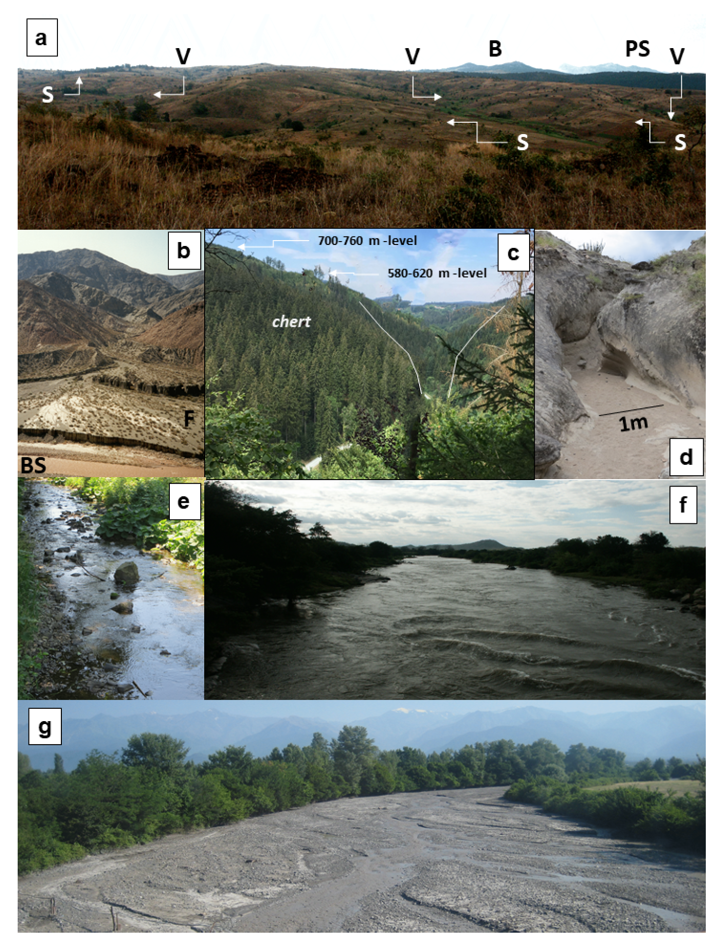
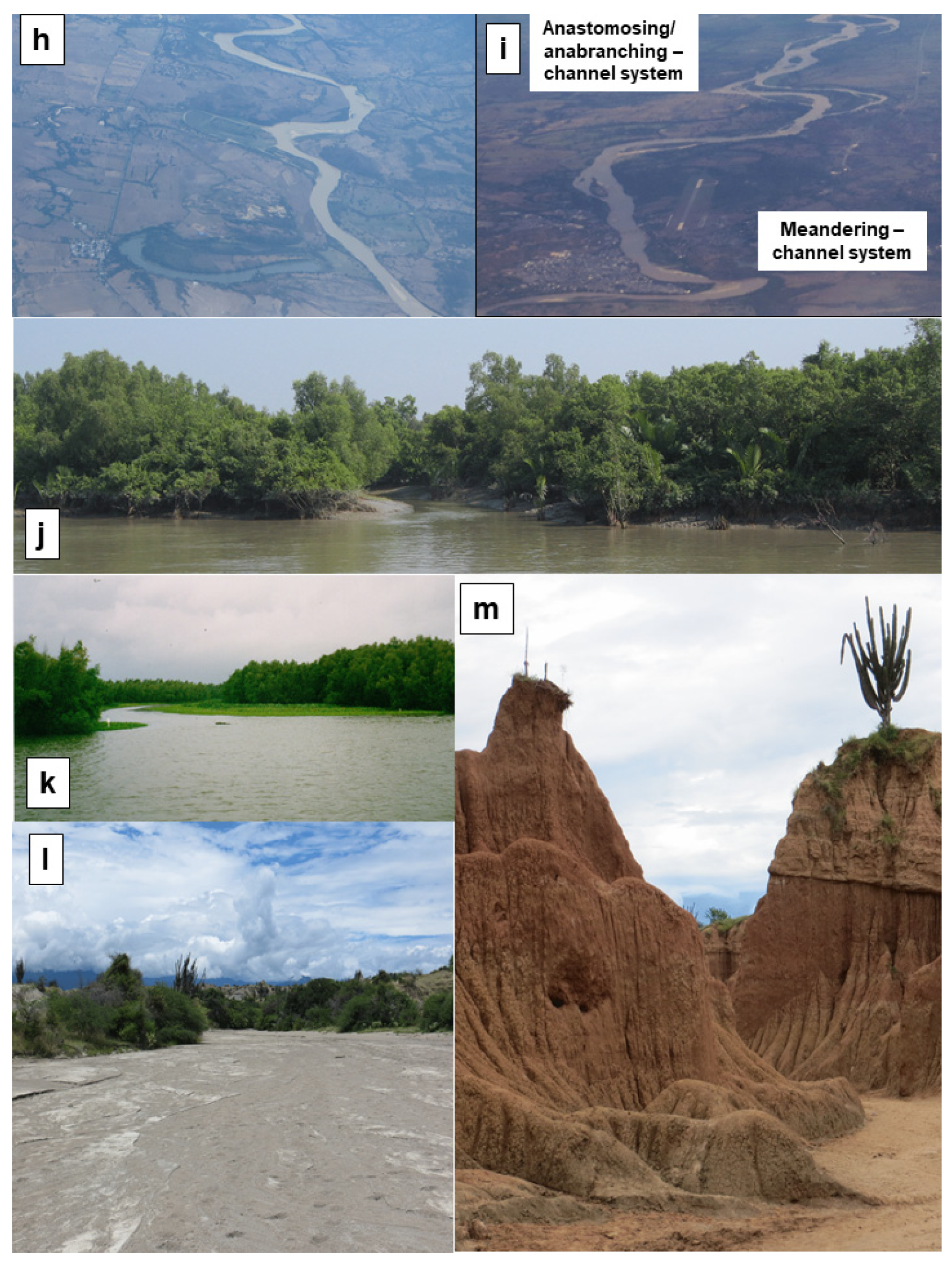
4.1.4. Fluvial Processes and Their Landforms

Excluding the areas permanently covered by glaciers in mountainous and polar regions where H2O is present only in its solid state, fluvial drainage systems are met in all morpho-climatic zones around the globe (Figure 1). Not surprisingly, a wealth of studies has centered around these aquatic land-forming processes and their deposits, of which only a small fraction can be cited here (Table 4) [6,25,31,33,90,91,92,93,94,95]. Different attempts have been made to tackle problems of the fluvial drainage systems of LFS 4. There is common consensus on the subdivision of the drainage systems listed in this section: coarse-grained braided and fine-grained anastomosing channel systems; high-sinuosity coarse- and fine-grained -meandering channel systems; straight to low-sinuosity drainage systems (Table 4) [31,33,90,93,94,96,97,98,99,100]. In additions to these basic types, there are also some more subtle classification schemes that also pay attention to mixed-type fluvial drainage systems such as anabranching, a great deal of which stands out due to its wide longitudinal bars developing into lozenge-shaped vegetated islands sensu Nanson and Knighton [27] and North et al. [101]. The above drainage systems are the backbone of the classification scheme applied to the various diagrams in the current study with some supplements concerning the flow confinement; the persistence of the water flow; and transition into the final depocenter. More than in any other processes that sculpture the landscape, a marked difference can be observed along the river run or talweg. Expressed by the channel gradient and the slope angle, a subdivision into three facies zones can be achieved downstream: CA (zone of headwaters or catchment), TA (transport area) and DA (deposition area). They can be used for all drainage systems under consideration irrespective of the grain fabric and composition.
Headwater zone: The upper reaches of a fluvial drainage system near its source are called headwaters. They are separated from other fluvial catchment areas by a watershed and were established in a pre-existing landscape sculptured by fluvial and mass wasting processes leading to two end-member types (1) a plain type and (2) mountain type. They are often coupled with relic landforms that developed under completely different climates and sometimes different states of geomorphological-geodynamic maturity [43,102].
The plain type is genetically bound to a planation surface that approximates a gently undulating plain with no pronounced features of relief, excluding some isolated bornhardts or inselbergs and escarpments at the margin which may grade into piedmont-surfaces arranged in a staircase-like manner [103,104,105]. It is fluvial in essence, as shown by the shallow valleys and moderately high swells (Figure 7a). The formation of this landscape is still under dispute and marked by three different types of plains, each representative of a different model of landform development: (1) peneplanation (Davis’ theory); (2) pediplanation (Penck’ s theory); (3) etchplanation (Wayland’s theory) [106,107]. These fluvial relic landforms in the headwater zone are representative of the super-mature to mature categories which formed under a tropical wet and dry climate. The wide-angle valleys are dominated by unconfined sheet-floods and ephemeral streams such as the Kuiseb (Figure 7a) [108]. Renewed incision starts with dendritic multiple or single channels straight to low-sinuosity drainage systems when the area becomes uplifted or a more humid climatic regime comes into existence [43].
The mountain type is characterized by alluvial fans in depositional environments with a strong gradient. On one side, it ends in a fan apex high up in a strongly uplifted mountainous terrain and, on the opposite side, the predominantly coarse-grained sediments spread across a leveled landscape or merge with the coarse-grained deposits of braided streams [109] (Figure 7b). The very narrow precipices within the swiftly-rising mountain ranges neither favor a weathering mantle nor soils to creep on the steep slopes, but if laid bare are formed by rapid mass wasting such as rock fall and debris flows. The erosive landforms of the pediments in front of the mountains are followed downstream by the alluvial outwash plain. Dependent on the humidity, these wedge-shaped landforms are scarcely or non-vegetated under arid climates. This is particularly valid for the active channels debouching their gravel into the transport zone of the rivers in the foreland basin of the rising mountain chain (Figure 7b). Zones of particularly high wetness, where water is seeping in the form of a “wet band” in the fans, are called Fontanelli Zones [110].
Transport Zone: This zone of the fluvial system covers a great variety of channel patterns that differ with regard to channel morphology and grain size distribution as a function of sediment caliber, sediment supply, gradient and channel stability [111]. The incision of a non-alluvial acute-angle single-channel (slope angle 30° → 35°, talweg angle 2.7° → 0.7°) of the Wilde Rodach River, Germany, into the Neogene peneplain is displayed in Figure 7c [43]). The abandoned flood plains and erosional terraces at two different levels at different altitudes a.m.s.l. are mapped and interpreted as relics of a large-and-shallow drainage topography. The succeeding V-shaped valley and its sediments evolved under periglacial to mid-latitude temperate climates during the Pleistocene. The non-alluvial straight channels of the Wilde Rodach River are bounded by Lower Carboniferous greywackes and slates. These lithologies provoke a high bedforms roughness and their debris eroded from the channel floor are concentrated in sidebars (Figure 7e). A high channel gradient, sediment supply and sediment caliper are accountable for the step-pools and cascades, and the high gravel and boulder contents.
In the badlands of the Desierto de la Tatacoa, straight to low-sinuosity gullies cut into Miocene sediments of an intramountain basin of the Colombian Andes under tropical wet-and-dry and mountainous climates during the Quaternary (Figure 7d) [41]. Gullying is a widespread process at the passage from headwaters into the transport zone when the substrate of the drainage system is destabilized in terms of bedrock stability (alternating argillaceous and arenaceous sediments) or by structural disturbances such as neotectonics in mobile fold belts [112]. The gullies of type 4.3 pass downstream into ephemeral wide channels (arroyos) of type 4.5. In the Central African Savannah under tropical wet-and-dry climates, the large-and-shallow valleys of the peneplain run into low-sinuosity streams such as the Shire River (Figure 7g) [113]. The different external expressions of straight to low-sinuosity rivers is immediately related to the state of the geomorphological-geodynamic maturity (category 1 vs. category 3).
Coarse-grained braided streams may come up near the mountain ridges as shown by the Turcanray River, Georgia, in front of the Higher Caucasus under dry continental to mountainous climatic conditions (Figure 7g). Why do, in places, these coarse-grained braided streams characterized by gravel-enriched longitudinal bars come into existence whereas elsewhere coarse-grained meandering streams with point bars develop? [102]. Braided streams’ drainage systems exist proximal to the source area where a high stream gradient and an abundant supply of coarse-grained material laid down by periodical unconfined (flash) floods can be guaranteed [33,95,114]. Deleterious to the evolution of braided streams is the lack of accommodation space enabling a vast braid plain to develop and the resistance to significant bank erodibility of dip and strike streams. Anabranching gravelly and mixed-load wandering channel systems have been recorded from vast plains of Northern Australia and the Cape Province, South Africa, but not from Central Europe [96]. The fine-grained meandering stream, exemplified by the Rio Magdalena grade downstream, as the gradient lowers into a river system, is called anastomosing (Figure 7h,i).
Deposition Zone: Fluvio-deltaic landforms and their most fine-grained sediments bridge the gap between the transportation and deposition zones (Figure 7j,k). The most striking subtypes occur at the river mouth as drainage systems enter the sea. In a tide-dominated coastal region such as Bangladesh, funnel-shaped estuaries bounded by mangrove swamps exist (Figure 7j). In a microtidal fluvial-dominated delta regime, a bird-foot delta evolves instead as a consequence of the fluvial power that is active far into the sea. This can be deduced from the typical environmental features of a river, such as the levees and splay deposits opening into interdistributary bays, such as salt marshes and shallow lagoons on the lower delta plain that is already influenced by the sea (Figure 7k).
On dry land such as the Desierto de la Tatacoa, Colombia, ephemeral rivers (wadi) occur that are both source and deposition area, and a mesa-and-butte topography with hill wash plains between them (Figure 7l,m).

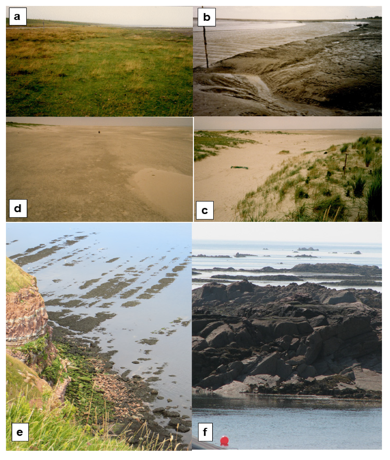
4.1.5. Coastal-Marine Processes and Their Landforms

Many attempts have also been made to classify coastal-marine settings (LFS 5) and characterize their features using physical, biological and geomorphological properties or the mode of evolution, as summarized by Finkl [115]. Briefly reviewing these various attempts of subdivision and description reveals that every researcher swiftly ends up in an enormous amount of different data which may be helpful for detailed investigations of a special coastal issue but which hampers any reasonable comparison of terrigenous landform-series from land to sea as they are listed in Table 4. The hydrographic parameter tidal range is an appropriate measure and a reasonable compromise to categorize the coastal-marine zone, particularly in view of the availability of numerical data on a worldwide basis for classification [116,117,118,119,120]. Moreover, these data directly translate into a rough scheme of coastal landscapes based upon the ground-breaking studies of Davies [121] and Hayes [122], extended by Davis and Dalrymple [123] and Hayes and FitzGerald [124]. Consequently, the current subdivision for the landforms and the succeeding diagrams resulted into two types, 5.1 being representative of the macrotidal-tide-dominated and 5.2 of microtidal- wave-dominated coastal-marine environments (Table 4). A more subtle categorization into, e.g., rocky coasts, beach coasts, calcareous coasts or siliceous coasts can be performed and is addressed in the following paragraphs where meaningful, but it cannot be successfully illustrated by the various diagrams of the compositional and trend sections. It is not only the binary hydrographic regime that matters during a description of the coastal landforms but also the state of progradation or transgression of the coastal zone, the strong impact of which on the outward appearance of the coastal landforms was illustrated by Boyd et al. [125].
Macrotidal/tide-dominated coast: The spatial relationship between the seaward shore platform and the landward cliff provides a convenient means to delineate the coastal zone of tide-dominated coastal areas according to Dalrymple [126] and Davis and Dalrymple [123]. This approach also opens up a perspective to integrate coastal features common to wave-dominated coastal areas where the depositional processes are almost nil and erosional ones predominate [127,128]. The Wadden Sea bounding the German Bight from the Netherlands to Denmark is representative of a gently dipping shore platform lacking any prominent cliff, excluding some higher dune belts and coastal scarps along the North Frisian coast. It is the “type contender” depicted by a quadripartite set of images which under progradational and transgressive regimes develop large tidal flats along a linear terrigenous shoreline (Figure 8a–d). It is a meso- to macrotidal (2 to >4 m) coastal environment according to the classification scheme of Hayes [122] and Hayes and FitzGerald [124]. This meso- to macrotidal environment of the German Bight has been investigated by, among others, Flemming and Hertweck [129], Bartholdy et al. [130] and Madsen et al. [131]. The profile along a gently dipping shore platform perpendicular to the coastline starts with the most landward supratidal zone or salt marsh of the sheltered part of a low-relief coast (Figure 8a). Tidal flats passing from the mud flat through the mixed flat into the sand flat at low tide expose meandering 2nd order tidal creeks which flow into the 1st order tidal channel (Figure 8b). Figure 8c allows a view from the hinterland of the barrier island near the back-barrier lagoon (Wadden Sea) through the pass way of a washover fan on its breakthrough through the dune belt. The most seaward part of the barrier island is the supratidal sand flat between the berm and dune belt, which is a part of the shore platform that is only flooded during storm events (Figure 8d).
The reference type of a high-relief tide-dominated coast occurs on the Isle of Helgoland, Germany, not far from the Wadden Sea in the midst of the North Sea (Figure 8e). The emerged rocky island forms the caprock of a salt dome composed in its core of Upper Permian Zechstein evaporites. The steeply plunging cliff was carved out of the Lower Triassic Buntsandstein series, made up of alternating red sandstones and claystones, with a picturesque isolated stack in front of the headland. The rocky tidal flats are characterized by the outcropping edges of the competent sandstone beds at low tide. They are in contact with the steep cliff at a right angle. The recession of the cliff is caused by topple and rock fall leading to talus scree at the foot slope (Figure 8e) [132]. Unlike the red cliff of Helgoland, where only mass wasting products form the link between the two erosional products of cliff and rock flat, at Grouville Bay on the Isle of Jersey, Great Britain, bosselated rocky tidal flats are exposed at low tide [43]. On the moderately dipping shore plane large marine gravel and sand flats occur between stumps on the foreshore, whereas gently inclined bluffs terminate the hinterland seaward (Figure 8f). Sedimentary intertidal flats are rather featureless, whereas the rocky tidal flats sculptured out of the “Coarse-grained SE Granite” are morphologically very different, ranging from stumps to flat humps.
Where point sources of detrital input exist along such tide-dominated terrigenous coasts, they form what is called a funnel-shaped estuary. In the case of the Wadden Sea, this fluvial input occurs at the mouth of the River Elbe. More pronounced than in the German Bight, this fluvial-marine environment is strikingly expressed in the Bay of Bengal (Figure 7j).
Microtidal/wave-dominated coast: Wave-dominated coasts follow what have been referred to as tide-dominated coasts in terms of their landscape, showing the same binary classification scheme of low- and high-relief coasts. The Baltic Sea is known for its wave-dominated coastal areas showing a characteristic coastal-parallel zonation with barrier islands and spits, such as the aeolian-marine Kurian Spit, Lithuania. NE of this outcrop, wave-dominated gently dipping shore platforms extend near Ventspils, Latvia, with berms and runnels close to the waterline (Figure 8g). Further east in Estonia, high-rising cliffs exist near Paldiski where they stand out from the sea level (Figure 8h) [133]. The steep cliff has been carved out of Ordovician limestone as the cliff is in retreat due to topple and rockfall as the waves undercut an ancient plateau marking a former erosional platform. The process is described in more detail by a cross section through a composite high relief-coast on the Isle of Gran Canaria, Canary Islands, Spain. In one part of the coast, the initial stages of erosion by undercutting the vertical cliff are marked by a notch; in another part of the coast next to the aforementioned one, the final stage of this combined action of wave action and mass wasting can be seen in a large wave-cut platform near Arguineguín (Figure 8i). Even far from the mainland, this feature of adjacent low- and high-relief coasts can be encountered in the “Archipélago Rosario- Barú” along the Caribbean Coast of Colombia [132,134]. In the Isla Grande, a narrow strand plain blanketed with bioclastic beach sands and rubble has been cut by the marine surf out of the reef edifice resulting in a cliff coast (Figure 8j). When marine breakers during multiple storm events levelled the reef and finally disintegrated, washover fans flattened the reef carbonates down to the sea level, conducive to the final result of “cays”, an island landform abundant in coralline gravel surrounding a reef or scattered on top of it [135].

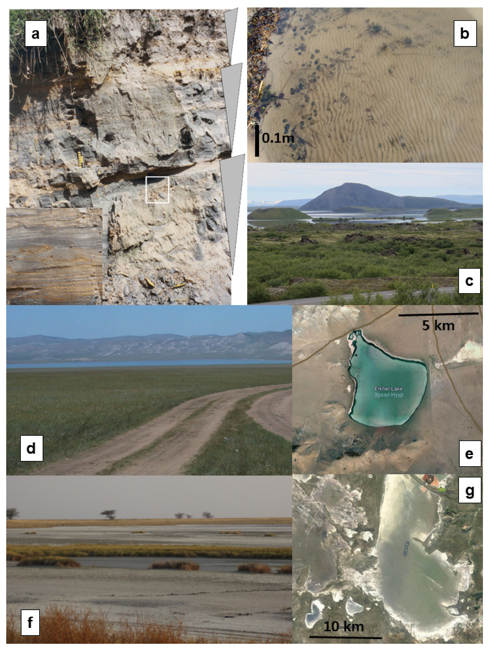
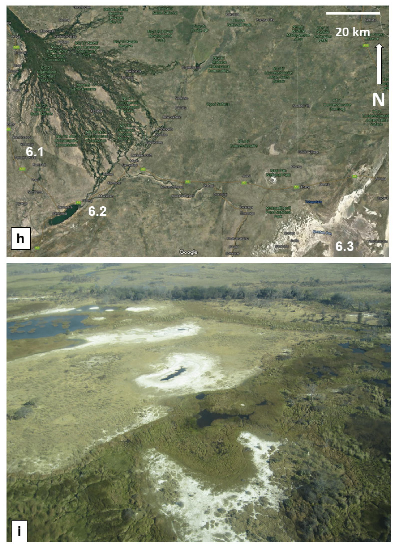
4.1.6. Lacustrine Processes and Their Landforms

Considering geomorphological and sedimentological studies, lacustrine environments (LFS 6) are always slightly eclipsed by the aforementioned ones. The environments addressed previously reach a wider audience in publication than the two basic lacustrine types denominated as perennial and ephemeral lakes (Table 4). The lacustrine type 6.1 mentioned in Table 2 is a transitional type describing lakes in the fluvial environments, such as oxbow and interdeltaic lakes in the marginal lacustrine environment (Figure 9h,i). Regarding the processes responsible for these landforms, the reader is referred to 4.4.
There are a few studies providing an overview of the various types and the prevailing processes to create such standing lacustrine water bodies and their characteristic physical-chemical conditions and biological setting [136,137,138]. In applied geosciences such as the study of sediment-hosted mineral deposits, however, ephemeral lacustrine environments may draw much attention for their evaporite concentration and duricrusts [137,139,140,141,142].
In the following paragraph examples of lacustrine environments are addressed following the pathway from perennial lakes abundant in organic matter, to ephemeral lakes that can be exploited for salt or chemical sediments, in general, where terrigenous sediments still occur but are considerably outnumbered by the amount of evaporites.
The Kathmandu Valley, Nepal, is an intermontane basin in the center of a large syncline of the Lesser Himalayas filled with three units reflecting an alluvial through lacustrine depositional environment during the Pliocene-Pleistocene [143]. This sort of basin has always attracted the attention of economic geologists in search of fossil fuels due to the high TOC values of their basin fill, which is attested to by the dull grey and black rock color of some of their fine-grained clastic sediments hosting either coalified or bituminous matter [136,144,145,146] (Figure 9a,b).
In the Kathmandu Basin coarsening upward (CU) couplets made up of carbonaceous silty mud, laminated mud, bedded silt and fine sand occur in the Kalimatit Facies. Siliceous particles were settling down from suspended load in a standing waterbody forming the distal facies zone of a lacustrine environment. When the wave base was lowered to the sediment-water interface by episodical storms, wave ripples came into existence. In the topmost parts of each CU unit, wave ripples are replaced by current ripples. These structures were derived from microdelta-like distal crevasse splays which discharged their fine-grained sediment load onto the floodplain and marginal lacustrine deposits (central to marginal lacustrine). The organic matter (OM) is composed mainly of little floral remains undergoing different stage of coalification. In the Steinhuder Meer, Germany, the leaves and remains of reeds and branches washed into the lake are almost recent in age, and only in places have reached the state of peat attaining a thickness sufficient for a commercial exploitation (Figure 9b). The longitudinal wave ripples in the fine sand turn landward into bifurcating wave ripples on decreasing water depth and bear witness to the shallow water depth of this peri-glacial perennial lake. It originated from thermo-karst processes during the late glacial period [147]. There exists a wide range of perennial lacustrine environments resulting from endogenous processes. Outstanding examples are found in the volcanic landscape of Iceland. Phreatomagmatic processes created pseudocraters there and sparked the formation of vast lava blankets of plateau basalt surrounding perennial lakes in the environs of Myvatn, Iceland (Figure 9c).
The sequence of photographs and satellite images (source: Google Maps) shown in Figure 9d–g illustrate the development of ephemeral lakes from a transitional perennial to a full-blown ephemeral lacustrine state. Lake Erkhel, Mongolia, is a typical shallow steppe lake with a wide rim of fine-grained siliciclastic sediments and a narrow rim made up of salt efflorescence (Figure 9d,e). As a result of the intermediate position of steppes between polar and warm deserts, salt efflorescence with gypsum, halite, mirabilite and soda, together with calcretes, came into being [148]. Taking the evaporation to the extreme closer to the equator will cause shallow salt pans to come into existence, as exemplified by the Sua Salt Pan, Botswana, in the African savannah, where a broad rim of duricrusts surrounds patchy salt encrustation of a central facies (Figure 9f,g) [149]. It is a multi-type Holocene to Late Pleistocene ephemeral lake with a variegated mineral assemblage of light (quartz/chalcedony, feldspar, analcime, clinoptilolite, calcite, kaolinite/halloysite, illite-smectite mixed-layers, halite) and HMs (baryte, clinozoisite-epidote s.s.s., amphibole, corundum, tourmaline, geikelite-enriched ilmenite, rutile, sphene, kyanite, andalusite, staurolite, garnet, zircon, apatite, monazite, cassiterite, garnet, biotite) [150]. The multitype character is underscored by the adjacency of (1) sulcrete-silcretes, (2) silcretes, (3) calcretes and (4) halcretes (soda ash). The salt pans are fed through ephemeral streams and inland deltas such as the Okawango Delta. The highest degree of evaporation is indicated by the precipitation of potash salt in the Pliocene Sedom Lagoon of the Dead Sea Rift, Israel [151]. The ephemeral lacustrine environment of LFS 6 concludes this six-landform series from LFS 1 to LFS 6. This series forms the platform for the mineralogy and its photo succession of HM (Figure 10), the diagrams showing the various trends (Figure 11, Figure 12 and Figure 13) and the chemical compositions (Figure 14). These fine-grained well-sorted lacustrine sediments of LFS 6 are one of the most common deflation areas of the aeolian processes (LFS 1) when becoming dry (Table 4).

4.1.7. Pedology—From the Ephemeral Lacustrine Environment to the Chemical Sediments—The Issue of Physical-Chemical Markers

The lacustrine sedimentary deposits addressed in Section 4.1.6 bridge the gap into the topstratum of most of the sediments under study, i.e., the soil. Pedological evidence of regression and expansion reflected in the lake sediments and resultant strandlines could be achieved for the late Quaternary of the shore zone of Lake Urmia, Iran [152]. Unlike the sediments under consideration in Section 4.1, this unconsolidated in situ accumulation of minerals not only contains organic but also living matter, which renders it relevant for the growth of plants and trees. The soil-forming processes create what is called the pedosphere at the interface between atmosphere, lithosphere and hydrosphere, and contribute to the persistence of the biosphere gradually evolving from the pedosphere, whereas the lower limit is drawn where the living matter gradually disappears from this topstratum and the lithosphere begins, following textbooks on chemical residues and classification schemes adopted in soil science [139,140,141,153,154]. The interrelationship between the substrate, whether sedimentary, magmatic or metamorphic, and soil-forming processes that also play a significant part in the generation of orecretes s. l., can be deduced from various comprehensive studies [155,156,157,158]. Soil types may be very different as to their organic matter, as shown by a joint geomorphological-sedimentological-pedological study along a transect from the northern Sahara Desert to the coastal zone in NW Africa [39]. In a sequence of photographs running the gamut from soil types, through duricrusts into orecretes, the change of the physical-chemical regime is accounted for and the interrelationship between environmental and economic geology (“E & E issue”) on one side and the sedimentary deposits, in general, and their topmost strata, in particular, is addressed. In this way, support is not only lent to the scope of this joint review-manual—see the Introduction section—but the peer group is also clearly delineated, which lies in a frontier area between genetic and applied geosciences.
Mollic and stagnic vertisol and rubic arenosol on fluvial-alluvial sediments with a strong aeolian influence at the edge of this facies may have more than 3 wt.% OM over the entire soil profile or confined to the upper litter-bearing horizon, respectively, whereas a vertic and luvic planosol on coastal-marine sediments of a microtidal wave-dominated environment (grading laterally and landward into the aforementioned sediments) barely reaches a level of as much as 0.8 wt.% OM (Figure 9j–l). They mirror a gradual but steady increase in the oxidizing conditions in the soil types from the poorly aerated ground water-induced pedons towards the well-aerated pedons near the coastal-marine zone.
A further increase in Eh is signaled by the Quaternary duricrusts, which are almost barren regarding OM and come into being under strongly oxidizing conditions (Figure 9m–o). The example of Figure 9m is indicative of still-reducing conditions, although with an increase in alkalinity of the pore solutions at the boundary between the lower phreatic and upper vadose groundwater zone. In the following setting, strongly oxidizing conditions can be deduced from the selenite modification of gypsum in the Tunisian sabkha (Figure 9n). The mixed-type carbo-vanadocrete is representative of a complex oxidizing environment, although with a reducing source (Figure 9o). This assumption is corroborated by the uranyl vanadate strelkinite [Na2(UO2)2V2O8·6H2O], which has been derived from a stable tetravalent uranium source under a reducing condition where vanadium is a marker mineral. This paves the way into the true orecretes of copper and uranium-bearing APS minerals [159], both of which denote the transition from a reducing primary into a secondary oxidizing environment under a rather acidic regime in what is called a gossan [160].
In general, the in situ topstratum of sediments covering the full range from soil to orecretes contains a great variety of marker mineral and mineral associations, which, in combination with the organic matter, enable the geoscientists to determine the short-term physical-chemical regime at the interface of various crustal spheres. Similar marker minerals and the association encountered within the sedimentary units themselves act in the same way but are cast into the role of long-term physical-chemical markers—see x-y plots later in this study.

4.2. Trend and Compositional Diagrams of Landform Series

4.2.1. The Mineral Assemblages of the Landform Series and Their Sediments

Skimming Section 4.1.6 about the lacustrine landform series LFS 6 may give the reader a rough idea of how variegated the mineralogy of the sedimentary rocks encountered in the different landform series might be. In the trend diagrams, one parameter was derived from the sedimentology, e.g., sorting, whereas the other is related to the mineralogical association, e.g., HMs, or the chemical composition, SiO2. The latter compositional part of the sediments is governed by the quantity and quality of the series of light minerals (LM) (chloride, feldspar, silica, Ca-Mg carbonate, Ca-Mg sulfate, zeolite, white mica, and clay minerals of the kaolinite- and smectite-group). Siliceous and carbonate species are by far the most frequent mineralogical components and used to show an antithetic correlation in the sediments under study. The HMs in the sediments can be categorized into different mineral groups and solid-solution-series (s.s.s.): alumo-silicate group, alumo-oxide group, amphibole s.s.s., Fe-(Mg) chlorite s.s.s., clinozoisite-epidote s.s.s., Fe sulfides, sulfates and Fe-Mn carbonates, Fe-Ti oxides, garnet s.s.s., dark micas, olivine s.s.s., phosphate group, pyroxene s.s.s., Ti silicates, spinel s.s.s., staurolite tourmaline s.s.s., and zircon. Even (semi) opaque ore minerals grouped as Sn-W-Nb-Ta oxides, Bi-As-Sb sulfides, gold, PGM and Pb-Zn-Hg sulfides can be seen in all landform series. To list them all and quote their sources would go far beyond the current review and would cause an overload in the mineralogical literature. The only logical and economic approach to be taken is giving reference to one of the mineralogical databases, e.g., Mindat.org. for further reading. Moreover, in these Quaternary sediments, anthropogenic “minerals” also occur, such as wuestite or pure fayalite, which result from smelting operations of our ancestors. The landforms contain the full range of labile to ultrastable HMs and a great variety of LMs also found in the list of weathering stability [161]. These detrital minerals can not only be used for provenance analysis but their granulometric data and grain morphology also constitute a reliable tool to decipher their mode of transport [66] (Figure 10). Two common HM groups—the (semi)opaque Fe-Ti oxides and the transparent amphibole s.s.s.—are selected in the current review to exemplify how to use these “heavies” as marker minerals for environmental and hydrodynamic purposes. Their outward appearance is of assistance to constrain the source rock, the physical-chemical regime in terms of Eh and pH, and the intensity of attrition during transport in the different depositional environments. This is due to the widespread occurrence in the rocks and the intermediate position that amphibole s.s.s. and Fe-Ti oxides occupy in the various stability charts [161,162].
The Fe-Ti system is rather complex due to the fact that Fe is present in nature in a trivalent and bivalent state and consequently has to be reviewed in a ternary plot together with Ti [163]. In nature, the system is subdivided into some pure oxides at the vertices of the triangle (1, 2, 3) and some s.s.s. along the sides and tie-lines of the triangle (4, 5, 6): (1) Titanium dioxides (rutile, brookite, anatase); (2) magnetite; (3) hematite (goethite, lepidocrocite); (4) pseudobrookite-ferropseudobrookite-pseudorutile series; (5) titanohematites-titanomagnetites; and (6) ulvöspinel and the rare hydrated oxide kleberite (Fe2+Ti6O13•4(H2O)) [164]. The latter is certainly not a simple low-temperature weathering product as attested to by the presence of bivalent Fe. The common final decomposition product in the course of supergene alteration is a mixture of pseudorutile, goethite, and anatase or brookite named “leucoxene” [165] (Figure 10a,b). Ilmenite is quickly rounded by the marine wave action and altered into “leucoxene” (Figure 10a). Only platy squares of anatase are markers for supergene alteration, whereas bi-pyramidal XX occur under hypogene alteration (Figure 10b). The primary minerals titanomagnetite and ulvöspinel, and titanohematites, are redox markers, attesting to reducing and oxidizing conditions, respectively. The quadripartite micrograph sequence of ilmenite shows different morphologies and grain surfaces that enable researchers to constrain the aeolian, fluvial and marine attrition of these Fe-Ti grains during transport (Figure 10c–f). The classical paper dealing with the shaping of detrital grains during transport was published by Dietz [166].
Amphibole is a labile to intermediate mineral, and is ranked third behind olivine and pyroxene in the order of stability against weathering, in chemical terms, against acidic meteoric solutions [161,162]. The stability of this mineral s.s.s. against intrastratal solutions or more basic fluids plays a decisive role during deep burial but is of lesser importance for the Quaternary sediments subjected to supergene alteration phenomena. In view of this high sensitivity reflected by the shape, the cited examples of grain morphologies of amphibole find a plausible explanation in context with the mode of transport of amphibole s.s.s. (Figure 10).
The subangular to subrounded tschermakitic hornblende from beach placer deposits in the Chipoka-Salima District, Malawi, form part of a wave-dominated delta in a lacustrine environment where this silicate co-exists with well-rounded ilmenite from a nearby source area (Figure 10g) [167]. The “roundness” still provides a hint about the mode of transport, whereas the skeletal outward appearance and corroded surface did not originate from lacustrine wave action, but are a relic of tropical weathering, which is common to this Central African savannah. The armored amphibole of Figure 10h is located in the Huelva coastal–estuarine system which opens up towards the Gulf of Cadiz, Spain, in front of the Iberian Pyrite Belt [168,169,170,171]. The macrotidal coastal–estuarine reference system is characterized by a net of braided-river channels with gravel lags in the most landward part. The tidal channels delivered this amphibole from the surrounding rocks into the tidal flats, which are floored by sand and mud [172]. The “limonite” coating denotes a strongly oxidizing regime during deposition in the near-shore environment proximal to one of the largest pyrite-mining districts in the region, which can be made accountable for the in situ enrichment of iron. A similar setting can be recorded from the Isle of Cyprus where Fe and Cu sulfides have been mined since pre-historic times from VMS deposits [173]. This is an angular to very angular aggregate of actinolithic hornblende taken from stream sediments proximal to the mining sites. The morphology reflects a short-distance transport with a strong impact by slow-motion mass wasting (talus creep), as may be deduced from the perfect crystal shape of the magnetite octahedra, the edges of which are unbeveled (Figure 10i).

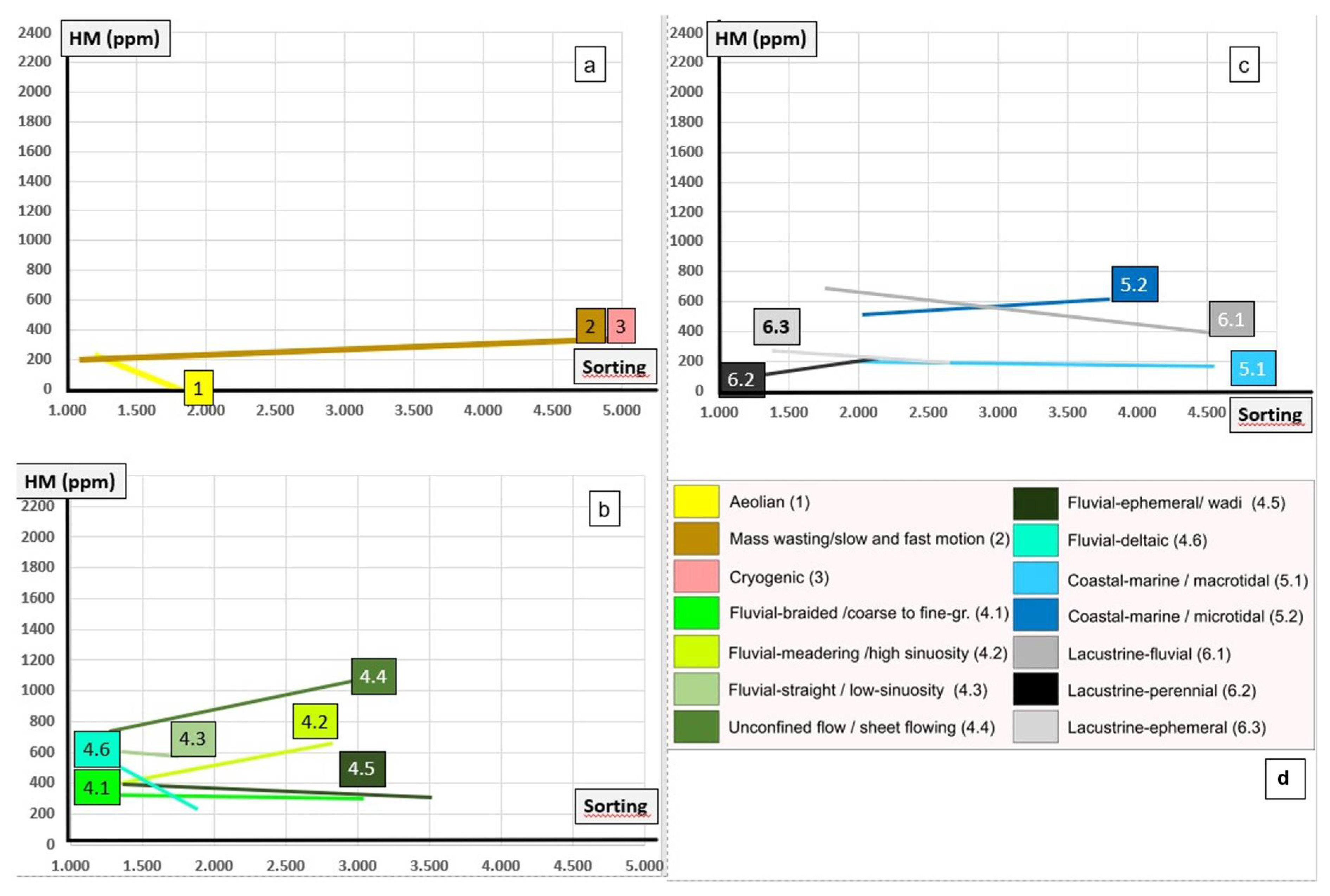
4.2.2. Heavy Mineral Content (Total) vs. Sorting

The x-y plot of Figure 11 connects a textural parameter of a sediment represented by the sorting coefficient along the x-axis with the specific gravity of mineral grains plotted along the y-axis. They form two sides of the same coin, which in this case is the hydrodynamic development in an individual environment of deposition.
The maximum of sorting among the environments under consideration is attained in the pure aeolian sediments due to the constant wind speed and a minimum intervention by other landscape-forming aquatic or gravity-driven processes. The HM contents are as low as those of mass wasting and cryogenic products. This is due to the fact that cryogenic and mass wasting products still contain the majority of HMs in the gravel-size parent lithoclasts and not yet released into the sand fraction. With this in mind, un-reworked LFS 2 and LFS 3 deposits in their most proximal or even in situ position, as is the case with cryogenic deposits, do not contribute much to the arenaceous grain size spectrum of stream sediments (Figure 11a).
This HM scenario conspicuously changes downslope when, after passing into the alluvial-fluvial regime, the landform series are substituted for by the true confined and unconfined drainage systems (Table 4). The sorting improves significantly and the quantities of HM increases (Figure 11b).
The wave-dominated coastal-marine LFS 5.2 and lacustrine LFS 6.2 show the same trend but the marine ones are more effective in the accumulation of HM in their swash and surf zones than the lacustrine equivalent continental ones. [6]. The lacustrine ephemeral and tide-dominated coastal-marine environments are characterized by moderate HM concentration.

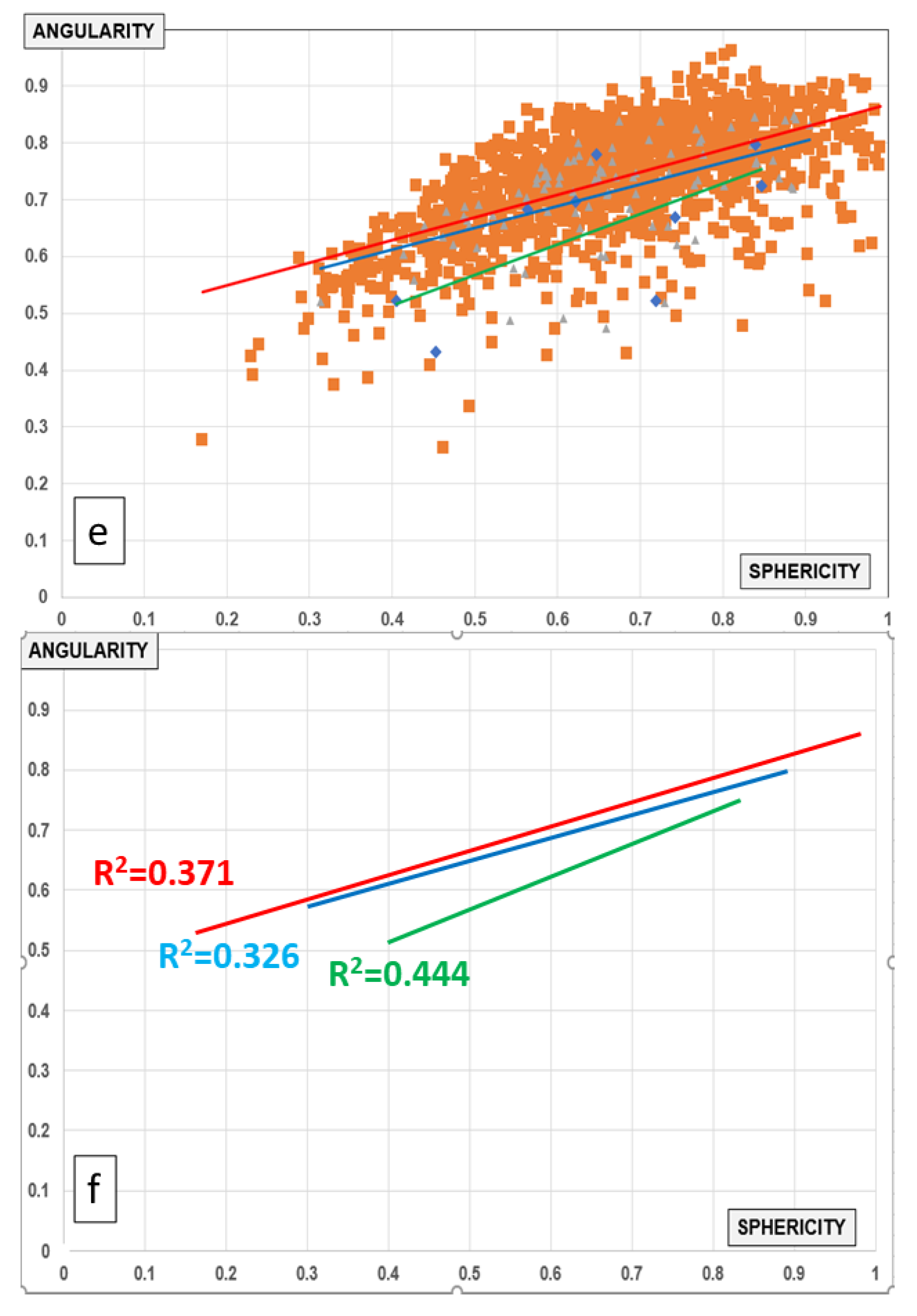
4.2.3. Silica Content vs. Grain Sphericity

In addition to the carbonate content, silica is the major constituent of most sediments. Siliceous minerals are very stable and resistant to attrition, whereas carbonates tend to be very susceptible to dissolution. The mineral grains may have different shapes at the beginning of transport due to their different crystallographic structure and chemical composition. Dependent on the attrition, the means of transport, e.g., rolling or saltation, and the multiple stages of reworking, the mineral grains tend to approximate a sphere in time and space.
Silica in the form of SiO2 is present in a varied group of modifications (low (β) quartz, high (α) quartz, cristobalite, tridymite, amorphous opal). In siliciclastic sediments, and together with Na2O, K2O and CaO, silica makes up the feldspar s.s.s. In sediments there is only one chemical compound, CaO, that rivals the outstanding position of SiO2 and that is accommodated into the lattice of aragonite, and high- and low-Mg calcite; the latter is present in dolomite and its s.s.s. The SiO2 content determined in the sediments under consideration in Figure 12 also yields some kind of a silica/carbonate ratio that is useful later in this review for characterizing the various sediments in more detail from the chemical point of view (Figure 14).
The sphericity is a measure to numerically describe the grain morphology in the sedimentary deposits. It is one of the classical numerical parameters in sedimentology, which has been long used to constrain the mode of transport, and mainly used for gravel-sized siliciclastics [174]. It can be applied in combination with the roundness of grains, which is mostly performed during visual examination using comparison charts [175,176]. The CAMSIZER technique offers a remarkable step forward because it also allows the precise determination of the grain morphology of a finer-grain size spectrum. In addition to the CAMSIZER measurements, the statistics are enhanced by an individual analysis of each mineral grain passing by the laser’s lens. The current approach uses the sphericity of grains measured by means of such a CAMSIZER. When reaching a value close to 100, the grain is close to an ideal sphere. Finally, the sphericity value is plotted in the particle interval 0 to 2000 μm in the x-y plots of Figure 12a–c. It has to be noted that the minimum sphericity has been selected as a reference because the environmental differences of the mean and maximum values tend to be less pronounced than the minimum value and would be less meaningful than the minimum value.
The aeolian, mass wasting and cryogenic sediments under consideration take an intermediate position regarding the silica-carbonate ratio in the trend lines (Figure 12a). With regard to the sphericity values, they are very similar, covering a wide range from 16 to 85.
The fluvial trends form a cluster of trend lines regarding the sphericity and cover a wide interval considering the SiO2 content (Figure 12b). Only the ephemeral streams or wadis stand out due to their trend lines, which display the lowest sphericity determined throughout this sampling campaign.
The lacustrine and marine depositional environments are the final depocenters. With regard to the silica/carbonate ratios, both environments show a rather wide spread. The sphericity territories of both of them significantly differ from each other, with the fluvio-deltaic deposits at the margin of the lakes plotting most closely to their true fluvial counterparts (Figure 12b,c).

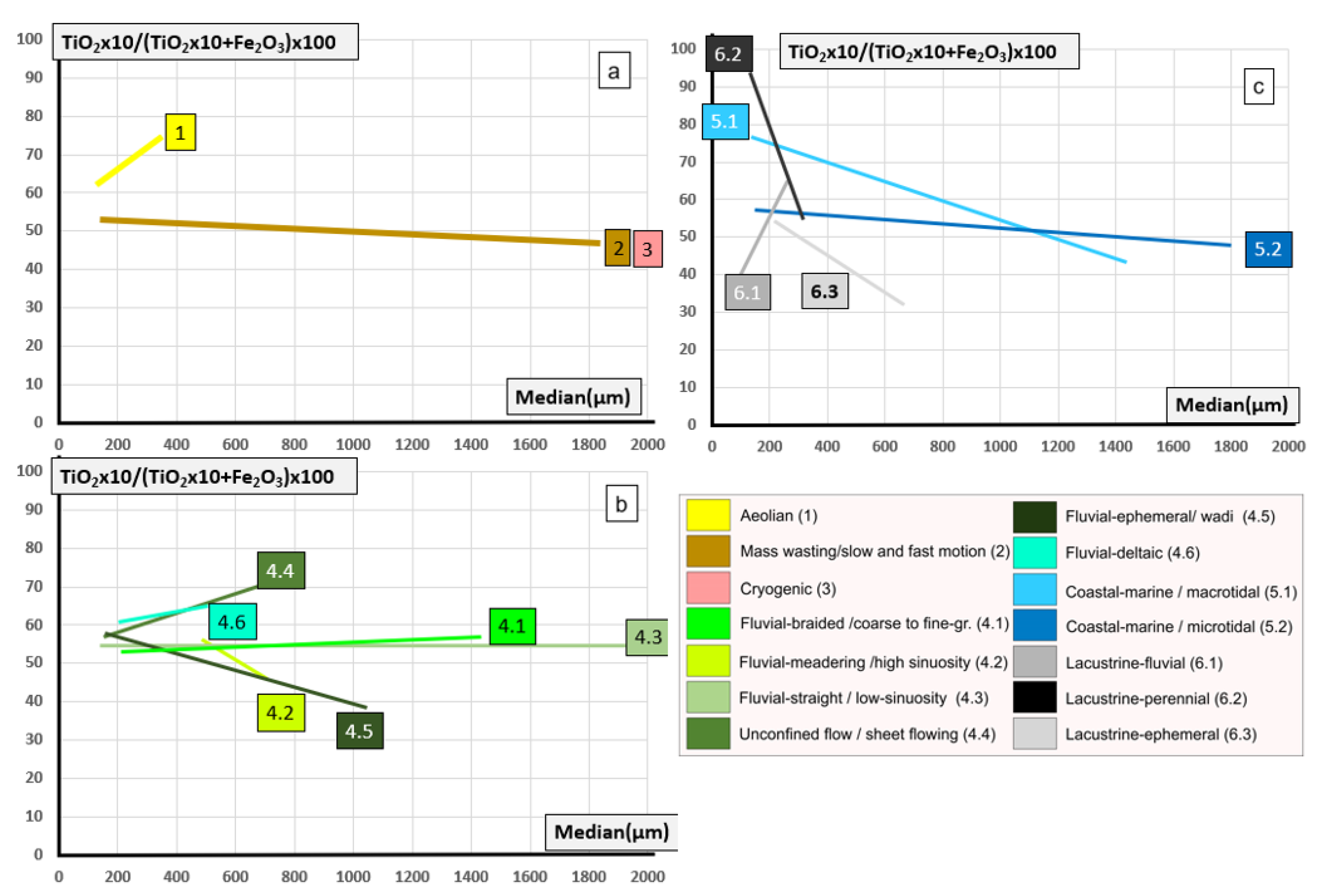
4.2.4. Titanium/Trivalent Iron Ratios vs. Median

Titanium and iron are accommodated in the lattice of many primary Fe-Ti oxides and are found adjacent to each other in silicates as trace elements. “The supergene clock” started running as these host minerals were released from their host rocks and subjected to oxidation at contact with the atmosphere. This strongly affects Fe, but only affects titanium to a minor extent.
By definition, the median is the Q 50 quartile in the cumulative frequency distribution of mineral grains (Figure 13a,b,d). The titanium/iron ratios are chemically a mirror image of what has mineralogically been addressed for the Fe-Ti oxides, underscoring the two valence states of Fe and the monovalent state of Ti. The TiO2 × 10/(TiO2 × 10 + Fe2O3) × 100 ratio has been coined and used together with the Nb/(Nb + TiO2 × 10) ratio to differentiate supergene alteration (weathering) from hypogene/hydrothermal alteration. This was tested on different bedrocks series (metamorphosed ultrabasic, basic magmatic rocks and effusive basic magmatic rocks, linear and areal alteration zones on granites, and on different types of aplites and pegmatites, alteration zones of gneisses and metamorphosed carbonate rocks) [36]. Based on that, increasing ratios of the TiO2 × 10/(TiO2 × 10 + Fe2O3) × 100 ratios signify an increase in the intensity of chemical weathering as brookite and anatase come into existence while Fe is flushed out. It also denotes the presence of the detrital HM rutile, which, together with zircon and tourmaline, is used to calculate the ZTR index. Tourmaline, rutile and zircon generally are used as the ZTR index according to Hubert [177] to normalize HM suites regarding their vulnerability to weathering. As only unconsolidated Quaternary sediments are treated herein, hydrothermal alteration processes can be sidelined in this review. The numerical classification of alteration illustrated here solely portrays a picture of the chemical weathering.
Not surprisingly, the median of LFS 2 and 3 shows a rather wide spread in comparison to the LFS 1 deposits. This is a direct function of the speed of motion and runs from a rather constant speed in the case of the aeolian processes, to almost nil in case of the cryogenic in situ landforms, such as the well-known pattern grounds (Figure 13a). The aeolian deposits capitalize on the deeply weathered deflation areas where Ti dioxide minerals are abundant and on the low sensitivity of dunes to be blanketed by duricrusts.
The fluvial scenario is markedly different from that described in the aforementioned diagram (Figure 13a,b). LFS 4.1, which is most proximal to the provenance area and synonymous with the upper reaches of the drainage system of the transport and headwater zones, is similar to the mass wasting and cryogenic LFS 2 and 3. The Ti-Fe dynamic during weathering plays a much greater role, resulting in a wide range of the Ti/Fe ratios (Figure 13b). Morton [161], Mücke and Bhadra Chaudhuri [165] and Klementová and Rieder [178] proved these oxides are ubiquitous in a great variety of environments of deposition, and thus cast bivalent Fe into the role of a good redox indicator.
Lacustrine environments stand out due to their low median, and their weathering intensity fluctuates strongly. In contrast, the coastal-marine environment reflects the reverse order of trends with a wide spread in the median. The two final depo-centers on land and sea strongly contrast with regard to their TiO2 × 10/(TiO2 × 10+Fe2O3) × 100, thereby enabling researchers to use it in context with the other diagrams to make a distinction between the two depositional environments, which is often a crucial point in economic geology regarding the size of mineral deposits (Figure 13c).

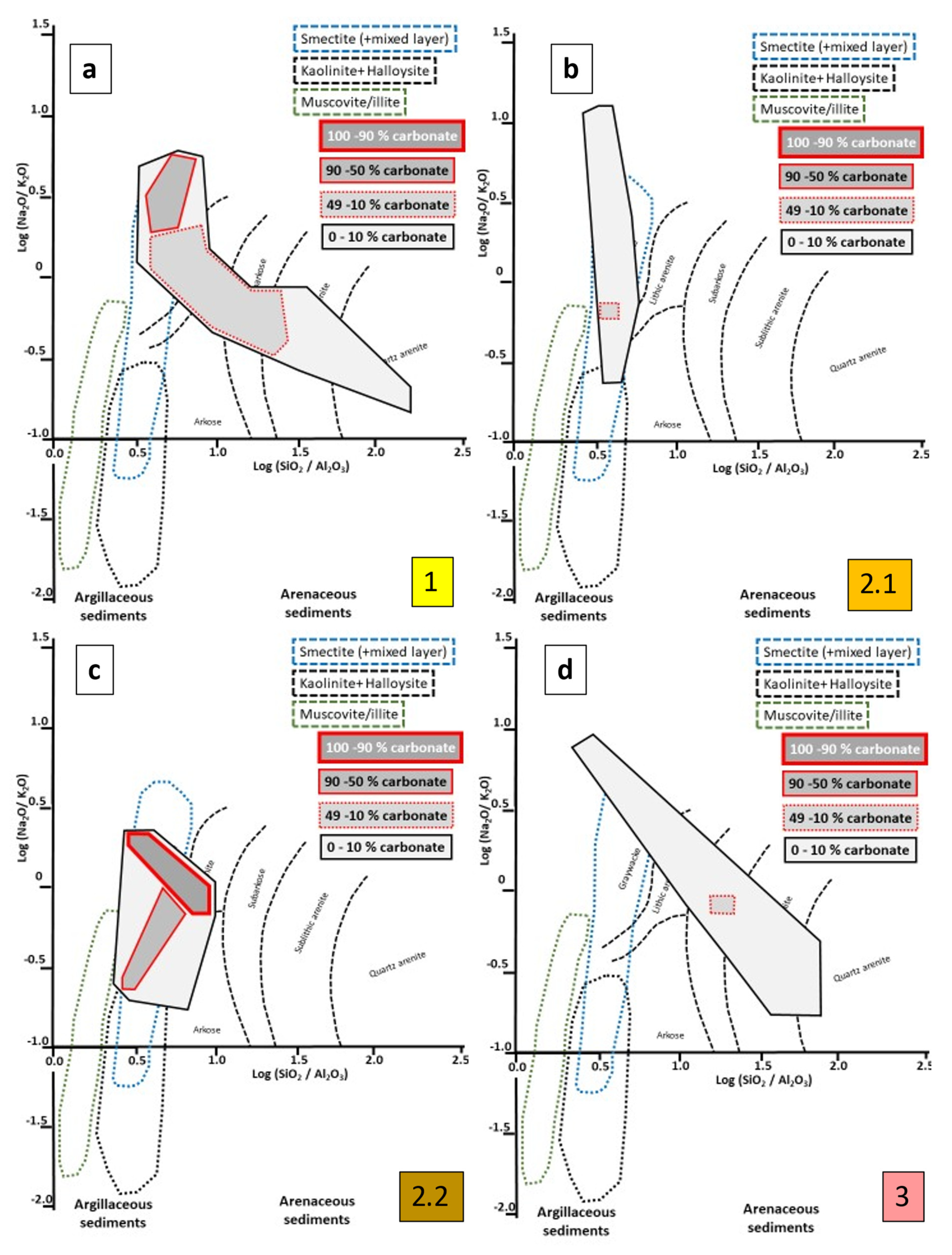
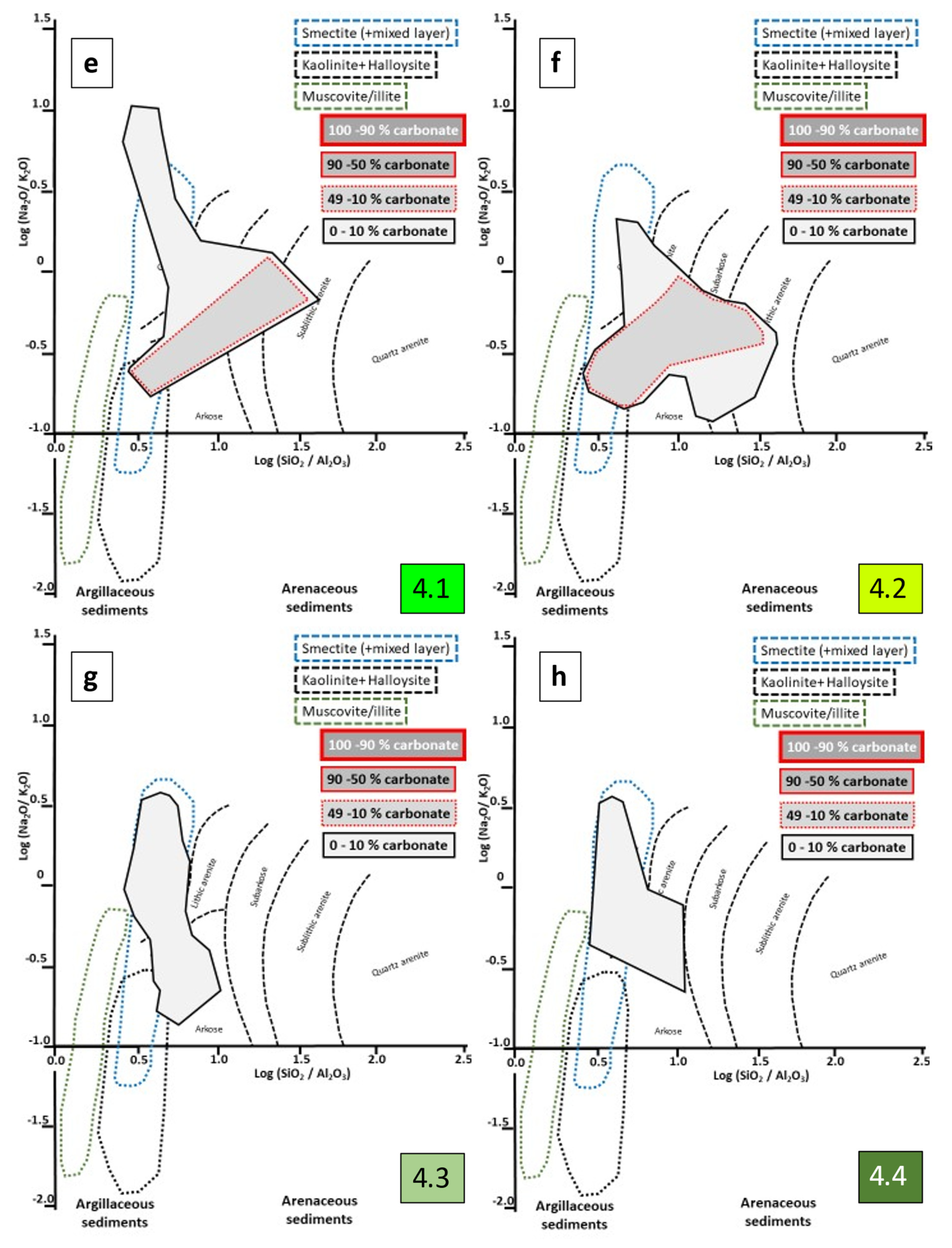
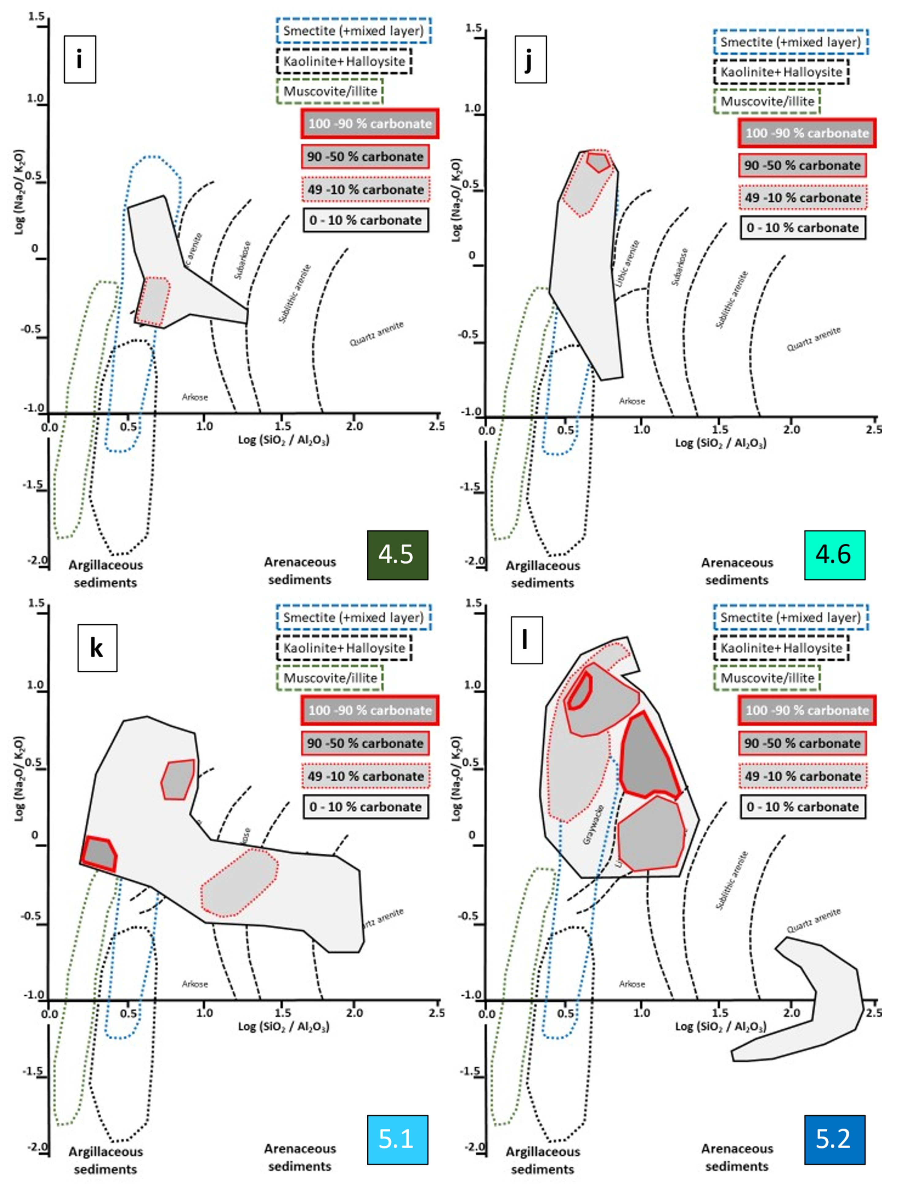
4.2.5. Calcareous and Non-Calcareous Argillaceous and Arenaceous Sediments and the Ratio log (SiO2/Al2O3) vs. log (Na2O/K2O)

The chemical composition of the sediments of the various LFS can be used as a supplementary tool to describe the depositional environment and to subdivide the siliciclastic sediments, as shown by the x-y plot of Pettijohn et al. [1] (1987), which forms the basis of Figure 14. Some amendments are made by the author with regard to the 7Å-(kaolinite-group), 10Å-(mica) and 14Å-(smectite group) clay minerals of argillaceous sediments and an overlay showing the carbonate content of the argillaceous and arenaceous sediments under study (Figure 1 and Figure 14o). In a direct comparison of the graphs, a strong tendency to mixed-type clastic sediments rather than pure quartz arenites is evident in these Quaternary sediments. Only in the aeolian LFS 1, the cryogenic LFS 3, and the marine LFS 5.1 and 5.2, can a small incursion into the quartz arenite territory be recognized (Figure 14a,d,k,l). Moreover, the element ratios of the various depositional environments can be subdivided into linear trends and clusters reflecting the strategy adopted for the aforementioned trend-line diagrams. Linear single-trend datasets can be seen for LFS 2.1 and LFS 3 (Figure 14b,d). Binary trends of datasets occur for LFS 1, 4.1, 4.2, 4.3, 4.4, 4.5 (?), 5.1 (?) and 6.3 (Figure 14a,e–i,k,n). Complex data arrays or unspecified data clusters are encountered for LFS 2.2, 5.2 and 6.1/6.2 (Figure 14c,i,m). The carbonate contents are another criterion useful for the fine-tuning of deposits and their distinction from each other, as demonstrated by the almost carbonate-free or carbonate-poor deposits, e.g., LFS 2.1 and 4.3, in contrast to carbonate-enriched environments, e.g., LFS 1, 5.2 and 6.3.

5. Discussion

5.1. Sedimentological Parameters vs. Composition—A Comparison

A homogeneous grain size distribution of unconsolidated clastic sediments may be the result of a long-distance transport, or a long-lasting and intensive transport with strong reworking. Particles very much different in their size may be due to a fast-motion landscape-forming process or they act as a proximity indicator in relation to the provenance area. Such observations can, locally, be made in the field with the naked eye or the hand-lens. For any comparison of sediments and a precise interpretation, however, these rather subjective observations are not sufficient and need follow-up laboratory analyses. The many sedimentary parameters have been given different names such as mean, median, sorting, skewness and kurtosis, which can be used in different ways [10,11,12,13,14,15,16]. The numerical data are good for a comparison of, e.g., bedforms, but they are not yet an expedient solution for a precise environment analysis. In addition to the grain size, this statement is also valid for the remaining two sedimentary parameters, grain shape and grain orientation [175,176,179]. The latter measurements only play a part when the grain size spectrum of the clastic sediments under consideration also covers gravel-sized grains, which is rarely the case in the current projects [75,180,181]. All sedimentological parameters are physical ones resulting from gravity-driven, aquatic and aeolian processes encompassing separation according to the specific gravity, grain morphology, bedform roughness and gradient.
Chemical facies analysis is a self-explanatory technical term and denotes the redox and the pH regimes, in addition to the wide range of solubles involved in the chemical processes under near-ambient conditions in the environment of the Quaternary deposits. The pioneering period of the classical chemical facies analysis was during the second half of the last century, but this analysis is still conducted today [182,183,184,185,186,187,188,189,190,191,192,193,194].
To obtain both physical and chemical parameters, a joint discussion of the two groups is a logical approach. This is a mirror image of what is known among sedimentologists as the textural and compositional maturity, which can be split into five classes: (1) immature, (2) submature, (3) low mature, (4) high mature, and (5) supermature [2]. While grain size decreases, the roundness, sphericity and sorting increase from the immature towards the supermature textural state (Table 5). The compositional maturity involves sediment load/density, the oxidation state and the carbonate content, which were computed from the diagrams and normalized to the maximum value of each column; this was set to 100 in this project on Quaternary sediments and mineral deposits (Figure 11, Figure 12, Figure 13 and Figure 14).
It has to be noted that, between the tripartite geomorphological-geodynamic maturity described previously in this review and the five-element sedimentological maturity subdivision discussed in this section, there are no qualitative but only hierarchical differences. The first is the 1st order subdivision considering the environment on a regional or continental scale, whereas the five-element sedimentological maturity classification is representative of the 2nd order level considering the environment on a local scale.

5.2. The Parametric Categorization of Landscape Forming Processes

5.2.1. Aeolian Processes

The landforms and the deposits of the LFS 1 develop after a long-distance dry unidirectional transport by wind [62,63,64] (Figure 4 and Figure 5). By analogy with the mud weight of a drilling operation, the air-dry transport operation under consideration is very light, indicated by the generally low HM content relative to the LM. Due to the long-distance transport, a good sorting coefficient can be expected (Figure 11a). The sphericity does not correspond to the amount of the major LM quartz and is the only parameter worsening the textural maturity. Multiple reworking with deflation and deposition areas adjacent to each other may cause an overprinting of LFS 4.1 and 4.5 deposits from braid plains or wadis where the particles are picked up. The peculiar fluvial environments leave their “fingerprint” on the aeolian sediments and dune fields, and thereby exert a controlling effect on the maturity index (Figure 12a–c). The overall highly oxidizing regimen under which dune fields normally develop can be deduced from the high Ti/Fe ratio (Figure 4 and Figure 13a) [36]. Active aeolian landforms laid bare come into existence under strongly oxidizing conditions, whereas fossiliferous, partially vegetated equivalent, landforms may even contain Fe disulfides indicative of a reducing regime. Chemical residues (e.g., carbocretes, sulcretes) are present in the fine-grained interdune sediments where they are diagnostic of more alkaline or acidic meteoric fluids. Clay minerals are present in coarser-grained fractions and more widespread in arid/semiarid and dry continental climate zones, which are the most active zones in terms of aeolian landforms. The aeolian landforms are abundant in carbonate and smectite-group clay minerals, which bear witness to an overall strongly alkaline meteoric fluid regime (Figure 14a and Table 5) [65,137].

5.2.2. Gravity-Driven Processes

Both land-forming processes coded LFS 2 and LFS 3 are discussed together because they are genetically closely related to each other, even if the climate zones where they predominantly operate are very different from each other [71,195]. They have been derived from fast short-distance to in situ processes under dry and wet conditions. They have a higher fluid density than the LFS 1, being in motion, but they display the same non-correlation between LM and sorting and, in places, develop under lower Eh values than LFS 1. The density mass wasting products are strongly influenced by the underlying bedrock and lithological well defined in contrast to the aeolian sediments that can pick up particles from different substrates and integrate them into a sand or dust storm. Not only does the specific gravity of the bedrock matter, but also the “lubricant”, which is frequently a mixture of water and finer-grained particles than coarse-grained material, and which is often mapped in the depocenter. Therefore, we have to differentiate between the stages of transport of mass wasting products which often result from polygenetic processes [196,197]. The latter is due to the processes which are periodic or episodic, and, when abandoned, allow vegetation to rapidly re-conquer and blanket these landforms with at least a pioneer soil and sparse vegetation (Figure 5). Much of that addressed for LFS 2 can also be applied to the landforms of LFS 3 [198,199]. The carbonate contents of LFS 2 strongly depend on the carbonate content of the bedrock and, to a lesser degree, on the carbocretes [161]. In the cryogenic LFS 3, H2O is present predominantly in the solid state as ice, so that chemical alteration based on highly mobile solubles is strongly impeded. Strikingly, the cryogenic LFS 3 contains the lowest carbonate content and its overlap with the stability field of the smectite group is small compared with LFS 2.1 and LFS 2.2. In terms of pH, the meteoric fluids of LFS 3 are rather acidic as witnessed by the lichens and mosses in the periglacial regions.

5.2.3. Confined and Unconfined Fluvially Driven Processes

The fluvial landform series LFS 4 is a fully aquatic pluri-directional long-distance land-forming process. From this brief and comprehensive description and its landforms depicted in Figure 7, it is clear that such a complex process cannot be attributed to one single textural maturity state and can hardly be squeezed into a single environmental compartment [24,25,26,27,28,29,30,31,32,33] (Table 5). It is feasible to determine the sediment load, density and alkalinity of the various drainage systems and their perennial or ephemeral water floods [200,201]. The redox conditions of the active fluvial drainage system developed under oxidizing conditions. Reducing conditions occur at the edge of abandoned fluvial drainage systems where oxbow and cut lakes form in a similar manner to that of perennial lakes regarding the sedimentology and sediment chemistry (Table 4 and Table 5) [145,146,202,203]. Precise markers of shallow ground water levels, which are quite common to fluvial flood plains, are found within the realm of soil types. Some of these, indicative of stagnant poorly aerated water regimes, are displayed in Figure 9.
The tide-dominated estuaries and the wave- and fluvial-dominated deltas (LFS 4.6) terminate the river run before entering the final marine or lacustrine depocenter (LFS 6.1). They fulfill all criteria (see above) for a high degree of textural maturity, whereas braided (LFS 4.1), straight (LFS 4.3) and ephemeral streams (LFS 4.5) are proximal to the source (headwaters) or only intermittently carry water, qualifying them for a low mature to submature stage (Table 5). From the compositional perspective, LFS 4.4 stands out with regard to its “sediment-load density”. There are flood hazards characterized by a “slurry” overloaded with debris that spreads across plains in the form of flash floods or sheetfloods. The reasons for such hazards are manifold and range from ice jam flooding to downpours in the desert that occur only periodically or episodically. The transition from unconfined LFS 4.4 into confined drainage systems of LFS 4.3 and LFS 4.5 is gradual and accompanied by what might be illustrated by technical processes and expressed again in terms of drill-mud engineering as a lowering of the “mud weight” (Table 5 and Figure 7a,d,l,m) [99,100,148,204,205,206,207]. These LFSs are characterized by an oxidizing regime, whereas the carbonate content and the pH of the meteoric fluids changes according to the degree of evaporation and results in the duricrusts depicted in Table 5 and Figure 9n–q. The wadis of LFS 4.5 are more prone to calcretes than the gullies of LFS 4.3 (Figure 7d,I). The meandering or high-sinuosity streams are abundant in the regions investigated throughout this project and take an intermediate position regarding the compositional and textural maturity (Table 5 and Figure 7h,i).

5.2.4. Coastal-Marine Processes

LFSs 5.1 and 5.2 are both restricted to a rather narrow “semi-aquatic” strip of landscape between land and sea called the coastal zone [117]. The shallow water actions and the effect of waves are manifold and denominated as refraction, breaking, erosion, etc., and are directed more or less perpendicular to the shoreline. Depending on the tidal-range, the back-and-forth is stronger in LFS 5.1 than in LFS 5.2, a fact that is also inherent to the process-related subdivision of the environment into macro- and microtidal regimes (Figure 8). In this LFS, the carbonate content, which normally is held to be a marker of the pH value of the meteoric fluids, is cast in the role of a measure of the amount of calcareous bioclasts. One of the most frequent sub-environments in the wave-dominated LFS 5.2 is the reefal environment, with landforms created by, e.g., coral reef builders under the water and brought into the reaches of the waves as the sea level drops and unconsolidated bioclastic rubble is piled on the beach around the reef edifice or scattered across flattened keys (Figure 8j,k) [132,208,209,210]. This difference is also conspicuously reflected by the degree of textural maturity and the density of the sediment load (Table 5). The vast intertidal flats and supratidal landward zones of the tide-dominated coasts are permanently or periodically exposed, so as to render them amenable to sampling the data, of which the redox marker is useful and accounts for the higher degree of oxidation (Table 5 and Figure 8a–f) [129].

5.2.5. Lacustrine Processes

LFS 6.2 is representative of a continental stagnant water body placed at the end of a clastic transport route along which prevalently fluvial (LFS 5) and mass wasting (LFS 4) processes shaped the mineral matter in terms of a decrease in size and an improvement of sphericity and grain morphology (Table 5). Not surprisingly, the textural maturity achieves its maximum in the perennial LFS 6.2, whereas the sediment load decreases to a relative minimum after passing through the marginal facies zone of the lake [20]. LFS 6.1 encompasses, among other types, meander, oxbow and levee lakes, bridging the gap to LFS 4.2 (Figure 7h). The characteristic features of LFS 6.1 are akin to those of LFS 4.2, connecting the anabranching and deltaic channel types to the true lacustrine environment of LFS 6.2 (Table 5). The different trend can be observed in the ephemeral lakes of LFS 6.3, where duricrusts, mainly enriched in carbonate, sulfate and chloride, are concentrated by strong evaporation on a periodic or episodic basis in a fine-grained siliciclastic matrix [136,202,211] (Figure 9n,o).

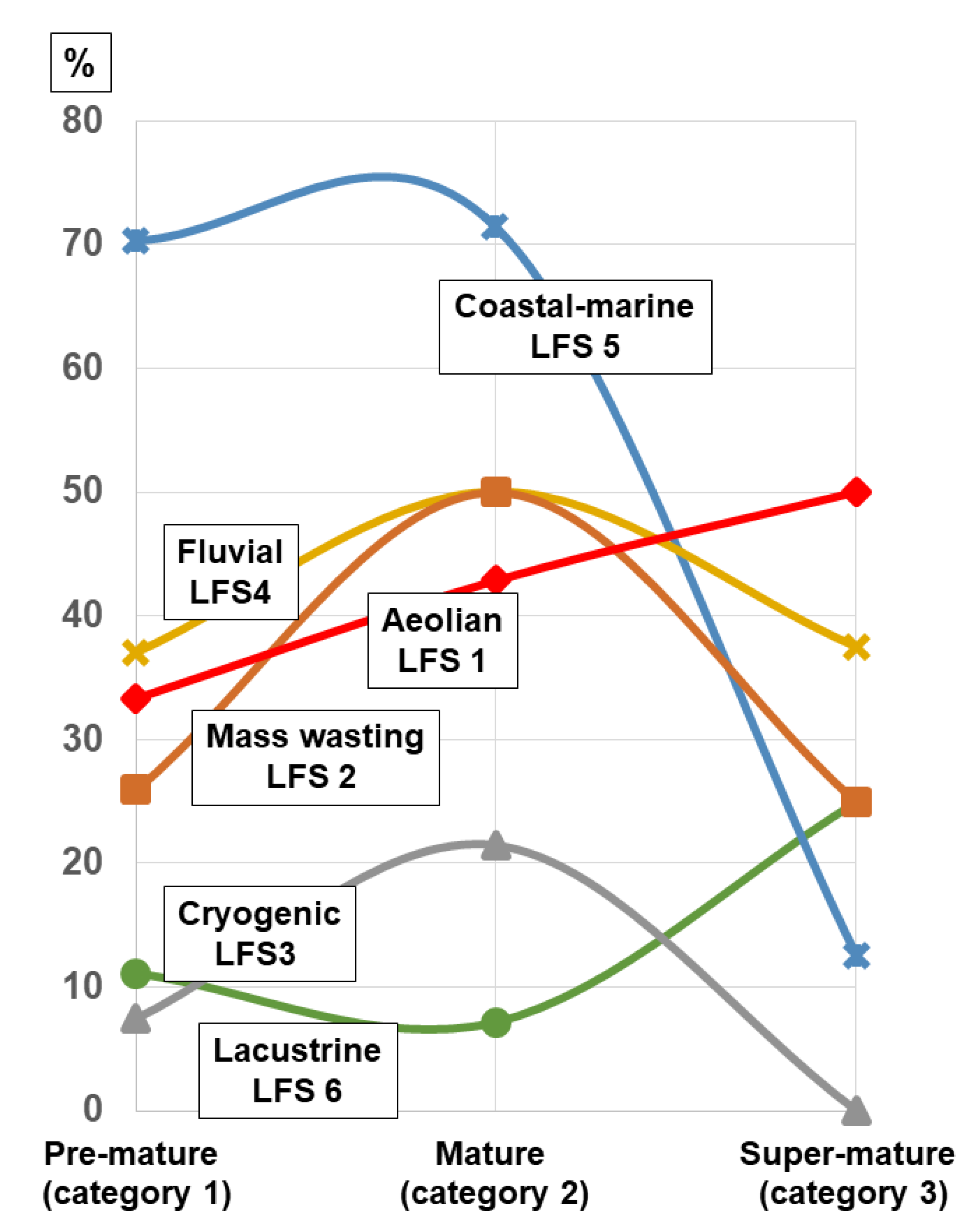
5.3. Geomorphological-Geodynamic Maturity vs. Environment of Deposition

In the tripartite geomorphological-geodynamic maturity classification, the intermediate category 2 takes the top position on the scale of the land-forming intensity, highlighted by the maxima of fluvial, cryogenic, mass wasting and coastal-marine processes (Figure 15). In general, this crustal section provides a good blend, combining both aspects of planation during deformational quiescence, and considerable tectonic activity that is held to be accountable for the incision of valleys [56,58,98,212,213,214] (Figure 15).
The Caledonian, Variscan and Cimmerian orogenies representative of category 2 operated during the Paleozoic and Mesozoic and resulted in the preservation of remnants of pene-plained landscapes, whereas the Alpine and Andean orogenies were only looming and at an early deformational stage [54,55,56,57]. The latter worldwide orogenies experienced their climax state during the Cenozoic era when they became the reference type of mature category 1. This temporal relationship of the three Paleozoic-Mesozoic orogenies predominantly fosters slope- and gradient-related land-forming processes such as fluvial and mass-wasting processes. Even if the current overview study is not designed to constitute a quantitative picture of the Earth’s surface in terms of crustal maturity in the context of their physical and chemical parameters, this concept reflects the linkages of geodynamic and geomorphological processes as a function of the crustal maturity, and can cater to the needs and wants of genetic and applied geosciences on a regional and local scale; see also Section 5.5 (Figure 3 and Figure 15). In general, the pre-mature category 1 does not include of the six processes to form a maximum in its bounds, even if it undoubtedly shows an eye-catching and picturesque panorama [215]. It is a crustal section with significant geodynamic rises and falls, also mirrored by the variegated landforms remaining in what might be called a “metastable state”. This scenario is totally different from the super-mature category 3, which breaks some “negative” (LFS 3, 5) and “positive” (LFS 1, 6) records in terms of the intensity of land-forming processes (Figure 15). Land-forming processes that are unrelated to strong gradients but in need of vast inland plains to reach full maturity, such as the aeolian and the lacustrine processes, find perfect prerequisites in the deeply eroded crustal sections resting in relative deformational quiescence. Unimpeded by any natural obstacles, wind action can exert its full strength and give rise to the aeolian sand seas, e.g., Simpson Desert and Great Sandy Desert Australia; Kalahari and Namib Deserts, southern Africa; Rub al Khali, Arabian Peninsula [65,216]. This is also true for the ephemeral lakes, which spread across the continental interiors [138,217]. The latter environments also provide ideal deflation pans and source areas for the fine-grained particles of the dunes of LFS 1. The low-latitude position of these geodynamic zones proximal to the equator in the Northern and Southern Hemispheres provides a further boost to these LFS 1 landforms due to the high rate of evaporation under tropical arid climates. The mature category 3 also stands out due to a marked minimum regarding the cryogenic landforms, which is self-explanatory in view of the climate zonation relative to the latitudinal position (Figure 1 and Figure 3). The same is true for the coastal-marine processes (LFS 5). The Precambrian cratons form the nuclei of the modern-day continents in Africa and the Americas, and are mostly covered and rimmed by younger platform sediments reaching the coastal zones [218]. Regarding the marine LFS, the geodynamically related lithological and structural features of the Precambrian rocks can only take immediate effect in a few places along the coastal zones of the continents, such as on both sides of the Red Sea, along the SW African coast, or on the Brazilian Coast [45].

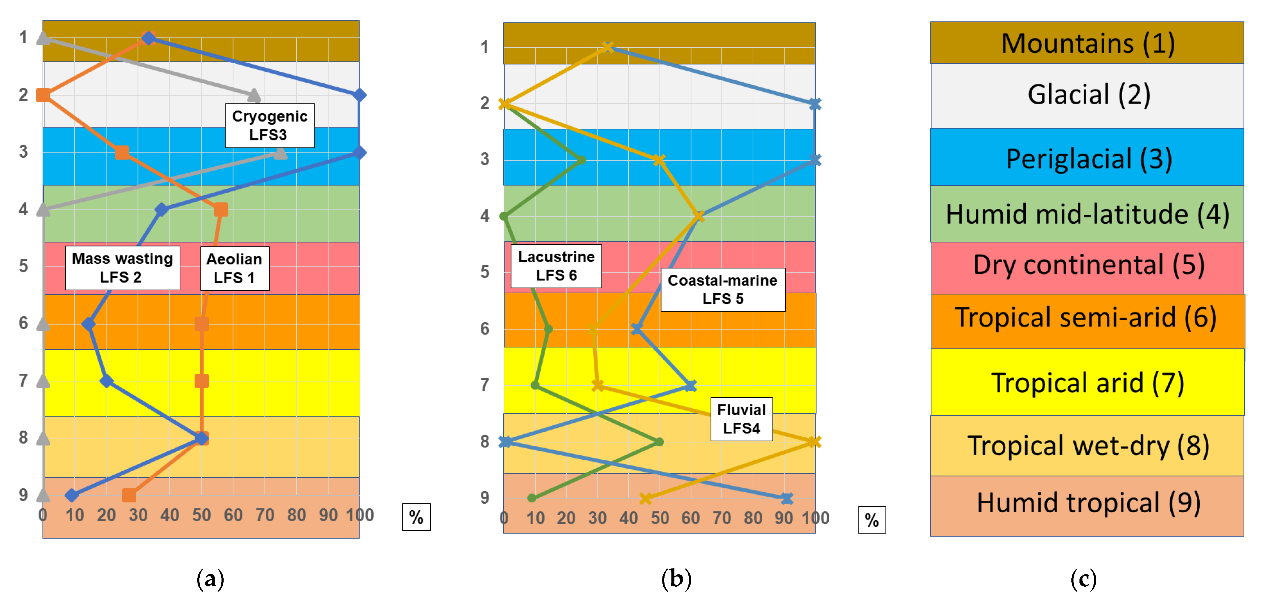
5.4. Climate vs. Environment of Deposition

Some graphs similar to that used during the geomorphological-geological maturity discussion were drafted for the LFSs under study to show their positioning as a function of the climate zonation and, hence, facilitate the discussion of the climate impact on the previous diagrams (Figure 15 and Figure 16). A relative maximum is found for the mass wasting and cryogenic processes in the glacial and periglacial climate zones where mechanical/physical weathering prevails over chemical weathering (Figure 16a). The joint operation of true glacial processes resulting in different types of moraines and subglacial landforms and fast-moving mass wasting processes, such as landslides and catastrophic debris flows, shaped the valleys that were cut into the crust during the period from the Last Glacial Maximum to the Holocene [40,89,219,220] (Figure 6). Mass wasting activity in the study areas reaches a low from the humid-mid-latitude to the tropical wet-and-dry climates (Figure 5 and Figure 16a). The frequency and intensity of extreme weather events triggered the fast-moving mass wasting processes in the tropical semiarid and arid climate zones [221,222,223,224]. These spot-like land-forming processes are responsible for the minimum in the graph of Figure 16a. In contrast to LFS 1 and LFS 2, LFS 3 displays a constantly low level of intensity from the humid mid-latitude to the tropical dry-and-wet climate zone due to the high temperature. The course of the graph in Figure 16a is a small-scale textbook example of aeolian transport and deposition [66] (Figure 4). Deposition of sand and the emplacement of aeolian landforms is stimulated by wetness, surface roughness and natural obstacles resulting from vertical tectonic movements, which may reduce the windspeed to the level at which saltation and suspension of particles is no longer feasible. The wetter climate zone towards the pole and the equator are more favorable for vast blankets, or at least a patchy vegetation, so that dunes may still exist there. However, many of these are abandoned today and date back to a climate that was more “aeolian-friendly” than during the recent climate zones (cold dry continental) (Figure 1). It is a marker of the climate change during the recent history of the Earth [225,226,227] (Figure 16a).
Table 3 and Table 4 and more proximal to the equator by the passage from climate zone 7 into climate zone 8 (Figure 16b,c) [228,229,230,231,232]. The graph of the fluvial processes is paralleled by the lacustrine graph, which indicates the extension and shrinking of perennial lakes along with these climate changes and variable vegetation in its immediate surroundings, consistent with these atmospheric processes [204]. The climate-related coastal-marine trend is decoupled from those of the remaining land-forming processes, excluding the cryogenic and mass wasting processes (Figure 16b). The shoreline or cliff retreat as a consequence of sea level rise is accompanied by slow- or fast-moving mass wasting processes or freeze–thaw cycles [233]. Fluvial, particularly fluvial deltaic, subtypes provoked an opposite trend in the back-and-forth motion of coastal zones.

5.5. Synopsis—The Present Is the Key to the Past vs. from Review to Manual

The joint sedimentological-chemical-mineralogical investigation of the depositional environments of unconsolidated Quaternary clastic sediments is not treated as an end in itself. This investigation is a logical and supporting measure to cater for the needs and wants of the E & E issue (economic geology and environmental geology) in applied geosciences, as their intrinsic methods are no longer able to offer unequivocal results and help address the related problems [37,107]. As such, it discards any idea of claiming to cover the entire surface of the globe, which would be a Herculean task for anyone. The investigation developed in the course of studying and exploring sedimentary or sediment-hosted pre-Quaternary mineral deposits from aluminum to zirconium, which were emplaced by processes from the fluvial incision and slope retreat by mass wasting, to the clastic deposits of lakes and reefal islands or cays fringing the coastal zone towards the open sea [37,234,235,236,237,238]. It was designed to better understand the evolution of mineral deposits and their environment of formation. With the latter aspect in mind, it will also be of aid for the fields of environmental geology, engineering geology and urban geology, which aim to identify waste disposal areas or to delineate those areas susceptible to inundation or jeopardized by general natural hazards, or, in general, where the anthropogenic impact encounters nature. Because the current review transforms into a kind of manual, it does not reflect a final state of evolution, but is open to amendments according to the issues faced by a potential user.
It has to be noted that none of the trend lines indicative of the “typical rainy cloud patterns”, with a sharp upper limit on the y-axis and a more or less wide spread along the x-axis, or the compositional x-y plots, should be used as a stand-alone tool. They can only be used effectively in combination and, if necessary, should be supplemented by, e.g., age dating or other advanced geoscientific analytical methods. For the radio-carbon dating of Quaternary sediments, optical stimulated luminescence, K/Ar and Ar-Ar, and U/Pb and U-Th dating have proved to provide additional valuable chronological data for the environments. Conversely, the use of advanced analytical methods or age dating without the application of the basic methods on display in the flow chart of Figure 2 may yield datasets.

6. Conclusions

  • A joint sedimentological-chemical-mineralogical investigation of the depositional environment of unconsolidated clastic sediments of the Quaternary forms both the nucleus of a series of global reference sites and a manual to preferentially guide the audience from applied geosciences about how to make further amendments to individual projects of economic and environmental geology (i.e., the E & E issue).
  • Trend diagrams and compositional x-y plots can contribute to constraining the development of the entire set of landform series built-up by clastic sedimentary deposits.
  • Taking the current joint approach, the full transect, from the fluvial incision and slope retreat high in the mountains, to the reef islands fringing the coastal zone towards the open sea, can be taken as a reference. This joint approach bridges the gap between a true review based only on the existing literature and a hybrid manual based on data gathered from practical field studies in applied geosciences, known as extractive and environmental geology (i.e., the E & E issue, a term coined by the author).
  • Climate zonation and crustal maturity directly impact the datasets and, consequently, both exogenous and endogenous “drivers” can be deduced from the compositional (mineralogy and chemistry) and physical (transport and deposition) variations observed in the Quaternary sediments, illustrated by trend and x-y plots, and also applied to the pre-Quaternary target areas.
  • Environment analysis, whether an end in itself or used as a supplement to economic/extractive geology and/or anthropogenic and engineering geology, is too complex to allow assumptions and models to be based on the use of stand-alone graphs. It is, however, the only means to create a sound platform for the discussion and application of advanced investigations during a terrain analysis (2-D) or basin analysis (3-D), according to the elaborated flow chart.

Funding

This research received no external funding.

Institutional Review Board Statement

Not applicable.

Informed Consent Statement

Not applicable.

Data Availability Statement

Not applicable.

Acknowledgments

I acknowledge with thanks the critical comments made by two anonymous reviewers regarding the original version of this invited Feature Paper. I also extend my gratitude to the acting editor, Phattranit Sophon.

Conflicts of Interest

The author declares no conflict of interest.

References

  1. Pettijohn, F.J.; Potter, P.E.; Siever, R. Sand and Sandstone; Springer: Berlin/Heidelberg, Germany, 1987; 553p. [Google Scholar]
  2. Friedman, G.M.; Sanders, J.E.; Kopaska-Merkel, D.C. Principles of Sedimentary Deposits; MacMillan Publishing Company: New York, NY, USA, 1992; 717p. [Google Scholar]
  3. Wilson, M.A. Macroborings and the evolution of bioerosion. In Trace Fossils: Concepts, Problems, Prospects; Miller, W., III, Ed.; Elsevier: Amsterdam, The Netherlands, 2007; pp. 356–367. [Google Scholar]
  4. Jensen, S. Paleontology: Reading Behavior from the Rocks. Science 2008, 322, 1051–1052. [Google Scholar] [CrossRef]
  5. MacEachern, J.; Pemberon, S.G.; Gingras, M.K.; Bann, K.L. Ichnology and Facies Models. In Facies Models 4; James, N., Dalrymple, R.W., Eds.; Geological Association of Canada: St. John’s, NL, Canada, 2010; pp. 19–58. [Google Scholar]
  6. Reineck, H.E.; Singh, I.B. Depositional Sedimentary Environments: With Reference to Terrigenous Clastics; Springer Science Business Media: New York, NY, USA, 2012; 551p. [Google Scholar]
  7. Prothero, D.R.; Schwab, F. Sedimentary Geology, 3rd ed.; W.H. Freeman: New York, NY, USA, 2014; 500p. [Google Scholar]
  8. Udden, J.A. Mechanical composition of clastic sediments. Geol. Soc. Am. Bull. 1914, 25, 655–744. [Google Scholar] [CrossRef]
  9. Wentworth, C.K. A Scale of Grade and Class Terms for Clastic Sediments. J. Geol. 1922, 30, 377–392. [Google Scholar] [CrossRef]
  10. Krumbein, W.C. The probable error of sampling sediments for mechanical analysis. Am. J. Sci. 1934, 27, 204–214. [Google Scholar] [CrossRef]
  11. Inman, D.L. Measures for describing the size distribution of sediments. J. Sed. Petr. 1952, 22, 125–145. [Google Scholar]
  12. Folk, R.L.; Ward, W.C. Brazos River bar: A study in the significance of grain size Parameters. J. Sed. Petr. 1958, 27, 3–26. [Google Scholar] [CrossRef]
  13. McCommon, R.B. Efficiencies of percentile measures for describing the mean size and sorting of sedimentary particles. J. Geol. 1962, 70, 453–465. [Google Scholar] [CrossRef]
  14. Passega, R.; Byramjee, R. Grain-size image of clastic deposits. Sedimentology 1969, 13, 233–252. [Google Scholar] [CrossRef]
  15. Visher, G.S. Grain-size distributions and depositional processes. J. Sediment. Petrol. 1969, 39, 1074–1106. [Google Scholar]
  16. Tucker, M.E. Sedimentary Rocks in the Field; John Wiley & Sons: Chichester, UK, 1996; 153p. [Google Scholar]
  17. Bari, Z.; Rajib, M.; Majid, M.; Sayem, H. Textural analyses of the bar sands of the Gorai River: Implications for depositional phase and environment. Jahangirnagar Univ. Environ. Bull. 2012, 1, 25–34. [Google Scholar] [CrossRef] [Green Version]
  18. Liro, M. Differences in the reconstructions of the depositional environment of overbank sediments performed using the C/M diagram and cumulative curve analyses. Landf. Anal. 2015, 29, 35–40. [Google Scholar] [CrossRef]
  19. Ma, L.; Wu, J.; Abuduwaili, J. Variation in Aeolian Environments Recorded by the Particle Size Distribution of Lacustrine Sediments in Ebinur Lake, Northwest China; Springer: Berlin/Heidelberg, Germany, 2016; p. 481. [Google Scholar] [CrossRef] [Green Version]
  20. Warrier, A.K.; Pednekar, H.; Mahesh, B.S.; Mohan, R.; Gazi, S. Sediment grain size and surface textural observations of quartz grains in late Quaternary lacustrine sediments from Schirmacher Oasis, East Antarctica: Paleoenvironmental significance. Polar Sci. 2016, 10, 89–100. [Google Scholar] [CrossRef]
  21. Wu, X.; Liu, G.; Ji, S. Grain size variation and its environmental significance from Huguangyan Maar Lake, Zhanjiang since the Holocene. J. Lake Sci. 2016, 28, 1115–1122. [Google Scholar]
  22. Baiyegunhi, C.; Liu, K.; Gwavava, O. Grain size statistics and depositional pattern of the Ecca Group sandstones, Karoo Supergroup in the Eastern Cape Province, South Africa. Open Geosci. 2017, 9, 554–576. [Google Scholar] [CrossRef]
  23. Kong, H.; Wang, L.; Zhang, H. The variation of grain size distribution in rock granular material in seepage process considering the mechanical–hydrological–chemical coupling effect: Experimental research. R. Soc. Open Sci. 2020, 7, 190590. [Google Scholar] [CrossRef] [Green Version]
  24. Williams, G.P. River meanders and channel size. J. Hydrol. 1986, 88, 147–164. [Google Scholar] [CrossRef]
  25. Miall, A.D. The Geology of Fluvial Deposits; Springer: New York, NY, USA, 1996; 582p. [Google Scholar]
  26. Knighton, D.A. Fluvial Forms and Processes: New Perspective; Arnold: London, UK, 1998; 400p. [Google Scholar]
  27. Nanson, G.C.; Knighton, A.D. Anabranching rivers: Their cause, character and classification. Earth Surf. Processes Landf. 1996, 21, 217–239. [Google Scholar] [CrossRef]
  28. Selley, R.C. Applied Sedimentology, 2nd ed.; Academic Press: Cambridge, MA, USA, 2000; 523p. [Google Scholar]
  29. Chin, A. The periodic nature of step-pool mountain streams. Am. J. Sci. 2002, 302, 144–167. [Google Scholar] [CrossRef] [Green Version]
  30. Moody, J.A.; Troutman, B.M. Characterization of the spatial variability of channel morphology. Earth Surf. Processes Landf. 2002, 27, 1251–1266. [Google Scholar] [CrossRef]
  31. Bridge, J.S. Rivers and Floodplains; Whiley-Blackwell: Oxford, UK, 2003; 504p. [Google Scholar]
  32. Robert, A. River Processes: An Introduction to Fluvial Dynamics; Routledge: Abingdon, UK, 2003; 238p. [Google Scholar]
  33. Charlton, R. Fundamentals of Fluvial Geomorphology; Routledge: Abingdon, UK, 2014; 214p. [Google Scholar]
  34. Tricart, J.; Cailleux, A. Introduction to Climatic Geomorphology; Longman: London, UK, 1972; 295p. [Google Scholar]
  35. Scotese, C.R. Paleomap Project. 2002. Available online: http://www.scotese.com/legend.htm (accessed on 26 October 2021).
  36. Dill, H.G. Residual clay deposits on basement rocks: The impact of climate and the geological setting on supergene argillitization in the Bohemian Massif (Central Europe) and across the globe. Earth Sci. Rev. 2017, 165, 1–58. [Google Scholar] [CrossRef]
  37. Dill, H.G. The “chessboard” classification scheme of mineral deposits: Mineralogy and geology from aluminum to zirconium. Earth Sci. Rev. 2010, 100, 1–420. [Google Scholar] [CrossRef]
  38. Dill, H.G. A geological and mineralogical review of clay mineral deposits and phyllosilicate ore guides in Central Europe—A function of geodynamics and climate change. Ore Geol. Rev. 2020, 119, 103304. [Google Scholar] [CrossRef]
  39. Dill, H.G.; Kaufhold, S.; Techmer, A.; Baritz, R.; Moussadek, R. A joint study in geomorphology, pedology and sedimentology of a Mesoeuropean landscape in the Meseta and Atlas Foreland (NW Morocco). A function of parent lithology, geodynamics and climate. J. Afr. Earth Sci. 2019, 158, 103531. [Google Scholar] [CrossRef]
  40. Dill, H.G.; Buzatu, A.; Goldmann, S.; Kaufhold, S.; Bîrgăoanu, D. Coastal landforms of “Meso-Afro-American” and “Neo-American” landscapes in the periglacial South Atlantic Ocean: With special reference to the clast orientation, morphology, and granulometry of continental and marine sediments. J. S. Am. Earth Sci. 2020, 98, 102385. [Google Scholar] [CrossRef]
  41. Dill, H.G.; Buzatu, A.; Balaban, S.-I.; Ufer, K.; Gómez Tapias, J.; Bîrgăoanu, D.; Cramer, T. The “badland trilogy” of the Desierto de la Tatacoa, Upper Magdalena Valley, Colombia, a result of geodynamics and climate: With a review of badland landscapes. Catena 2020, 194, 104696. [Google Scholar] [CrossRef]
  42. Gordon, B.L. In Defense of Uniformitarianism. Perspect. Sci. Christ. Faith 2013, 65, 79–86. [Google Scholar]
  43. Dill, H.G.; Buzatu, A.; Balaban, S.-I. Coastal morphology and heavy mineral accumulation in an upper-macrotidal environment—A geological-mineralogical approach from source to trap site in a natural placer laboratory (Channel Islands, Great Britain). Ore Geol. Rev. 2021, 138, 104311. [Google Scholar] [CrossRef]
  44. Summerfield, M.A. Global Geomorphology; John Wiley & Sons Inc.: New York, NY, USA, 1991; 537p. [Google Scholar]
  45. Russian Academy of Sciences Institute of Geography. Resources and Environment. In World Atlas I and II—Wien; Austrian Institute of East and Southeast European Studies: Hölzel, Vienna, 1998. [Google Scholar]
  46. Kottek, M.; Grieser, J.; Beck, C.; Rudolf, B.; Rubel, F. World Map of the Köppen–Geiger climate classification updated. Meteorol. Z. 2006, 15, 259–263. [Google Scholar] [CrossRef]
  47. Gómez, J.; Montes, N.E.; Nivia, Á.; Diederix, H. Geological Map of Colombia 2015. Scale 1:1,000.000; Servicio Geológico Colombiano: Bogotá, Colombia, 2015.
  48. Buchely, F.; Gómez, L.; Buitrago, J.; Cristancho, A.; Moreno, M.; Romero, O.; Hincapié, G.; Castro, F.; Ramos, J.; Casas, R.; et al. Geología de la Plancha 324 Tello Escala 1:100.000; Memoria Explicativa, INGEOMINAS; Colombian Geological Survey: Bogotá, Colombia, 2015; 152p.
  49. Steck, A.; Spring, L.; Vannay, J.-C.; Masson, H.; Stutz, E.; Bucher, H.; Marchant, R.; Tièche, J.C. Geological transect across the Northwestern Himalaya in eastern Ladakh and Lahul (A Model for the continental collision of India and Asia). Eclogae Geol. Helv. 1993, 86, 219–263. [Google Scholar]
  50. Yin, A. Cenozoic tectonic evolution of the Himalayan orogen as constrained by along-strike variation of structural geometry, exhumation history, and foreland sedimentation. Earth-Sci. Rev. 2006, 76, 1–13. [Google Scholar] [CrossRef]
  51. Greenway, M.E. The Geology of the Falkland Islands; Scientific Report; British Antarctic Survey: London, UK, 1972; Volume 76, pp. 1–42. [Google Scholar]
  52. Stone, P. The Geology of the Falkland Islands. NERC Open Research Archive, 2010. Available online: nora.nerc.ac.uk/10862/1/DepositsArticle-FI.pdf (accessed on 26 October 2021).
  53. Cocks, L.R.M.; Torsvik, T.H. European geography in a global context from the Vendean to the end of the Paleozoic. In European Lithosphere Dynamics, Geological Society of London Memoirs; Gee, D.G., Stephenson, R.A., Eds.; The Geological Society: Bath, UK, 2006; Volume 32, pp. 83–95. [Google Scholar]
  54. Elvevold, S.; Dallmann, W.; Blomeier, D. Geology of Svalbard; Norwegian Polar Institute/Norsk Polarinstitutt: Tromsø, Norway, 2007; 36p. [Google Scholar]
  55. Matte, P. The Variscan collage and orogeny (480 ± 290 Ma) and the tectonic definition of the Armorica microplate: A review. Terra Nova 2001, 13, 122–128. [Google Scholar] [CrossRef]
  56. McCann, T. The Geology of Central Europe: Precambrian and Palaeozoic: 1; Special Volume; The Geological Society of London: London, UK, 2008; 748p. [Google Scholar]
  57. Golonka, J.; Embry, A.; Krobicki, M. Late Triassic Global Plate Tectonics. In The Late Triassic World. Topics in Geobiology 46; Tanner, L., Ed.; Springer International: Berlin/Heidelberg, Germany, 2018. [Google Scholar] [CrossRef]
  58. McCann, T. The Geology of Central Europe: Mesozoic and Cenozoic: 2; Special Volume; The Geological Society of London: London, UK, 2008; 700p. [Google Scholar]
  59. Gutiérrez, M.; Gutiérrez, F. Climatic Geomorphology. Treatise Geomorphol. 2013, 13, 115–131. [Google Scholar]
  60. Dèzes, P.; Schmid, S.M.; Ziegler, P.A. Evolution of the European Cenozoic Rift System: Interaction of the Alpine and Pyrenean orogens with their foreland lithosphere. Tectonophysics 2004, 389, 1–33. [Google Scholar] [CrossRef]
  61. Peel, M.C.; Finlayson, B.L.; McMahon, T.A. Updated world map of the Köppen–Geiger climate classification. Hydrol. Earth Syst. Sci. 2007, 11, 1633–1644. [Google Scholar] [CrossRef] [Green Version]
  62. Muhs, D.R. Loess deposits, origins and properties. In Encyclopedia of Quaternary Science; Elias, S.A., Ed.; Elsevier: Amsterdam, The Nerherland, 2007; pp. 1405–1418. [Google Scholar]
  63. Lancaster, N. Dune Dynamics and Morphology. In Arid Zone Geomorphology; Thomas, A.S.G., Ed.; Wiley-Blackwell: Hoboken, NJ, USA, 2011; pp. 487–516. [Google Scholar]
  64. Mountney, N.P. A stratigraphic model to account for complexity in aeolian dune and interdune successions. Sedimentology 2012, 59, 964–989. [Google Scholar] [CrossRef]
  65. Rodriguez-Lopez, J.P.; Clemmensen, L.B.; Lancaster, N.; Mountney, N.P.; Veiga, G.D. Archean to Recent aeolian sand systems and their sedimentary record: Current understanding and future prospects. Sedimentology 2014, 61, 1487–1534. [Google Scholar] [CrossRef]
  66. Dill, H.G.; Buzatu, A. From the aeolian landform to the aeolian mineral deposit in the present and its use as an ore guide in the past. Constraints from mineralogy, chemistry and sediment petrography. Ore Geol. Rev. 2021, 104490. [Google Scholar] [CrossRef]
  67. Bastian, L.V. Residual soil mineralogy and dune subdivision, Swan Coastal Plain, Western Australia. Aust. J. Earth Sci. 1996, 43, 31–44. [Google Scholar] [CrossRef]
  68. Newsome, D. Origin of sandplains in Western Australia: A review of the debate and some recent findings. Aust. J. Earth Sci. 2000, 47, 695–706. [Google Scholar] [CrossRef]
  69. Andreucci, S.; Clemmensen, L.B.; Pascucci, V. Transgressive dune formation along a cliffed coast at 75 ka in Sardinia, Western Mediterranean: A record of sea level fall and increased windiness. Terra Nova 2010, 22, 424–433. [Google Scholar] [CrossRef]
  70. Noppradit, P.; Schmidt, C.; Dürrast, H.; Zöller, L. Late Quaternary evolution of Songkhla Coast, Southern Thailand, revealed by OSL Dating. Chiang Mai J. Sci. 2019, 46, 152–164. [Google Scholar]
  71. Schuster, R.L.; Highland, L.M. Overview of the Effects of Mass Wasting on the Natural Environment. Environ. Eng. Geosci. 2007, 13, 25–44. [Google Scholar] [CrossRef]
  72. Boelhouwers, J. Relict periglacial slope deposits in the Hex River Mountains, South Africa: Observations and Palaeoenvironmental Implications. Geomorphology 1999, 30, 245–258. [Google Scholar] [CrossRef]
  73. Paasche, Ø.; Strømsøe, J.R.; Dahl, S.E.; Linge, H. Weathering characteristics of arctic islands in northern Norway. Geomorphology 2006, 82, 430–452. [Google Scholar] [CrossRef]
  74. Hartvich, F.; Vilímek, V. Selected landforms and their significance in the analysis of the slope origin in the Losenice river valley, Šumava Mts. Acta Geodyn. Geomater 2008, 151, 275–296. [Google Scholar]
  75. Nieuwenhuijzen, M.E.; Van Steijn, H. Alpine debris flows and their sedimentary properties. A case study from the French Alps. Permafr. Periglac. Process. 1990, 1, 111–128. [Google Scholar] [CrossRef]
  76. Stock, J.D.; Montgomery, D.R.; Collins, B.D.; Dietrich, W.E.; Sklar, L. Field measurements of incision rates following bedrock exposure: Implications for process controls on the long profiles of valleys cut by rivers and debris flows. Bull. Geol. Soc. Am. 2005, 117, 174–194. [Google Scholar] [CrossRef]
  77. Wilson, P.; Bentley, M.J.; Schnabel, C.; Clark, R.; Xu, S. Stone run (block stream) formation in the Falkland Islands over several cold stages, deduced from cosmogenic isotope (10Be and 26Al) surface exposure dating. J. Quat. Sci. 2008, 23, 461–473. [Google Scholar] [CrossRef]
  78. Wilson, P. Block/Rock Streams. Encycl. Quat. Sci. 2013, 3, 514–522. [Google Scholar]
  79. Sumner, P.D.; Meiklejohn, K.I.; Nel, W.; Hedding, D.W. Thermal attributes of rock weathering: Zonal or azonal? A comparison of rock temperatures in different environments. Polar Geogr. 2004, 28, 79–92. [Google Scholar] [CrossRef]
  80. Menzies, J. Glacial Geomorphology. Earth Syst. Environ. Sci. 2018, 8, 1–16. [Google Scholar] [CrossRef]
  81. Domack, E.W.; Powel, L.R. Modern glaciomarine environments and sediments: Antarctic perspective. In Past Glacial Environments, 2nd ed.; Menzies, J., van der Meer, J.J.M., Eds.; Elsevier Ltd.: London, UK, 2018; pp. 181–272. [Google Scholar]
  82. Stucki, M.D.; Schlunegger, F. Identification of erosional mechanisms during past glaciations based on a bedrock surface model of the central European alps. Earth Planet. Sci. Lett. 2013, 384, 57–70. [Google Scholar] [CrossRef]
  83. Lutgens, F.K.; Tarbuck, E.J.; Tasa, D.G. Essentials of Geology; Pearson, H., Ed.; Pearson Education: New York, NY, USA, 2014; 608p. [Google Scholar]
  84. Ehlers, J.; Astakhov, V.; Gibbard, P.L.; Mangerud, J.; Svendsen, J.I. Late Pleistocene Glaciations; Elsevier: Amsterdam, The Netherlands, 2007; pp. 1085–1095. [Google Scholar]
  85. Harris, C.; Smith, J.S. Modelling gelifluction processes: The significance of frost heave and slope gradient. In Proceedings of the Permafrost, Phillips, Springman & Arenson; Swets & Zeitlinger: Lisse, The Netherlands, 2003; pp. 355–360. [Google Scholar]
  86. Shean, D.E.; Head, J.W.; Marchant, D.R. Shallow seismic surveys and ice thickness estimates of the Mullins Valley debris-covered glacier, McMurdo Dry Valleys, Antarctica. Antarct. Sci. 2007, 19, 485–496. [Google Scholar] [CrossRef] [Green Version]
  87. Orwin, J.F.; Lamoureux, S.F.; Warburton, J.; Beylich, A. A framework for characterizing fluvial sediment fluxes from source to sink in cold environments. Geogr. Ann. 2010, 92A, 155–176. [Google Scholar] [CrossRef]
  88. Berthling, I.; Schomacker, A.; Benediktsson, I.Ö. The glacial and periglacial research frontier—Where from here? In Treatise on Geomorphology; Shroder, J., Giardino, R., Harbor, J., Eds.; Glacial and Periglacial Geomorphology; Academic Press: San Diego, CA, USA, 2013; Volume 8, pp. 479–499. [Google Scholar]
  89. Dill, H.G.; Balaban, S.-I.; Buzatu, A.; Bornemann, A.; Techmer, A. The Quaternary volcanogenic landscape and volcaniclastic sediments of the Netherlands Antilles—Markers for an in-active volcanic arc. Int. J. Earth Sci. 2021, 1–24. [Google Scholar] [CrossRef]
  90. Gupta, A. Large Rivers: Geomorphology and Management; Wiley: Hoboken, NJ, USA, 2008; 712p. [Google Scholar]
  91. Thorndycraft, V.R.; Gerardo Benito, K.J. Gregory. Fluvial geomorphology: A perspective on current status and methods. Geomorphology 2008, 98, 2–12. [Google Scholar] [CrossRef]
  92. Wohl, H. Time and the rivers flowing: Fluvial geomorphology since 1960. Geomorphology 2014, 216, 263–282. [Google Scholar] [CrossRef]
  93. Kondolf, G.M.; Piégay, H. Tools in Fluvial Geomorphology (Advancing River Restoration and Management), 2nd ed.; Wiley-Blackwell: Hoboken, NJ, USA, 2016; 560p. [Google Scholar]
  94. Schlunegger, F.; Garefalakis, P. Clast imbrication in coarse-grained mountain streams and stratigraphic archives as indicator of deposition in upper flow regime conditions. Earth Surf. Dynam. 2018, 6, 743–761. [Google Scholar] [CrossRef] [Green Version]
  95. Puig, J.M.; Cabello, P.; Howell, J.; Arbués, P. Three-dimensional characterization of sedimentary heterogeneity and its impact on subsurface flow behavior through the braided-to-meandering fluvial deposits of the Castissent Formation (late Ypresian, Tremp-Graus Basin, Spain). Mar. Pet. Geol. 2019, 103, 661–680. [Google Scholar] [CrossRef] [Green Version]
  96. Tooth, S.; McCarthy, T.S. Anabranching in mixed bedrock-alluvial rivers: The example of the Orange River above Augrabies Falls, Northern Cape Province, South Africa. Geomorphology 2004, 57, 235–262. [Google Scholar] [CrossRef]
  97. Hori, K.; Saito, Y. Classification, Architecture, and Evolution of Large-river Deltas. Large Rivers: Geomorphology and Management; Gupta, A., Ed.; John Wiley & Sons, Ltd.: Hoboken, NJ, USA, 2007; pp. 75–96. [Google Scholar]
  98. Gibbard, P.L.; Lewin, J. River incision and terrace formation in the Late Cenozoic of Europe. Tectonophysics 2009, 474, 41–55. [Google Scholar] [CrossRef]
  99. Magilligan, F.J.; Buraas, E.M.; Renshaw, C.E. The efficacy of stream power and flow duration on geomorphic responses to catastrophic flooding. Geomorphology 2015, 228, 175–188. [Google Scholar] [CrossRef]
  100. Smith, J.A.; Baeck, M.L.; Yang, L.; Signell, J.; Morin, E.; Goodrich, D.C. The Paroxysmal Precipitation of the Desert: Flash Floods in the Southwestern United States. Water Resour. Res. 2019, 55, 10218–10247. [Google Scholar] [CrossRef]
  101. North, C.P.; Nanson, G.C.; Fagan, S.D. Recognition of the sedimentary architecture of dryland anabranching (anastomosing) rivers. J. Sediment. Res. 2007, 77, 925–938. [Google Scholar] [CrossRef]
  102. Dill, H.G.; Buzatu, A.; Balaban, S.-I.; Ufer, K.; Techmer, A.; Schedlinsky, W.; Füssl, M. The transition of very coarse-grained meandering to straight fluvial drainage systems in a tectonized foreland-basement landscape during the Holocene (SE Germany)—A joint geomorphological-geological study. Geomorphology 2020, 370, 107364. [Google Scholar] [CrossRef]
  103. Twidale, C.R.; Vital-Romani, J.R. Landforms and Geology of the Granite Terrains; Balkema: Leiden, UK, 2005; 344p. [Google Scholar]
  104. Migoń, P. Granite Landscapes of the World. In Geomorphological Landscapes of the World 22; Oxford University Press: Oxford, UK, 2006; 416p. [Google Scholar]
  105. Twidale, C.R. Bornhardts and associated fracture patterns. Rev. Asoc. Geol. Argent. 2007, 62, 139–153. [Google Scholar]
  106. Godard, A.; Lagasquie, J.-J. Basement Regions; Springer: New York, NY, USA; London, UK, 2012; 324p. [Google Scholar]
  107. Dill, H.G. An overview of the pegmatitic landscape from the pole to the equator—Applied geomorphology and ore guides. Ore Geol. Rev. 2017, 91, 795–823. [Google Scholar] [CrossRef]
  108. Ringrose, S.; Matheson, W.; Seely, M.; Cassidy, L.; Coetzee, S.; Kemosidile, T. Aspects of floodplain deposition in semi-arid ephemeral rivers, examples from the Kuiseb river valley, central Namibia. Trans. R. S. S. Afr. 2014, 69, 187–193. [Google Scholar] [CrossRef]
  109. Harvey, A.M.; Mather, A.E.; Stokes, M. Alluvial Fans: Geomorphology, Sedimentology, Dynamics Geological Society Special Publication 251, 1st ed.; Geological Society: London, UK, 2005; 256p. [Google Scholar]
  110. De Luca, D.A.; Destefanis, E.; Forno, M.G.; Lasagna, M.; Masciocco, L. The genesis and the hydrogeological features of the Turin Po Plain fontanili, typical lowland springs in Northern Italy. Bull. Eng. Geol. Environ. 2014, 73, 409–427. [Google Scholar] [CrossRef]
  111. Church, M. Geomorphic thresholds in riverine landscapes. Freshw. Biol. 2002, 47, 541–557. [Google Scholar] [CrossRef] [Green Version]
  112. Castillo, C.; Gómez, J.A. A century of gully erosion research: Urgency, complexity and study approaches. Earth Sci. Rev. 2016, 160, 300–319. [Google Scholar] [CrossRef]
  113. Dill, H.G.; Ludwig, R.-R.; Kathewera, A.; Mwenelupembe, J. A lithofacies terrain model for the Blantyre Region: Implications for the interpretation of palaeosavanna depositional systems and for environmental geology and economic geology in southern Malawi. J. Afr. Earth Sci. 2005, 41, 341–393. [Google Scholar] [CrossRef]
  114. Bashforth, A.R.; Drábková, J.; Opluštil, S.; Gibling, M.R.; Falcon-Lang, H.J. Landscape gradients and patchiness in Riparian vegetation on a Middle Pennsylvanian braided-river plain prone to flood disturbance (Nýřany Member, Central and Western Bohemian Basin, Czech Republic). Rev. Palaeobot. Palynol. 2011, 163, 153–189. [Google Scholar] [CrossRef]
  115. Finkl, C.W. Coastal classification: Systematic approaches to consider in the development of a comprehensive system. J. Coast. Res. 2004, 20, 166–213. [Google Scholar] [CrossRef]
  116. Short, A.D. Australian beach systems: Nature and distribution. J. Coast. Res. 2006, 22, 11–27. [Google Scholar] [CrossRef]
  117. Bird, E.C.F. Coastal Geomorphology: An Introduction; John Wiley & Sons: Chichester, UK, 2008; 411p. [Google Scholar]
  118. Masselink, G.; Hughes, M.G.; Knight, J. An Introduction to Coastal Processes and Geomorphology; Hodder Education: London, UK, 2011; 416p. [Google Scholar]
  119. Viles, H.; Spencer, T. Coastal Problems: Geomorphology, Ecology and Society at the Coast; Routledge: London, UK, 2016; 360p. [Google Scholar]
  120. Worldtides. 2020. Available online: https://www.worldtides.info/ (accessed on 26 October 2021).
  121. Davies, J.L. A morphogenic approach to world shorelines. Zeit. Geomorph. 1964, 8, 27–42. [Google Scholar] [CrossRef]
  122. Hayes, M.O. Barrier island morphology as a function of wave and tide regime. In Barrier Islands from the Gulf of St. Lawrence to the Gulf of Mexico; Leatherman, S.P., Ed.; Academic Press: New York, NY, USA, 1979; pp. 1–29. [Google Scholar]
  123. Davis, R.A., Jr.; Dalrymple, R.W. Principles of Tidal Sedimentology; Springer: New York, NY, USA, 2011; p. 621. [Google Scholar]
  124. Hayes, M.O.; FitzGerald, D.M. Origin, evolution, and classification of tidal inlets. J. Coast. Res. 2013, 69, 14–33. [Google Scholar] [CrossRef]
  125. Boyd, R.; Dalrymple, R.; Zaitlin, B.A. Classification of clastic coastal depositional environments. Sediment. Geol. 1992, 80, 139–150. [Google Scholar] [CrossRef]
  126. Dalrymple, R.W. Tidal depositional systems. In Facies Models 4; James, N.P., Dalrymple, R.W., Eds.; Geological Association of Canada: St. John′s, NL, Canada, 2010; pp. 201–232. [Google Scholar]
  127. Stephenson, W.J.; Thornton, L.E. Australian rock coasts: Review and prospects. Aust. Geogr. 2005, 36, 95–115. [Google Scholar] [CrossRef] [Green Version]
  128. Granja, H.M. Rocky Coast. In Coastal Zones and Estuaries; Isla, F.I., Iribane, O., Eds.; Eolss Publishers: Oxford, UK, 2009; pp. 135–162. [Google Scholar]
  129. Flemming, B.W.; Hertweck, G. Tidal flats and barrier systems of continental Europe: A selective overview. Senckenbergiana Marit. 1994, 24, 1–209. [Google Scholar]
  130. Bartholdy, J.; Christiansen, C.; Kunzendorf, H. Long term variations in back barrier salt marsh deposition on the Skallingen peninsula. The Danish Wadden Sea. Mar. Geol. 2004, 203, 1–21. [Google Scholar] [CrossRef]
  131. Madsen, A.T.; Murray, A.S.; Andersen, T.J.; Pejrup, M. Temporal changes of accretion rates on an estuarine salt marsh during the late Holocene—Reflections of local sea level changes? The Wadden Sea, Denmark. Mar. Geol. 2007, 242, 221–233. [Google Scholar] [CrossRef]
  132. Dill, H.G.; Ufer, K.; Bornemann, A.; Techmer, A.; Buzatu, A. From the strand plain to the reef: A sedimentological–geomorphological study of a Holocene coast affected by mud diapirism (Archipélago Rosario-Barú, Colombia). Mar. Geol. 2019, 415, 105953. [Google Scholar] [CrossRef]
  133. Käärd, A.; Raukas, A. Geological conditions, environmental situation and development possibilities of the Paldiski Northern Harbour, north-western Estonia. Geologija 2013, 54, 89–99. [Google Scholar] [CrossRef]
  134. Cendales, H.; Zea, S.; Diaz, J.M. Geomorfología y unidades ecológicas del complejo arrecifal de Islas del Rosario e Isla Barú (Mar Caribe, Colombia). Rev. Acad. Colomb. Cienc. 2002, 26, 497–510. [Google Scholar]
  135. Gischler, E.; Lomando, A.J.; Hudson, J.H.; Holmes, C.W. Last interglacial reef growth beneath Belize barrier and isolated platform reefs. Geology 2000, 28, 387–390. [Google Scholar] [CrossRef]
  136. Scott, J.J.; Buatois, L.A.; Mángano, M.G. Chapter 13—Lacustrine Environments. Dev. Sedimentol. 2012, 64, 379–417. [Google Scholar]
  137. Warren, J. Evaporites. In Encyclopedia of Geochemistry; White, W.M., Ed.; Springer International Publishing: Berlin/Heidelberg, Germany, 2016; pp. 1–8. [Google Scholar] [CrossRef]
  138. Whitford, W.G.; Duval, B.D. Section 4.9 Ephemeral Ponds and Lakes. In Ecology of Desert Systems, 2nd ed.; Academic Press: Cambridge, MA, USA, 2019; 473p. [Google Scholar]
  139. Goudie, A.S.; Pye, K. Chemical Sediments and Geomorphology-Precipitates and Residua in the Near-Surface Environment; Academic Press: London, UK, 1983; 439p. [Google Scholar]
  140. Wilson, R.C.L. Residual deposits. In Surface Related Weathering Processes and Materials; Geological Society Special Publication 11; Blackwell: London, UK, 1983; 258p. [Google Scholar]
  141. Goudie, A.S.; Viles, H.A. The frequency and magnitude concept in relation to rock weathering. Zeit. Geomorph. 1999, 115, 175–189. [Google Scholar] [CrossRef]
  142. Kistler, R.B.; Helvaci, C. Boron and borates. Ind. Miner. Rocks 1994, 6, 171–186. [Google Scholar]
  143. Dill, H.G.; Khadka, D.R.; Khanal, R.; Dohrmann, R.; Melcher, F.; Busch, K. Infilling of the Younger Kathmandu-Banepa intermontane lake basin during the Late Quaternary (Lesser Himalaya, Nepal): A sedimentological study. J. Quat. Sci. 2003, 18, 41–60. [Google Scholar] [CrossRef]
  144. Golitsyn, A.; Courel, L.; Debriette, P. A fault-related coalification anomaly in the Blanzy-Montceau coal basin (Massif Central, France). Int. J. Coal Geol. 1997, 33, 209–228. [Google Scholar] [CrossRef]
  145. Mostovaya, A.; Hawkes, J.A.; Dittmar, T.; Tranvik, L.J. Molecular Determinants of Dissolved Organic Matter Reactivity in Lake Water. Front. Earth Sci. 2017, 18, 106. [Google Scholar] [CrossRef]
  146. Wang, W.; Zheng, B.; Jiang, X.; Chen, J.; Wang, S. Characteristics and Source of Dissolved Organic Matter in Lake Hulun, A Large Shallow Eutrophic Steppe Lake in Northern China. Water 2020, 12, 953. [Google Scholar] [CrossRef] [Green Version]
  147. Staesche, U. Natur und Landschaft zwischen Küste und Harz. Akad. Geowiss. Hann. 2002, 20, 46–53. [Google Scholar]
  148. Dill, H.G.; Khishigsuren, S.; Majigsuren, Y.; Myagmarsuren, S.; Bulgamaa, J. Geomorphological studies along a transect from the taiga to the desert in Central Mongolia-Evolution of landforms in the mid-latitude continental interior as a function of climate and vegetation. J. Asian Earth Sci. 2006, 27, 241–264. [Google Scholar] [CrossRef]
  149. Ringrose, S.; Harris, C.; Huntsman-Mapila, P.; Vink, B.W.; Diskins, S.; Vanderpost, C.; Matheson, W. Origins of strandline duricrusts around the Makgadikgadi Pans (Botswana Kalahari) as deduced from their chemical and isotope composition. Sediment. Geol. 2009, 219, 262–279. [Google Scholar] [CrossRef]
  150. Dill, H.G.; Dohrmann, R.; Kaufhold, S.; Techmer, A. Provenance analysis and thermo-dynamic studies of multi-type Holocene duricrusts (1700 BC) in the Sua Salt Pan, NE Botswana. J. Afr. Earth Sci. 2014, 96, 79–98. [Google Scholar] [CrossRef]
  151. García-Veigas, J.; Rosell, L.; Zak, I.; Playà, E.; Ayora, C.; Starinsky, A. Evidence of potash salt formation in the Pliocene Sedom Lagoon (Dead Sea Rift, Israel). Chem. Geol. 2009, 265, 499–511. [Google Scholar] [CrossRef]
  152. Hamzehpour, N.; Eghbal, M.K.; Abasiyana, S.M.A.; Dill, H.G. Pedogenic evidence of Urmia Lake’s maximum expansion in the late Quaternary. Catena 2018, 171, 398–415. [Google Scholar] [CrossRef]
  153. Lal, R. Encyclopedia of Soil Science, 2nd ed.Taylor & Francis Ltd.: London, UK, 2005; 1600 p. [Google Scholar]
  154. USDA. United States Department of Agriculture and Natural Resources; National Resources Inventory: Washington, DC, USA, 2005.
  155. Whitesand, E.P. Some relationships between the classification of rocks by geologists and the classification of soils by soil scientists. Soil Sci. Soc. Proc. 1953, 17, 138–142. [Google Scholar]
  156. Gray, J.; Murphy, B. Parent material and world soil distribution. In Proceedings of the 17th WCSS, Bangkok, Thailand, 14–22 August 2002. [Google Scholar]
  157. British Geological Survey (BGS). The Soil-Parent Material Database (SPM-v4): A User Guide. Landuse and Development Programme and Information Products; Open Report OR/08/034; British Geological Survey: Nottingham, UK, 2009. [Google Scholar]
  158. Schuler, U.; Baritz, R.; Willer, J.; Dijkshorn, K.; Dill, H.G. A Revised Approach to Classify Parent Material for Soil Maping; SOTER Version 1.3; Federal Institute for Geosciences and Natural Resources (BGR): Hannover, Germany, 2011; 129p. [Google Scholar]
  159. Dill, H.G. The geology of aluminium phosphates and sulphates of the alunite supergoup: A review. Earth Sci. Rev. 2001, 53, 35–93. [Google Scholar] [CrossRef]
  160. Dill, H.G.; Weber, B.; Botz, R. Metalliferous duricrusts (“orecretes”)—Markers of weathering: A mineralogical and climatic-geomorphological approach to supergene Pb-Zn- Cu-Sb-P mineralization on different parent materials. Neues Jahrb. Mineral. Abh. 2013, 190, 123–195. [Google Scholar] [CrossRef]
  161. Morton, A.C. Stability of detrital heavy minerals in Tertiary sandstones from the North Sea Basin. Clay Miner. 1984, 19, 287–308. [Google Scholar] [CrossRef]
  162. Nickel, E. Stability of heavy minerals. Experimental dissolution of light and heavy minerals in comparison with weathering and intrastratal solution. Contrib. Sediment. Geol. 1973, 1, 11–68. [Google Scholar]
  163. Meinhold, G. Rutile and its applications in earth sciences. Earth-Sci. Rev. 2010, 102, 1–28. [Google Scholar] [CrossRef]
  164. Grey, I.E.; Steinike, K.; MacRae, C.M. Kleberite, Fe 3+Ti6O11(OH)5, a new ilmenite alteration product, from Königshain, northeast Germany. Mineral. Mag. 2013, 77, 45–55. [Google Scholar] [CrossRef]
  165. Mücke, A.; Bhadra Chaudhuri, J.N. The continuous alteration of ilmenite through pseudorutile to leucoxene. Ore Geol. Rev. 1991, 6, 25–44. [Google Scholar] [CrossRef]
  166. Dietz, V. Experiments on the influence of transport on shape and roundness of heavy minerals. Contrib. Sediment. Geol. 1973, 1, 69–102. [Google Scholar]
  167. Dill, H.G.; Ludwig, R.-R. Geomorphological-sedimentological studies of landform types and modern placer deposits in the savanna (Southern Malawi). Ore Geol. Rev. 2008, 33, 411–434. [Google Scholar] [CrossRef]
  168. Ruiz, F.; Gonzalez-Regalado, M.L.; Borrego, J.; Morales, J.A.; Pendon, J.G.; Munoz, J.M. Stratigraphic sequence, elemental concentrations and heavy metal pollution in Holocene sediments from the Tint–Odiel Estuary, south-western Spain. Environ. Geol. 1998, 34, 270–278. [Google Scholar] [CrossRef]
  169. Tornos, F. Environment of formation and styles of volcanogenic massive sulfides: The Iberian Pyrite Belt. Ore Geol. Rev. 2005, 28, 259–307. [Google Scholar] [CrossRef]
  170. Mellado, D.; González Clavijo, E.; Tornos, F.; Conde, C. Geología y estructura de la Mina de Río Tinto (Faja Pirítica Ibérica, España). Geogaceta 2006, 40, 231–234. [Google Scholar]
  171. Sanchez España, F.J.; Lopez Pamo, E.; Santofimia, E. The oxidation of ferrous iron in acidic mine effluents from the Iberian Pyrite belt (Odiel Basin, Huelva, Spain): Field and laboratory rates. J. Geochem. Explor. 2007, 92, 120–132. [Google Scholar] [CrossRef]
  172. Davis, R.A., Jr.; Welty, A.T.; Borrego, J.; Morales, J.A.; Pendon, G.; Ryan, J.G. Rio Tinto estuary (Spain): 5000 years of pollution. Environ. Geol. 2000, 39, 1107–1116. [Google Scholar] [CrossRef]
  173. Dergachev, A.L.; Eremin, N.I.; Sergeeva, N.E. Volcanogenic massive sulfide deposits of ophiolite associations. Mosc. Univ. Geol. Bull. 2010, 65, 265–272. [Google Scholar] [CrossRef]
  174. Illenberger, W.K. Pebble shape (and size?). J. Sediment. Res. 1991, 61, 756–767. [Google Scholar]
  175. Powers, M.C. A New Roundness Scale for Sedimentary Particles. J. Sed. Petrol. 1953, 23, 117–119. [Google Scholar] [CrossRef]
  176. Powers, M.C. Comparison Chart for Estimating Roundness and Sphericity. AGI Data Sheet 1982, 18, 1. [Google Scholar]
  177. Hubert, J.F. A zircon-tourmaline-rutile maturity index and the interdependence of the composition of heavy mineral assemblages with the gross composition and texture of sandstones. J. Sediment. Petrol. 1962, 32, 440–450. [Google Scholar]
  178. Klementová, M.; Rieder, M. Exsolution in Niobian rutile from the pegmatite deposit at Greenbushes, Australia. Can. Mineral. 2004, 42, 1859–1870. [Google Scholar] [CrossRef]
  179. Coleman, M. Microbial processes: Controls on the shape and composition of carbonate concretions. Mar. Geol. 1993, 113, 127–140. [Google Scholar] [CrossRef]
  180. Bertran, P.; Hétu, B.; Texier, J.-P.; Van Steijn, H. Fabric characteristics of subaerial slope deposits. Sedimentology 1997, 44, 1–16. [Google Scholar] [CrossRef]
  181. Millar, S.W.; Nelson, F.E. Sampling-surface orientation and clast macrofabric in periglacial colluviums. Earth surface processes and landforms. Earth Surf. Processes Landf. 2001, 26, 523–529. [Google Scholar] [CrossRef]
  182. Krejci-Graf, K. Geochemical diagnosis of facies. Geol. Soc. Yorks. Proc. 1964, 34, 469–521. [Google Scholar] [CrossRef]
  183. Krejci-Graf, K. Geochemical facies of sediments. Soil Sci. 1975, 119, 20–23. [Google Scholar] [CrossRef]
  184. Roesler, H.J.; Lange, H.; Pilot, J. Analyse der geochemischen Ablagerungsbedingungen von Sedimenten. Freiberg. Forsch. C 1971, 178, 9–30. [Google Scholar]
  185. Bjoerlykke, K. Depositional history and geochemical composition of lower Paleozoic epicontinental sediments from the Oslo region. Nor. Geol. Undersøkelse 1974, 305, 1–81. [Google Scholar]
  186. Berner, R.A.; Raiswell, R. C/S method for distinguishing fresh water from marine sedimentary rock. Geology 1984, 12, 365–368. [Google Scholar] [CrossRef]
  187. Dill, H.G. Metallogenesis of the Early Paleozoic Graptolite Shales from the Graefenthal Horst (Germany). Econ. Geol. 1986, 81, 889–903. [Google Scholar] [CrossRef]
  188. Jones, B.; Manning, D.A.C. Comparison of geochemical indices used for the interpretation of palaeoredox conditions in ancient mudstones. Chem. Geol. 1994, 111, 111–129. [Google Scholar] [CrossRef]
  189. Hoffmann, P.; Ricken, W.; Schwark, L.; Leythaeuser, D. Carbon-sulphur-iron relationships and δ13C of organic matter for late Albian sedimentary rocks from the North Atlantic Ocean: Palaeoceanographic implications. Palaeogeogr. Palaeoclimat. Palaeoecol. 2000, 163, 97–113. [Google Scholar] [CrossRef]
  190. Dypvik, H.; Harris, N. Geochemical facies analysis of fine-grained siliciclastics using Th/U, Zr/Rb and (Zr+Rb)/Sr ratios. Chem. Geol. 2001, 181, 131–146. [Google Scholar] [CrossRef]
  191. Dypvik, H.; Smelror, M.; Sandbakken, P.T.; Salvigsen, O.; Kalleson, E. Traces of the marine Mjølnir impact event. Palaeogeogr. Palaeoclimatol. Palaeoecol. 2006, 241, 621–636. [Google Scholar] [CrossRef]
  192. Dypvik, H.; Riber, L.; Burca, F.; Rüther, D.; Jargvoll, D.; Nagy, J.; Jochmann, M. The Paleocene–Eocene thermal maximum (PETM) in Svalbard—Clay mineral and geochemical signals. Palaeogeogr. Palaeoclimatol. Paleoecol. 2011, 302, 156–169. [Google Scholar] [CrossRef]
  193. Szczepanik, P.; Witkowska, M.; Sawłowicz, Z. Geochemistry of Middle Jurassic mudstones (Kraków–Czêstochowa area, southern Poland): Interpretation of the depositional redox conditions. Geol. Quart. 2007, 51, 57–66. [Google Scholar]
  194. Warner, E. Geochemical Facies Analysis; Elsevier: Amsterdam, The Netherlands, 2012; 158p. [Google Scholar]
  195. Monroe, J.S.; Wicander, R. The Changing Earth: Exploring Geology and Evolution, 6th ed.; Cengage Learning, Inc.: Boston, MA, USA, 2011; 720p. [Google Scholar]
  196. Andre, M.F.; Hall, K.; Bertran, P.; Arocena, J. Stone runs in the Falkland Islands: Periglacial or tropical. Geomorphology 2008, 95, 524–543. [Google Scholar] [CrossRef]
  197. Ballantyne, C.K. A general model of autochthonous blockfield evolution. Permafr. Periglac. Processes 2010, 21, 289–300. [Google Scholar] [CrossRef]
  198. Bennett, M.R.; Glasser, N.F. Glacial Geology. In Ice Sheets and Landforms; Wiley-Blackwell: Chichester, UK, 2009; 385p. [Google Scholar]
  199. Benn, D.I.; Evans, D.J.A. Glaciers and Glaciation; Hodder Education: London, UK, 2010; 802p. [Google Scholar]
  200. Glennie, K.W. The Desert of Southeast Arabia; GeoArabia: Manama, Bahrain, 2005; 215p. [Google Scholar]
  201. Czuba, J.A.; Foufoula-Georgiou, E. Dynamic connectivity in a fluvial network for identifying hotspots of geomorphic change. Water Resour. Res. 2015, 51, 1401–1421. [Google Scholar] [CrossRef]
  202. Håkanson, L. Lake environments. In Environmental Sedimentology; Perry, C., Taylor, K., Eds.; Chapter 4; Blackwell Publishing: Oxford, UK, 2007; pp. 109–143. [Google Scholar]
  203. Messager, E.; Belmecheri, S.; Von Grafenstein, U.; Nomade, S.; Ollivier, V.; Voinchet, P.; Puaud, S.; Courtin-Nomade, A.; Guillou, H.; Mgeladze, A.; et al. Late Quaternary record of the vegetation and catchment-related changes from Lake Paravani (Javakheti, South Caucasus). Quat. Sci. Rev. 2013, 77, 125–140. [Google Scholar] [CrossRef]
  204. Hogg, S.E. Sheetfloods, sheetwash, sheetflow, or ... ? Earth-Sci. Rev. 1982, 18, 59–76. [Google Scholar] [CrossRef]
  205. Silva, P.G.; Bardají, T.; Calmel-Avila, M.; Goy, J.L.; Zazo, C. Transition from alluvial to fluvial systems in the 500 Guadalentín Depression (SE Spain) during the Holocene: Lorca Fan versus Guadalentín River. Geomorphology 2008, 100, 140–153. [Google Scholar] [CrossRef]
  206. Ortega, J.A.; Garzón, G. Geomorphological and sedimentological analysis of flash-flood deposits. The case of the 1997 Rivillas flood (Spain). Geomorphology 2009, 112, 1–14. [Google Scholar] [CrossRef]
  207. Špitalar, M.; Gourley, J.J.; Lutoff, C.; Kirstetter, P.-E.; Brilly, M.; Carr, N. Analysis of flash flood parameters and human impacts in the US from 2006 to 2012. J. Hydrol. 2014, 519, 863–870. [Google Scholar] [CrossRef]
  208. Gerhard, L.C. Origin and evolution of the Candlelight Reef-Sand Cay System, St. Croix. Atoll Res. Bull. 1981, 242, 1–11. [Google Scholar] [CrossRef] [Green Version]
  209. Calhoun, R.S.; Field, M.E. Sand composition and transport history on a fringing coral reef, Molokai, Hawaii. J. Coast. Res. 2008, 245, 1151–1160. [Google Scholar] [CrossRef]
  210. Harris, D.L.; Webster, J.M.; De Carli, E.V.; Vila-Concejo, A. Geomorphology and morphodynamics of a sand apron, One Tree Reef, southern Great Barrier Reef. Journal of Coastal Research, SI 64. In Proceedings of the 11th International Coastal Symposium), Szczecin, Poland, 9–13 May 2011. [Google Scholar]
  211. Salvador, O.; Calvo, J.P.; del-Cura, M.Á.; Alonso-Zarza, A.; Hoyos, M. Lacustrine Facies Analysis. In Lacustrine Facies Analysis, Sedimentology Spec; Blackwell Science Publications: London, UK, 1991; Volume 13, pp. 39–55. [Google Scholar]
  212. Maddy, D. Uplift-driven valley incision and river terrace formation in Southern England. J. Quat. Sci. 1997, 12, 539–545. [Google Scholar] [CrossRef]
  213. Antoine, P.; Lautridou, J.P.; Laurent, M. Long-Term Fluvial archives in NW France: Response of the Seine and Somme Rivers to Tectonic movements, Climatic variations and Sea level changes. Geomorphology 2000, 33, 183–207. [Google Scholar] [CrossRef]
  214. Olszak, J. Evolution of fluvial terraces in response to climate change and tectonic uplift during the Pleistocene: Evidence from Kamienica and Ochotnica River valleys (Polish Outer Carpathians). Geomorphology 2011, 129, 71–78. [Google Scholar] [CrossRef]
  215. Avsin, N.; Vandenberghe, J.; van Balen, R.; Kiyak, N.; Öztürk, T. Tectonic and climatic controls on Quaternary fluvial processes and river terrace formation in a Mediterranean setting, the Göksu River, southern Turkey. Quat. Res. 2019, 91, 533–547. [Google Scholar] [CrossRef]
  216. Sun, J.; Li, S.-H.; Muhs, D.R.; Li, B. Loess sedimentation in Tibet: Provenance, processes, and link with Quaternary glaciations. Quat. Sci. Rev. 2007, 26, 2265–2280. [Google Scholar] [CrossRef] [Green Version]
  217. Warren, J. Evaporites through time: Tectonic, climatic and eustatic controls in marine and nonmarine deposits. Earth-Sci. Rev. 2010, 98, 217–268. [Google Scholar] [CrossRef]
  218. Kusky, T.M.; Abdelsalam, M.; Stern, R.J.; Tucker, R.D. (Eds.) Evolution of the East African and related orogens, and the assembly of Gondwana. Precambrian Res. 2003, 123, 82–85. [Google Scholar]
  219. Fort, M. Glaciers and mass wasting processes: Their influence on the shaping of the Kali Gandaki valley (higher Himalaya of Nepal). Quat. Int. 2000, 65, 101–119. [Google Scholar] [CrossRef]
  220. Geertsema, M.; Chiarle, M. Chapter 7.22 Mass-Movement Causes: Glacier Thinning. Treatise Geomorphol. 2013, 7, 217–222. [Google Scholar]
  221. Berg, A.; Findell, K.; Lintner, B.; Giannini, A.; Seneviratne, S.I.; van den Hurk, B.; Lorenz, R.; Pitman, A.; Hagemann, S.; Meier, A.; et al. Land-atmosphere feedbacks amplify aridity increase over land under global warming. Nat. Clim. Chang. 2016, 6, 869–874. [Google Scholar] [CrossRef]
  222. Montaño, N.M.; Ayala, F.; Bullock, S.H.; Briones, O.; García-Oliva, F.; García-Sánchez, R.; Maya, Y.; Perroni, Y.; Siebe CTapia-Torres, Y. Almacenes y flujos de carbono en ecosistemas áridos y semiáridos de México: Síntesis y perspectivas. Rev. Terra Latinoam. 2016, 34, 39–59. [Google Scholar]
  223. Huang, J.; Li, Y.; Fu, C.; Chen, F.; Fu, Q.; Dai, A.; Shinoda, M.; Ma, Z.; Guo, W.; Li, Z.; et al. Dryland climate change: Recent progress and challenges. Rev. Geophys. 2017, 55, 719–778. [Google Scholar] [CrossRef]
  224. Pontifes, P.A.; García-Meneses, P.M.; Gómez-Aíza, L.; Monterroso-Rivas, A.I.; Caso-Chávez, M. Land use/land cover change and extreme climatic events in the arid and semi-arid ecoregions of Mexico. Atmósfera 2018, 31, 355–372. [Google Scholar] [CrossRef] [Green Version]
  225. Zeeberg, J.J. The European sand belt in eastern Europe—and comparison of Late Glacial dune orientation with GCM simulation results. Boreas 1998, 27, 127–139. [Google Scholar] [CrossRef]
  226. De Boer, W.M. The Parabolic Dune Area North of Horstwalde (Brandenburg): A Geotope in Need of Conservation in the Central Baruth Ice-Marginal Valley; Aeolian Processes in Different Landscape, Zones; Dulias, R., Pełka-Goṡciniak, J., Eds.; Faculty of Earth Sciences, University of Silesia; The Association of Polish Geomorphologists: Sosnowiec, Poland, 2000; pp. 59–70. [Google Scholar]
  227. Kharin, G.S.; Kharin, S.G. Geological structure and composition of the Curonian Spit (Baltic Sea). Lithol. Miner. Resour. 2006, 42, 317–323. [Google Scholar] [CrossRef]
  228. Mol, J.; Vandenberghe, J.; Kasse, C. River response to variations of periglacial climate. Geomorphology 2000, 33, 131–148. [Google Scholar] [CrossRef]
  229. Bridgland, D.; Westaway, R. Climatically controlled river terrace staircases: A worldwide Quaternary phenomenon. Geomorphology 2008, 98, 285–315. [Google Scholar] [CrossRef] [Green Version]
  230. Chalov, S.; Ermakova, G. Fluvial response to climate change: A case study of northern Russian rivers. Cold Region Hydrology in a Changing Climate. In Proceedings of the Symposium H02, IUGG2011, Melbourne, Australia, 28 June–July 2011; Volume 346, pp. 111–119. [Google Scholar]
  231. Vandenberghe, J. River terraces as a response to climatic forcing: Formation processes, sedimentary characteristics and sites for human occupation. Quat. Int. 2015, 370, 3–11. [Google Scholar] [CrossRef]
  232. Wang, X.; Vandenberghe, J.; Yi, S.; Van Balen, R.; Lu, H. Climate-dependent fluvial architecture and processes on a suborbital timescale in areas of rapid tectonic uplift: An example from the NE Tibetan plateau. Glob. Planet. Change 2015, 133, 318–329. [Google Scholar] [CrossRef]
  233. Hutchinson, J.N. A small-scale field check on the Fisher-Lehmann and Bakker-Le Heux cliff degradation models. Earth Surf. Proc. Land. 1998, 23, 913–926. [Google Scholar] [CrossRef]
  234. Maynard, J.B. Geochemistry of Sedimentary Ore Deposits; Springer: New York, NY, USA, 1983; 320p. [Google Scholar]
  235. Robb, L. Introduction to Ore-Forming Processes; Blackwell Publishers: Hoboken, NJ, USA, 2004; 426p. [Google Scholar]
  236. Laznicka, P. Giant Metallic Deposits: Future Sources of Industrial Metals; Springer: Berlin/Heidelberg, Germany, 2005; 732p. [Google Scholar]
  237. Dill, H.G. Diagenetic and epigenetic mineralization in Central Europe related to surfaces and depositional systems of sequence stratigraphic relevance. In Linking Diagenesis to Sequence Stratigraphy of Sedimentary Rocks; Ketzer, M., Morad, S., De Ros, L.F., Eds.; Special Publication; International Association of Sedimentologists (IAS): Prague, Czech Republic, 2012; Volume 45, pp. 151–182. [Google Scholar]
  238. Pohl, W.L. Economic Geology: Principles and Practice; Wiley-Blackwell: Hoboken, NJ, USA, 2011; 680p. [Google Scholar]
Figure 1. The position of the study/sampling areas and study areas not completely sampled (black square) referred to in the text in relation to the morphoclimatic zonation of the globe during the Quaternary (modified from [34,35].
Geosciences 12 00024 g001
Figure 2. Flowchart to illustrate the pathway of a terrain analysis aimed at a paleoenvironmental analysis to be used as a platform for a basin analysis (modified from [43]). The territory shaded in grey attests to the analytical work forming the methodological platform of the current paper.
Geosciences 12 00024 g002
Figure 3. The position of the study areas referred to in the text in relation to the geodynamic crustal setting of the Earth. Modified from Summerfield [44] and the Russian Academy of Sciences Institute of Geography [45].
Geosciences 12 00024 g003
Figure 4. Aeolian landforms and deposits (LFS 1). (a) White sands almost completely decarbonized building up coastal dunes which form shoreline-parallel ridges in the surroundings of Perth, Australia. For scale see the housing areas in the background. (b) Landward of the backshore parallel to the coastline, a fossil dune belt is covered by grass vegetation, Isle of Norderney, Germany. (c) Aeolian planar mega-cross bedding in the topstratum of red bed fossiliferous dunes of the Neuquén Basin, Argentina. (d) Aeolian land-forming processes meet a fluvial drainage system. (N) red brown aeolian sediments of the Namib Desert, (K) Kuiseb River surrounded by gallery forests, (B) Neoproterozoic Kuiseb Schists of the basement deeply incised by tributary rivers of the Kuiseb River Canyon, Namibia. (e) Close-up view of the unconformity zone (Tsondab Formation). Braided-river drainage system in the Kuiseb River (Proto-Namib) Canyon, with sand sheets and star dunes covering the steeply dipping basement rocks, Namibia.
Geosciences 12 00024 g004
Figure 5. Mass wasting landforms and deposits (LFS 2). (a) Gully erosion in pervasively weathered phyllites resulting in V-shaped triangular slopes. The slopes undergo talus and soil creep which lead to terracettes. Bhaktapur, Nepal. See the person’s head at lower right for scale (b) Road cut into the lobe of a mass flow with megaclasts. The cross-section runs perpendicular to the flow direction and provides an insight into the transition zone from the central (massive) to the proximal facies (very poor stratification). In cross-section, the flow body shows a convex form with the ridge crest being about 1 m above the phacoid megaclast in the center of the flow. Internally, a vague convex-up ‘‘layering’’ dipping away from the flow center may be observed. Near Zomba, Malawi (c) Debris flow in shaly flysch sediments of the Higher Caucasus, Georgia. It ends in the foreground within a braided stream drainage system. ZA: Zone of accumulation, ZD: Zone of depletion (d) Landslide with main scarp (MS), major body (MB), foot (F), and transverse ridges (TR) in the Cenomanian Churivita Fm. made up of alternating sandstone and claystones near Villa de Leyva, Colombia (e) Tor-like palisades carved out of Eocene conglomerates of a fan delta in the foreland of the Pyrenees at Montserrat, Spain (f) Autochthonous (W) and para-autochthonous (Wa) woolsacks tilted by block sliding. Late Carboniferous granites near Tirschenreuth, Germany. (g) Blockmeer blanketing the summit of the Brocken Mt., N Germany. It is made up of Late Carboniferous granite blocks and reflects a more advanced stage of (f) in terms of block sliding (h) Sliding block with tafoni as part of a block stream on the Isle of Aruba, Netherlands Antilles. The parent rock is a Cretaceous granite undergoing Neogene weathering.
Geosciences 12 00024 g005
Figure 6. Cryogenic landforms and deposits (LFS 3). (a) A panorama image cross-sectional to the retreating glacier in the Canadian Rocky Mountains, Canada marking the landforms in the periglacial landscape. IF: ice field, CG: cirque glacier, LM: lateral moraine, GM: ground moraine, KM: kames moraine; S: sander, GL: glacial lake. (b) Cirque back-filled with debris from (R) rock fall and talus. In the foreground the (L) lip is covered with a thin moraine and sculptured by polygonal pattern grounds which undergo talus and soil creep. Gothul Bay, South Georgia. (c) Periglacial and fluvioglacial deposits. Contact between an abandoned/vegetated terrace of a glaciofluvial braided stream (BS) with subrounded to subangular gravel cut into the mass wasting deposits (GT) of a confined solifluction lobe in grassland overprinted by heave composed of angular metasedimentary fragments. Spitzbergen, Norway. (d) Ventifacts piercing the vegetation on an ancient terrace near its edge to the colluvial deposits where the gravel was aligned with its longer axis parallel to the dip direction. Spitzbergen, Norway. (e) Ice wedge in lower Triassic sandstones filled with debris from creep. Relic of the last glacial period in SE Germany. (f) Pocket in the bedrock of the Steinach River filled with cryoturbated gravel. It is overlain by fluvial gravel, SE Germany. Relic of the last glacial period. See hammer handle for scale. (g) Landscape overprinted by the last ice age 12,000 years ago with glacial stream-lined erosional landforms (whaleback, roche moutonnée and rock basins). Cradle Mts., Tasmania-Australia.
Geosciences 12 00024 g006
Figure 7. Fluvial (alluvial) landforms and deposits (LFS 4). (a) Peneplain built up by a large-and-shallow drainage topography in the Central African Savannah in Malawi. B: ridge watersheds 1st order with bornhardts (B) and piedmont staircases (PS), S: swells/watersheds 2nd order, V: wide-angle values (ephemeral). View upstream. Headwaters—4.3, 4.4, 4.5. (b) Scarcely to non-vegetated alluvial fan debouching into a periodically flooded braided-stream drainage system (BS) in the Andes. The basement rocks are Permo—Carboniferous in age, the bajada fan system (F) has been developing since the Pleistocene, San Juan Valley, Argentina. Headwaters—4.1, 4.3, 4.4, 4.5. (c) Incision of a non-alluvial single-channel building an acute-angle V-shaped valley of the Wilde Rodach, Germany, into the Neogene peneplain with abandoned erosional flood plains at different altitudes a.m.s.l.—4.3. (d) Gully formation underneath the regolith, the talus scree and solum is confined to the fresh arenaceous bedrocks. Headwaters in the Desierto de la Tatacoa, Central Colombia. Transition of the headwater zone into the transport zone under tropical wet-and-dry and mountainous climates during the Quaternary— 4.3. (e) Non- alluvial straight channel of the Rodach River, Germany with small side bars and high bedforms roughness. Angular block in the middle of the river approx. 0.4 m. Transport Zone—4.3. (f) Alluvial straight to low sinuosity drainage system of the Shire River, Malawi. In the background one of the inselbergs rising from the peneplain can be seen—see (a) Width approx. 10 m. Transport Zone—4.1, 4.3. (g) Braided stream Turcanray, Georgia, with the ridges of the Higher Caucasus in the background. Transport Zone—4.1. (h) Fine-grained meandering stream of the Rio Magdalena with sealed-off oxbow lake S of Cartagena, Colombia. Transport Zone—4.2. (i) The same river as in (h) at its transition from meandering into anastomosing drainage systems closer to the Caribbean Sea. Transport Zone—4.1, 4.2. (j) Fluvial-deltaic environment tidal-dominated with mangrove swamps. Part of the Ganges Estuary, Bangladesh. Transition from the transport to the deposition zone—4.6. (k) Fluvial-deltaic environment fluvial-dominated with flotants. Part of the Mississippi Delta, Louisiana-USA—4.6. (l) Ephemeral river (wadi) of the Desierto de la Tatacoa, Colombia. Transition from the transport to the deposition zone—4.3, 4.5. (m) Mesa and butte topography in the hill was zone of the Desierto de la Tatacoa, Colombia. Deposition zone—4.4, 4.5.
Geosciences 12 00024 g007aGeosciences 12 00024 g007b
Figure 8. Coastal-marine landforms and deposits (LFS 5). (a) Supratidal zone (salt marsh) of a low-relief coastal platform proximal to the coastal scarp of the (fluvio) glacial deposits. Surroundings of Wilhelmshaven, Germany—5.1. (b) Tidal flats at low tide exposing meandering 2nd order tidal creeks flowing into the 1st order tidal channel. Surroundings of Wilhelmshaven, Germany—5.1. (c) View along a sandy washover fan to the open sea. The breakthrough is flanked on both sides by sparsely vegetated aeolian sands of the backshore. Locality see (d)—5.1. (d) Barrier island forming the seaward part of the Wadden Sea. Supratidal sand between berm and dune belt on the coast of Spiekeroog Island, Germany, towards the open sea. This backshore zone will only be flooded during storm events—5.1. I High-relief tide-dominated coast open to the North Sea on the Isle of Helgoland, Germany. The steeply plunging cliff evolved in a series of the Lower Triassic Buntsandstein, without any sloping shore platform. Rocky tidal flats protruding from the sea at the onset of the low tide—5.1. (f) Bosselated rocky tidal flats at low tide at Grouville Bay, Jersey. The tidal flats consist of a gravel-sand beach turning towards the sea into a rocky beach lacking any sharp plunging cliff. See red ball (0.5 m) in the foreground for scale—5.1. (g) Micro-tidal/wave-dominated gently dipping shore platform near Ventspils, Latvia, on the Baltic Sea with berms and runnels close to the waterline. See spade for scale—5.2. (h) Wave-dominated shore zone with a steeply plunging cliff near Paldiski, Estonia. The vertical cliff has been carved out of Ordovician limestone by topple and rockfall, the remains of which result in a talus wedge at the foot slope. The plateau itself is a raised marine terrace. See houses in the background for scale—5.2. (i) Composite high-reliefed wave-dominated coast with erosional and depositional features near Arguineguín, Gran Canaria, Spain—5.2. (A) Small shore platform (foreshore) steeply dipping towards the sea. The marine gravel clasts are very-well rounded and arranged in a shingle-style. (B) Phonolitic ignimbrites. (C) Notch. (D) Conglomerates of the Las Palmas and Arguineguín Fm. of Neogene to Pleistocene agI(E) Humps and boulders of the seaward part of the wave-cut platform. (j) High-relief wave-dominated coast off-shore Cartagena, Colombia (Isla Grande). A narrow strand plain of bioclastic beach sands split into a berm and runnel. They are marked by coral rubble accumulated in isolated deposits with their convex side facing off-shore. The subvertical reef crest/bluff terminates the reef flat towards the sea. (k) Low-relief wave-dominated coast off-shore Cartagena, Colombia (Isla Agua Azul) with bioclastic beach sands. The oceanward foreshore is scattered with driftwood trunks in front of the berm crest, the lower boundary of which is marked comminuted organic matter resembling coffee grounds. From the background to the foreground, the angle of the crest.
Geosciences 12 00024 g008aGeosciences 12 00024 g008b
Figure 9. Lacustrine landforms and deposits (LFS 6). (a) The Quaternary perennial Kathmandu Lake, Nepal, in cross section displaying three coarsening upward couplets made up of carbonaceous silty mud giving way through laminated mud into bedded silt and fine sand (see wedge-shaped symbols to denote the couplets). The framed area denotes the position of the close-up view presented at the bottom left. See yardstick for scale—6.2. (b) Longitudinal wave ripples turn landward into bifurcating wave ripples on decreasing water depth while the input of floral organic remains increases. Glacial perennial lake Steinhuder Meer, N Germany—6.1. (c) Volcanic lakes near Myvatn, Iceland, in an area underlain by layers of basaltic lava which exhibit a pockmarked surface resultant from phreatomagmatic eruptions—6.2. (d) In front of limestones ridges, Lake Erkhel spreads across the Mongolian steppe marked by a considerable fluctuation of the water level as shown by the rim sediments—6.3. (e) Close-up view of Lake Erkhel with a thin rim of whitish mud flats with plenty of efflorescences at its edge and a bluish tint denoting the water level in the center (source of satellite image: Google Maps)—6.3. (f) Rim of the Sua salt pan, Botswana. Grass savannah, sparsely vegetated with trees in the background off-shore and wet muddy salt pan sediments—6.3. (g) Close-up view of Sua salt pan with wide whitish mud flats and efflorescences at its edge and a dull grey brown relic water pond at the center of the basin (source of satellite image: Google Maps)—6.3. (h) Satellite image (Google Maps) showing the transition from the Okavango inland delta (6.1) via relic perennial lakes (6.2) into the salt pans representing the ephemeral lakes (6.3). (i) Relic water ponds and salt pans in the making in the Savannah of Botswana. Oblique aerial photograph. For location see (h), (j) mollic, stagnic, vertisol, Morocco, (k) rubic arenosol, Morocco, (l) vertic luvic planosol, Morocco, (m) groundwater-induced gravel-sized calcretes on top of Paleozoic calcareous rocks at the base of a mollic stagnic, chromic, vertisol, Morocco, (n) selenite-bearing gypcretes of the sabkha Bou Jemel, Tunisia, (o) Pleistocene calcrete-vanadocretes with disseminated strelkinite, Arabian Desert, Jordan, (p) stockwork-like supergene mineralization of atacamite, rosasite and plancheite in the top of a porphyry copper-type deposits, Copiapo, Chile, (q) Uraniferous woodhouseite-, crandallite- and apatite-bearing supergene phoscretes from the NE Uro Nuba Mts., Sudan.
Geosciences 12 00024 g009aGeosciences 12 00024 g009bGeosciences 12 00024 g009c
Figure 10. Mineralogy and the environment of deposition. Two heavy mineral series, the (semi)opaque Fe-Ti oxides and the transparent amphibole- group silicates, were selected and taken as a reference for marker minerals to describe the environment of deposition. SEM images/scale at the bottom of the image. (a) Well rounded fresh ilmenite grains (Fe-Ti) in a marine palaeo-placers from Latvia (b) Very angular anatase-goethite aggregate called “leucoxene” from the same site after pervasive supergene alteration. The euhedral platy XX of anatase are indicative of TiO2 having been derived from weathering—in situ. (c) Aeolian deposits after pure dry sand attrition of ilmenite in dunes from Vostochnii, Mongolia, with sharp pits—1. (d) Aeolian deposits after dry sand attrition of ilmenite overprinting aquatic pre-processing of ilmenite in coastal placers at Brands-se Baai, South Africa, showing smoothed pits covering the surface of ilmenite grains (e) Well-rounded coastal-marine ilmenite grain of high sphericity at a sandy beach in front of Veczemji Cliff of Riga Bight, Latvia, under microtidal conditions (f) True fluvial ilmenite grains from a creek near Lerau-Leuchtenberg, Germany, proximal to the source rock without any impact by aeolian or mass wasting processes (g) Subangular to subrounded tschermakitic hornblende from lacustrine beach placer deposits in the Chipoka-Salima District, Malawi (h) Rounded hornblende armored with “limonite” from tidal flats near Huelva, Spain, in a macrotidal estuarine environment (i) Angular amphibole from fluvial channel sediments near Asgata Mine (massive sulfide deposit, Cyprus) with inclusions of octahedra of magnetite indicative of a fluvial-mass wasting influence during shaping of the amphibole near the source area.
Geosciences 12 00024 g010
Figure 11. Linear trends of heavy mineral content (total) vs. sorting. The x-axis shows the sorting coefficient calculated as follows So = SQR(Q3/Q1) (QR: square root, Q3: 75% quartile, Q1: 25% quartile). The y-axis denotes presence of the major heavy minerals, e.g., zircon = Zr ppm, monazite = Ce ppm, xenotime = Y. The sum of this major component of the major heavy minerals is plotted along the y-axis. (a) Environments, 1, 2, 3. (b) Environments 4.1, 4.2, 4.3, 4.4, 4.5, 4.6. (c) Environments 5.1, 5.2, 6.1, 6.2, 6.3. (d) legend, see also Table 4. (e) Reference example to illustrate how the trends were determined, in this case using mineral deposits differing in terms of their study area but similar in their mode of transport and deposition (aeolian mineral deposits). (f) The R2 coefficients calculated for the three datasets in the cross-plot sphericity vs. angularity [66].
Geosciences 12 00024 g011aGeosciences 12 00024 g011b
Figure 12. Linear trends of silica contents in wt.% vs. the sphericity of grains. A value of 100 is representative of an ideal sphere. (a) Environments, 1, 2, 3. (b) Environments 4.1, 4.2, 4.3, 4.4, 4.5, 4.6. (c) Environments 5.1, 5.2, 6.1, 6.2, 6.3.
Geosciences 12 00024 g012
Figure 13. Linear trends of titanium/trivalent iron ratios vs. median. (a) Environments, 1, 2, 3. (b) Environments 4.1, 4.2, 4.3, 4.4, 4.5, 4.6. (c) Environments 5.1, 5.2, 6.1, 6.2, 6.3.
Geosciences 12 00024 g013
Figure 14. The calcareous and non-calcareous argillaceous and arenaceous sediments of Quaternary age from different environments on display in the x-y plot log (SiO2/Al2O3) vs. log (Na2O/K2O). Numerical and color codes see end of Figure 14 and Table 5. (a) LFS 1. (b) LFS 2.1. (c) LFS 2.2. (d) LFS 3. (e) LFS 4.1. (f) LFS 4.2. (g) LFS 4.3. (h) LFS 4.4. (i) LFS 4.5. (j) LFS 4.6. (k) LFS 5.1. (l) LFS 5.2. (m) LFS 6.1-6.2. (n) LFS 6.3. (o) key diagram.
Geosciences 12 00024 g014aGeosciences 12 00024 g014bGeosciences 12 00024 g014cGeosciences 12 00024 g014d
Figure 15. The landform series (LFS) under study as a function of the crustal maturity (see also Figure 3). x-axis = stage of crustal maturity, y-axis = percentage of the overall landform series.
Geosciences 12 00024 g015
Figure 16. The landform series (LFS) as a function of the climate (see also Figure 1a). x-axis = percentage of the overall landform. (a) LFS 1, LFS 2, LFS 3. (b) LFS 4, LFS 5, LFS 6. (c) color key to the climate zones (see also Figure 1).
Geosciences 12 00024 g016
Table 1. The tripartite geodynamic classification scheme of crustal maturity and the subdivision of weathering [36].
Maturity CategoriesPre-Mature (Category 1)Mature (Category 2)Super-Mature (Category 3)
Geodynamic settingModerately eroded and active mountain belts of Late Mesozoic to Cenozoic age (e.g., Andes) including island arcs with high altitude mountains and no etch planationHighly eroded mountain belts of Paleozoic and Early Mesozoic age (e.g., Hercynian/Variscan Mountain Ridges) with moderately high mountains intersected by continental grabens with moderately widespread erosional and depositional plains and only fossil etch plainsDeeply eroded cratons of Precambrian age (e.g., Guyana Shield) intersected by continental grabens and volcanic arcs at the edge with active etch planation
Chemical weatheringAbsent (only slightly altered parent material) moderate argillitizationArgillitization >> duricrustsDuricrusts ≅ argillitization
Table 2. The sites under consideration. Their land-forming processes treated in this review are a function of geomorphological-geodynamic maturity (see Table 1) and climate zonation (see Figure 1 and, for the climate markers, Table 3).
Country—SiteBasicsLandscape—Forming Processes
Koeppen ClimateCrustal maturity Aeolian 1Mass Wasting 2.1–2.2Cryogenic-Glacial 3Fluvial 4.1–4.6 Coastal-Marine 5.1–5.2Lacustrine 6.1–6.3
Altiplano (BO)Cw1
Antarctic PeninsulaET/EF1
AustriaCf2
Bahia Blanca (RG)CA3
BahreinBah1
BelizeAm1
BotswanaBush3
Brand-se-BaaiBW3
Canary I. (ES)BW/Cs1
Cape VerdeBW/BS1
Caribbean I.Af/Aw1
Cartagena de India (CO)Aw1
Channel I. (GB)Cf2
DenmarkCf2
Desierto de la Tatacoa (CO)As/Aw1
Dominican RepublicAw1
Elephant I.ET2
Falkland I. (GB)ET/Cf2
GermanyCf2
HondurasAm1
IcelandET/Cf1
Isla Baru (CO)Af/Aw1
Jamaica Af/Aw1
JordanBS/BW3
LatviaDf2
Lesser AntillesAw1
MalawiAw3
MexicoAw/BS1
MongoliaBSk2
Montserrat (ES)Cfa1
MoroccoBsh2
Namib DesertBW3
NepalCw1
Netherlands Antilles (NL)Bsh1
NorwayDf/ET2
OmanBwh3
Orkney I. (GB)Cfb2
QatarBwh1
South Shetland I.ET1
South Georgia I. (GB)ET2
Spitzbergen (N)ET2
Tahiti-Moorea (F)Af1
Tanzania (mainland) (EAT)Aw/BS1
Tasmania (AUS)Cfb2
Tierra de Fuego (RG)ET1
TunisiaCs1
UAE United Arab EmiratesBw1
Zanzibar I. (EAT)Am1
EstoniaDf2
Ganges Estuary (BD)Aw1
GeorgiaCfa1
Lancelin Area (AUS)Csa3
Mississippi Delta (USA)Cfb2
Neuquen Basin (RA)Bwk1
Rocky Mts. (CAN)ET1
San Juan Valley (RA)Bwk1
Villa de Leyva (CO)CfB1
Table 3. The climate zones according to the Koeppen–Geiger Classification Scheme [46] to show the characteristics of each climate zone. T = temperature, P = precipitation, Pth = P threshold, Pann = P annual, suffix: min = minimum, max = maximum, s = summer, w = winter.
A Equatorial Climates Tmin≥ +18°C
As Equatorial savannah with dry summer Pmin < 60 mm in summer
Aw Equatorial savannah with dry winter Pmin < 60 mm in winter
Af Equatorial rainforest, fully humid Pmin ≥ 60 mm
Am Equatorial monsoon Pann ≥ 25 (100−Pmin)
B Arid Climates Pann < 10 Pth
BS Steppe climate Pann > 5 Pth
Bsh Hot steppe Tann ≥ +18 °C
Bsk Cold steppe Tann < +18 °C
BW Desert climate Pann ≤ 5 Pth
BWh Hot desert Tann ≥ +18 °C
BWk Cold desert Tann < +18 °C
C Warm Temperate Climates −3 °C < Tmin < +18 °C
Cs Warm temperate climate with dry summer Psmin < Pwmin, Pwmax > 3 Psmin and Psmin < 40 mm
Cw Warm temperate climate with dry winter Pwmin < Psmin and Psmax > 10 Pwmin
Cf Warm temperate climate, fully humid neither Cs nor Cw
D Snow Climates Tmin≤ −3 °C
Dw Snow climate with dry winter Pwmin < Psmin and Psmax > 10 Pwmin
Ds Snow climate with dry summer Psmin < Pwmin, Pwmax > 3 Psmin and Psmin < 40 mm
Df Snow climate, fully humid neither Ds nor Dw
E Polar Climates Tmax < +10 °C
ET Tundra climate 0 °C ≤ Tmax < +10 °C
EF Frost climate Tmax < 0 °C
Table 4. Overview of the landforms encountered in the different landform series (LFS). Normal font: depositional, italics: erosional. For further images to the landforms see Figure 4, Figure 5, Figure 6, Figure 7, Figure 8 and Figure 9 and Section 4.1 of the text.
Landscape-Forming Processes 1st Order LevelAeolian Mass Wasting CryogenicAlluvial-Fluvial Coastal-MarineLacustrine
Type-Code of the Landform Series (LFS)1234.1–4.65.1–5.26.1–6.3
Depositional and erosional landforms 2nd order level-sand ridges and hills
-sand sheets
-loess sheets
-barchan dunes
-transverse dunes
-star dunes
-parabolic dunes
-longitudinal dunes
-“sand sea”
-hillslope and mountain flank sands sheets + dune
-nebkhas
-cliff-front dunes
-aeolian ramp deposits
-tombolo
-salt pans (deflation area)
-sabkhas (deflation area)
-wadi (deflation area)
-ventifacts
-mushroom rocks
-desert pavement
-desert varnish
-serir to hamada
-talus creep
-soil creep
-solifluction sheets
-block stream
-landslide (in place grading into sliding blocks)
-rock block slide
-rock fall
-mass flow
-debris flow
-earth/mud flow
-pediments (colluvial part)
-forested mountains with
rounded tops,
-palisades and boulder strewn tops-blockfield, blockmeer/felsenmeer
-monadnocks
-tors (woolsacks)
-tafoni + oricangas
-cirque glacier and lips
-lateral, ground and
terminal moraines
-sanders
-glacial lakes
-kames
-ice wedge-cryoturbation
-dragged and distorted pocket fills
-heave-induced stationary periglacial debris
-lobes of solifluctuation + gelifluctuation
-pattern grounds
-U-shaped valleys
-cirques/kars (in places with mass wasting products)
-nivation cirques
-striae
-whalebacks,
-roches moutonnées
-ventifacts
-large-and-shallow valleys on Peneplains
-alluvial fans and flood plains,
-pediments unconfined flash and sheet floods
-straight to low
-sinuosity streams
-single and multiple channels, non-alluvial to alluvial (longitudinal bars Islands)
-braided streams (longitudinal >> transverse)
-anabranching streams
-meandering stream (coarse gr.to finer gr.) with oxbow lakes, cut-off lakes, chutes, cuspate and mega ripples
-flood plains (active – abandoned/terraces)
-stacked pattern of terraces within the basement + foreland
-intermediate sediment trap
-fluvial delta
-ephemeral streams (wadis)
-ridge-and-rill topography
-triangular hill slopes,
-gorges, gullies and ravines
-V-shaped valleys
-pools
-riffles
-cascades
-steps
-mesas
-buttes
-caves
-potholes
-tide-dominated low-relief
-coast with inclined shore platform
-tidal flat (in places, with biogenic structures, e.g., worm burrows, wave ripple bedding)
-tidal channels
-tidal inlets
-beach ridges (plus runnels and berms)
-wave-dominated low-relief-coast with inclined shore platform
-bay-type beach
-gravelly beach
-barrier sands/
-rock fall
-rock block slide
-debris wash
-fossil strandlines
-emerged strandlines
-lagoons (+mangrove swamps)
-washover fans
-low-relief fjord
-beach fjord (U-shaped valley)
-high relief rocky coast with plunging cliffs
-beach scarps (active—fossil)
-stacked patterns of
-erosional wave-cut raised marine terraces)
-headland cliff,
-stacks + stumps
-buttresses and groove
-rocky tidal flats (wave-cut platform)
-abandoned cliff (with raised notches and terraces)
-erosional reef platforms
-lacustrine perennial
-lacustrine ephemeral
-fluvial-lacustrine
-oxbow lakes
-cut-off lakes
-sealed-off lagoons
-mud flats
-crater lakes
-salinas
-subaerial mud volcanoes
-see coastal erosional processes for perennial lakes
Table 5. Environment and land-forming processes and maturity and climate—A synopsis.
Environment-Land-Forming Processes
See Table 4 and Figure 4, Figure 5, Figure 6, Figure 7, Figure 8 and Figure 9
LFS Code
See Table 4
Maturity Textural
“Transport & Deposition”
Maturity CompositionalMaturity (Geomorphological-Geodynamical)Climate Zonation
Sediment Load
“Density” → Max → High Sediment Weight
Oxidation State
“Eh” → Max → >0
Carbonate Content (Mean)
“pH” → Max → >7
(Biodetritus LFS 5)
See Table 1 and Figure 3See Table 3 and Figure 1
Aeolian1.0Low mature3060–75293→2→1See Figure 16a
Mass wasting—slow motion2.1Immature3148–52102→1→3See Figure 16a
Mass wasting—fast motion2.2Immature3148–52302→1→3See Figure 16a
Cryogenic-glacial3.0Immature3148–5252→1→3See Figure 16a
Fluvial-braided4.1Submature3552–5892→1→3See Figure 16b
Fluvial-meandering/high sinuosity4.2Low mature6545–5462→1→3See Figure 16b
Fluvial-straight/low sinuosity4.3Submature6352–5682→1→3See Figure 16b
Fluvial-unconfined flow4.4Low mature100607192→1→3See Figure 16b
Fluvial-ephemeral (wadi)4.5Submature403956262→1→3See Figure 16b
Fluvial-deltaic4.6High mature5761–65342→1→3See Figure 16b
Coastal-marine tide-dominated5.1Submature2044–78232→1→3See Figure 16b
Coastal-marine wave-dominated5.2Immature604956422→1→3See Figure 16b
Lacustrine-fluvial (marginal facies)6.1Low mature7039–6663→1→2See Figure 16b
Lacustrine-perennial6.2High mature205298153→1→2See Figure 16b
Lacustrine-ephemeral6.3Low mature2032–56503→1→2See Figure 16b
Publisher’s Note: MDPI stays neutral with regard to jurisdictional claims in published maps and institutional affiliations.

