
Dynamic Numerical Simulations of Dry-Stone Retaining Walls: Identification of the Seismic Behaviour Factor


Abstract
:1. Introduction
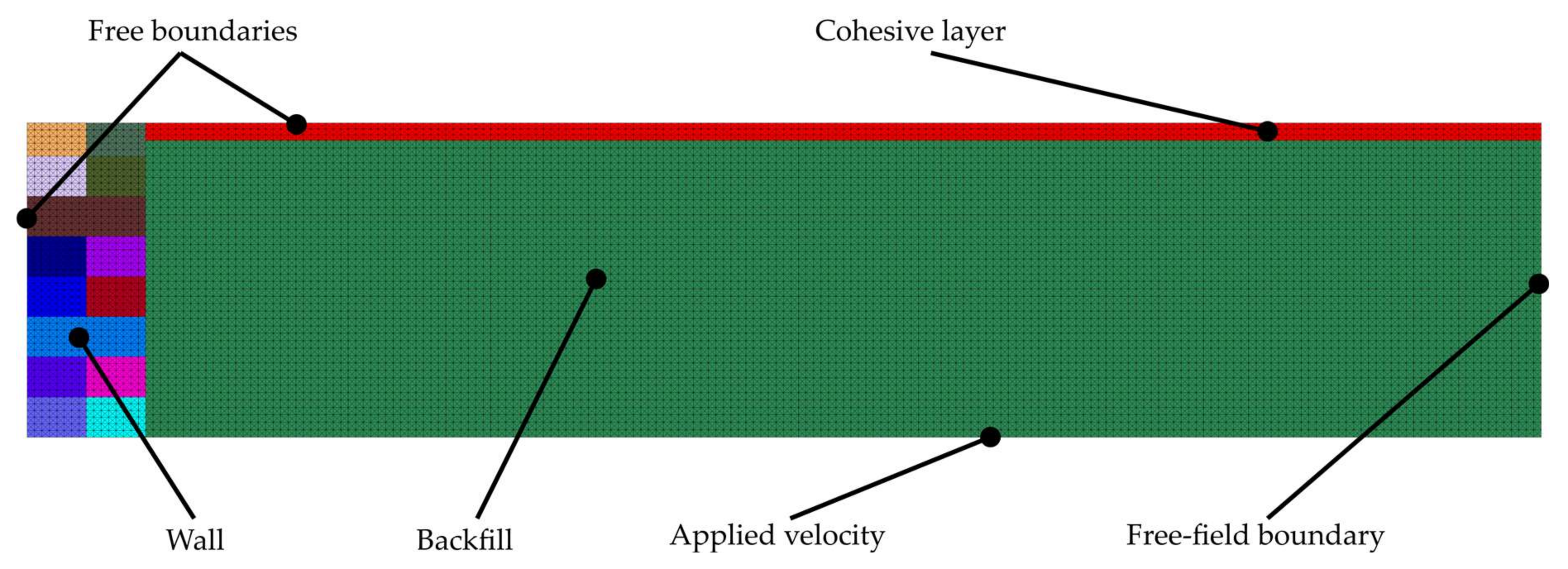
2. Numerical DEM Strategy for Dynamic Simulations
vi(t + Δt/2) = vi(t − Δt/2) + ai(t) × Δt
ui(t + Δt) = ui(t) + vi(t + Δt/2) × Δt
ΔFs = Ac × ks × Δus = Ac × ks × [us(t + Δt) − us(t)]
Fs(t + Δt) = Fs(t) + ΔFs, |Fs| < Fs, max = C × Ac − Fn × tan(φ)
3. Validation of the Model on Scaled-Down Experiments
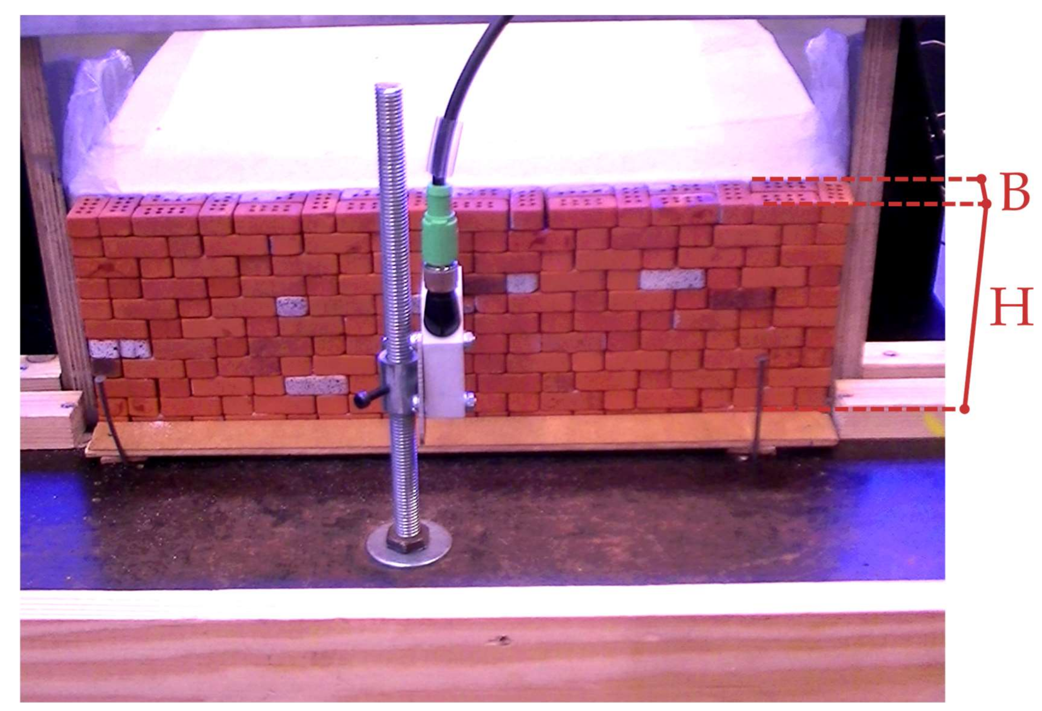
3.1. Experimental Results
3.2. Numerical Parameters of the UDEC Simulations
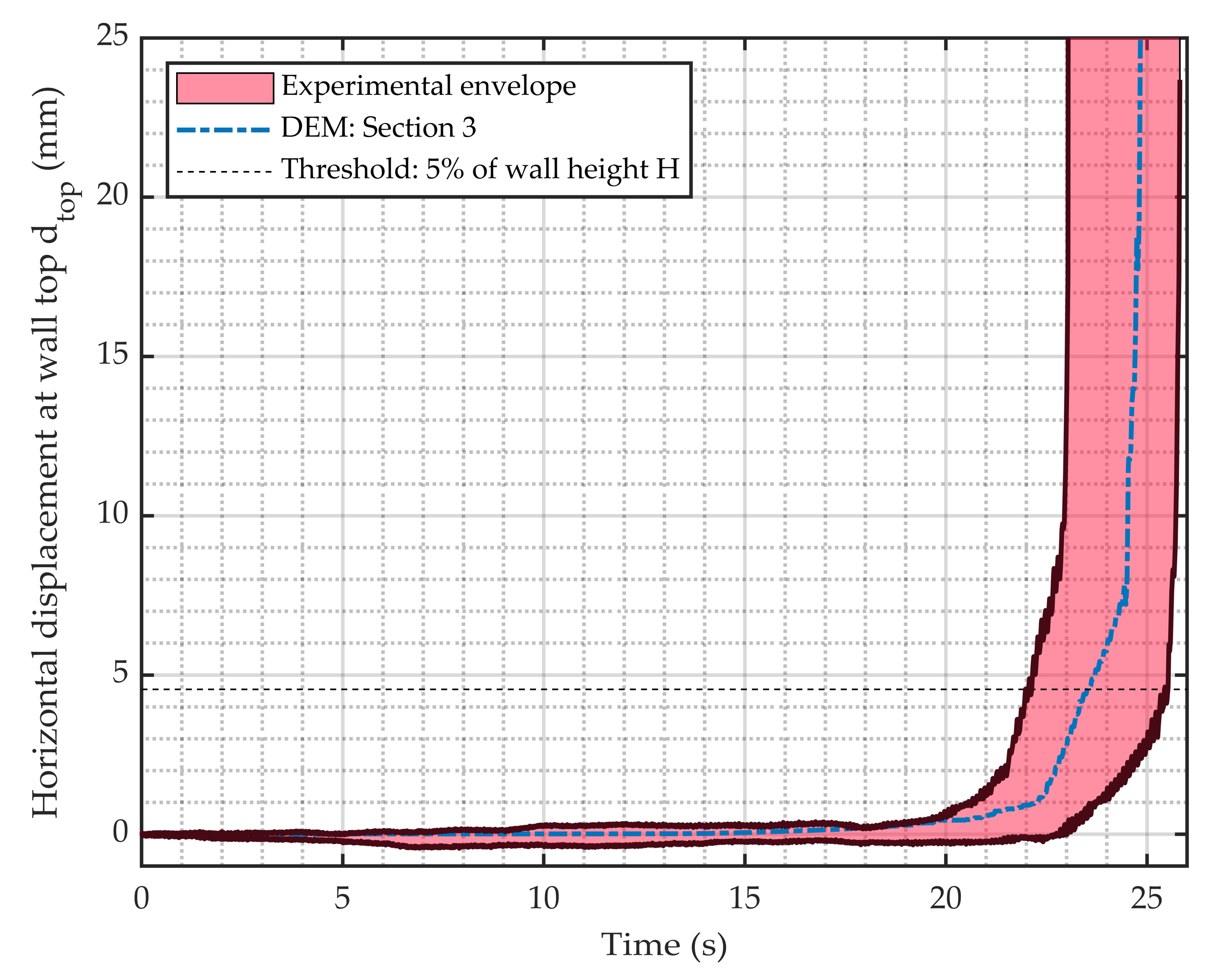
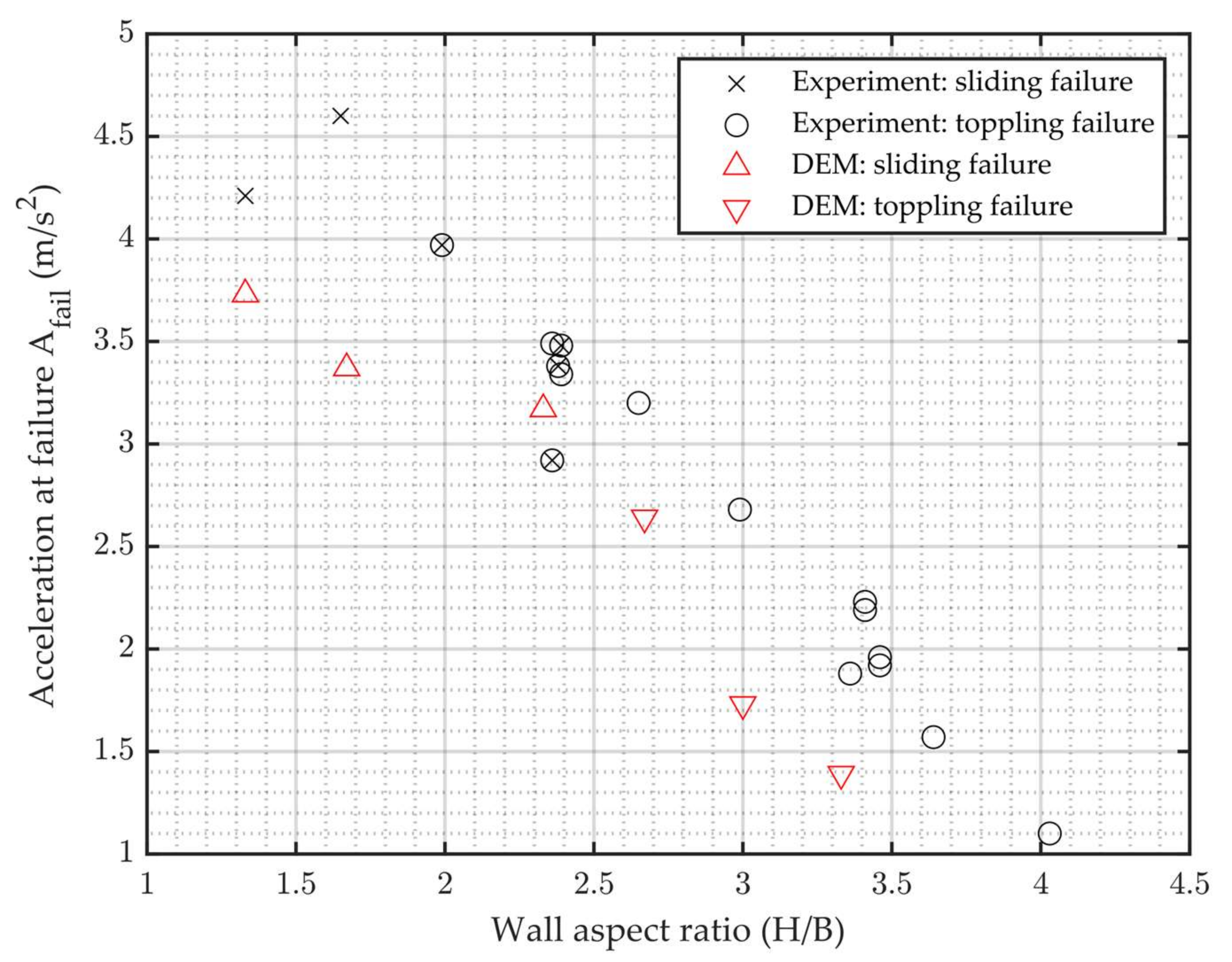
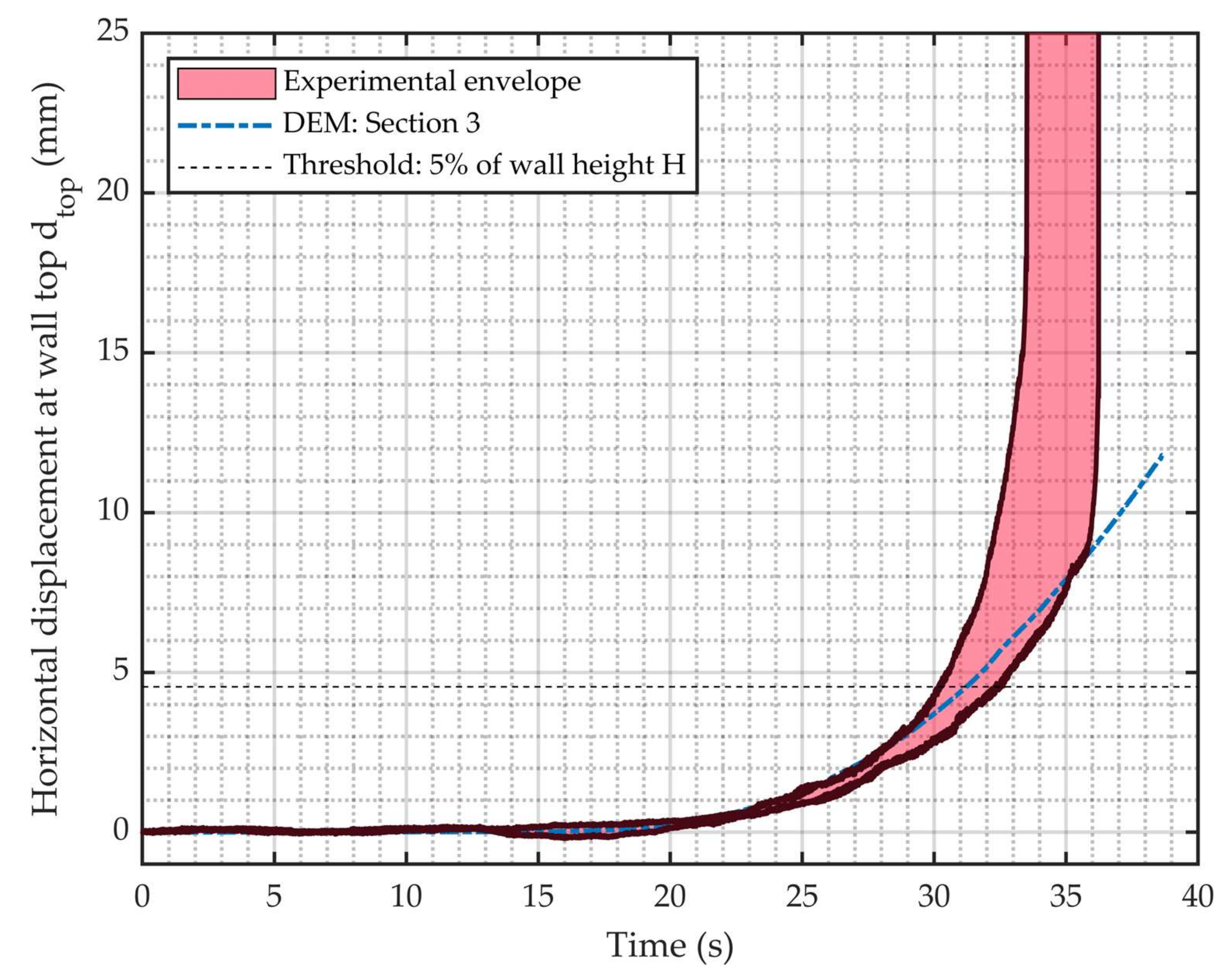
3.3. Validation of the Modelling Strategy
3.4. Effect of the Frequency
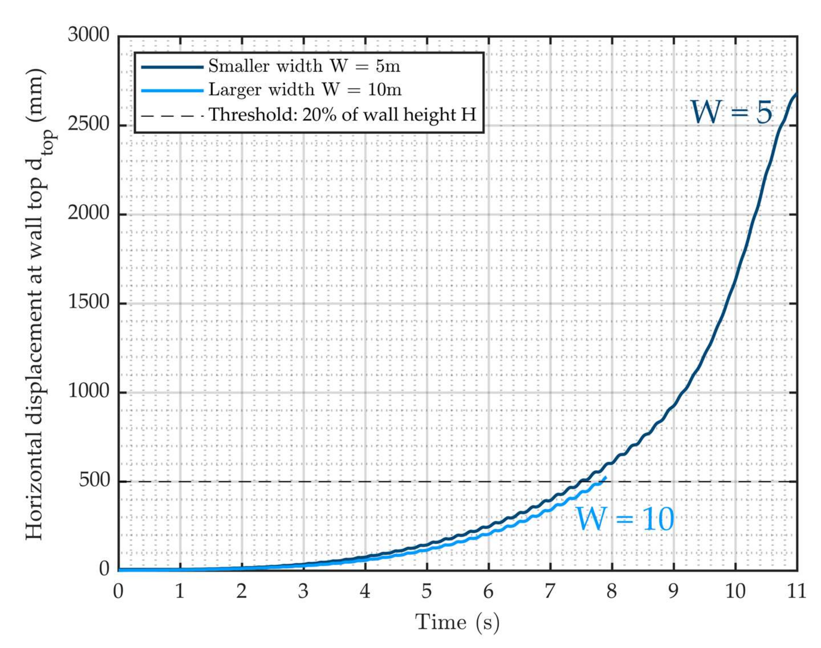
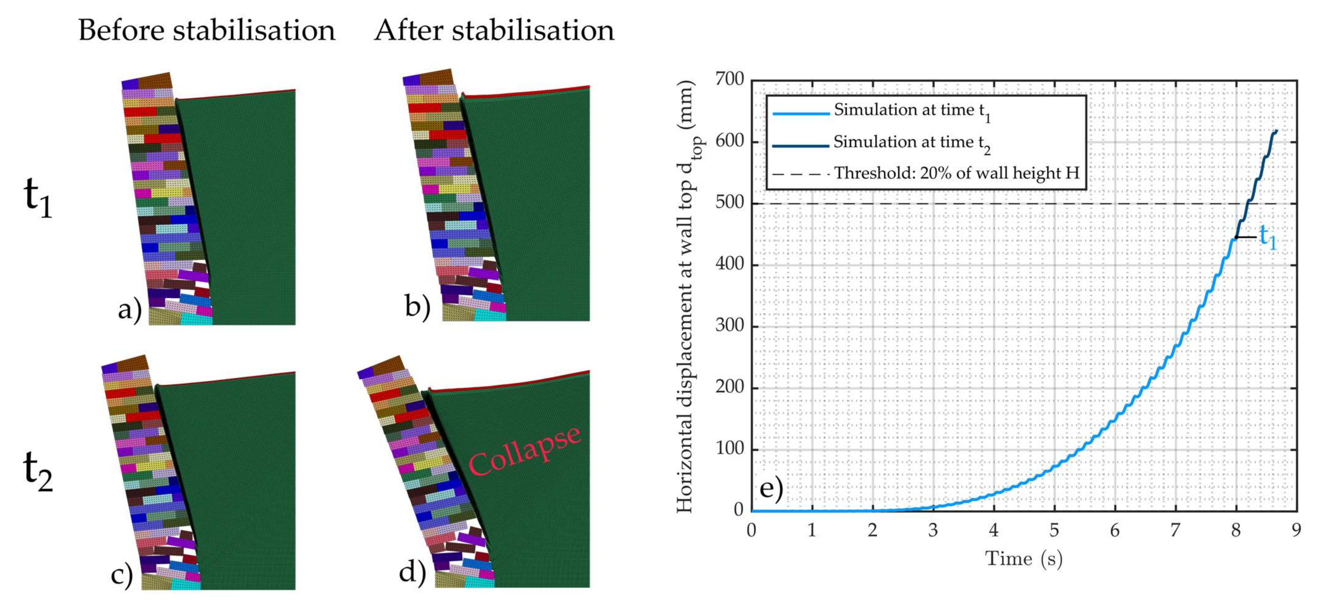
4. Full-Scale Numerical Simulations: Extraction of the Seismic Behaviour Factor
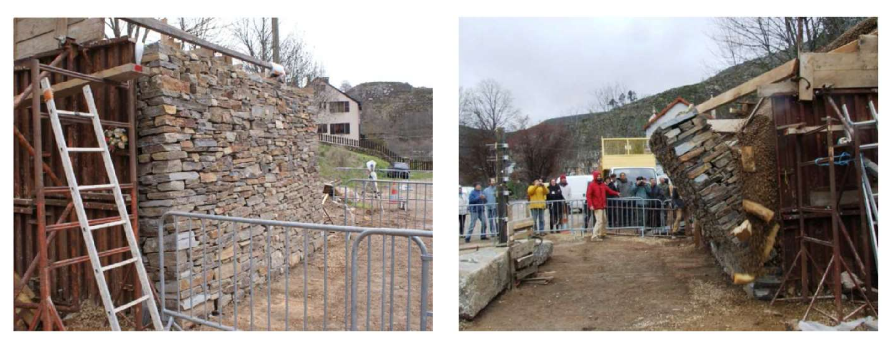
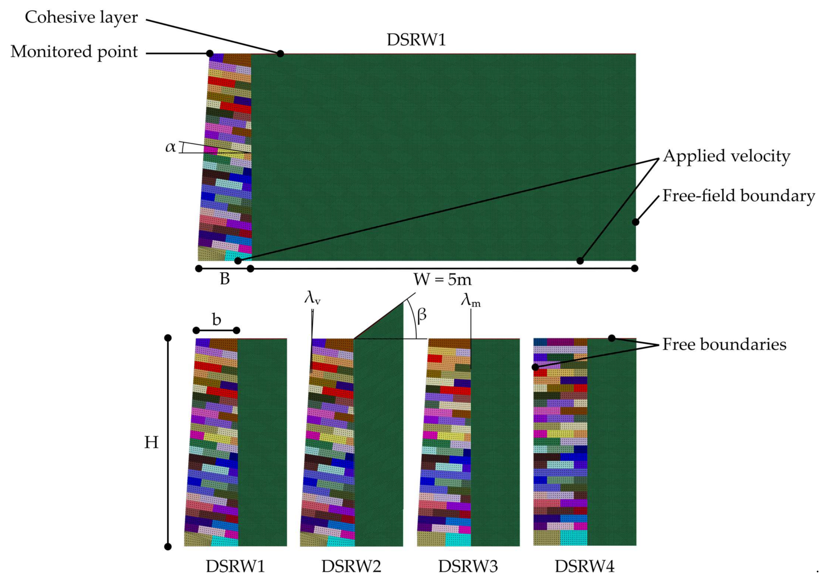
4.1. Description of the Case Study
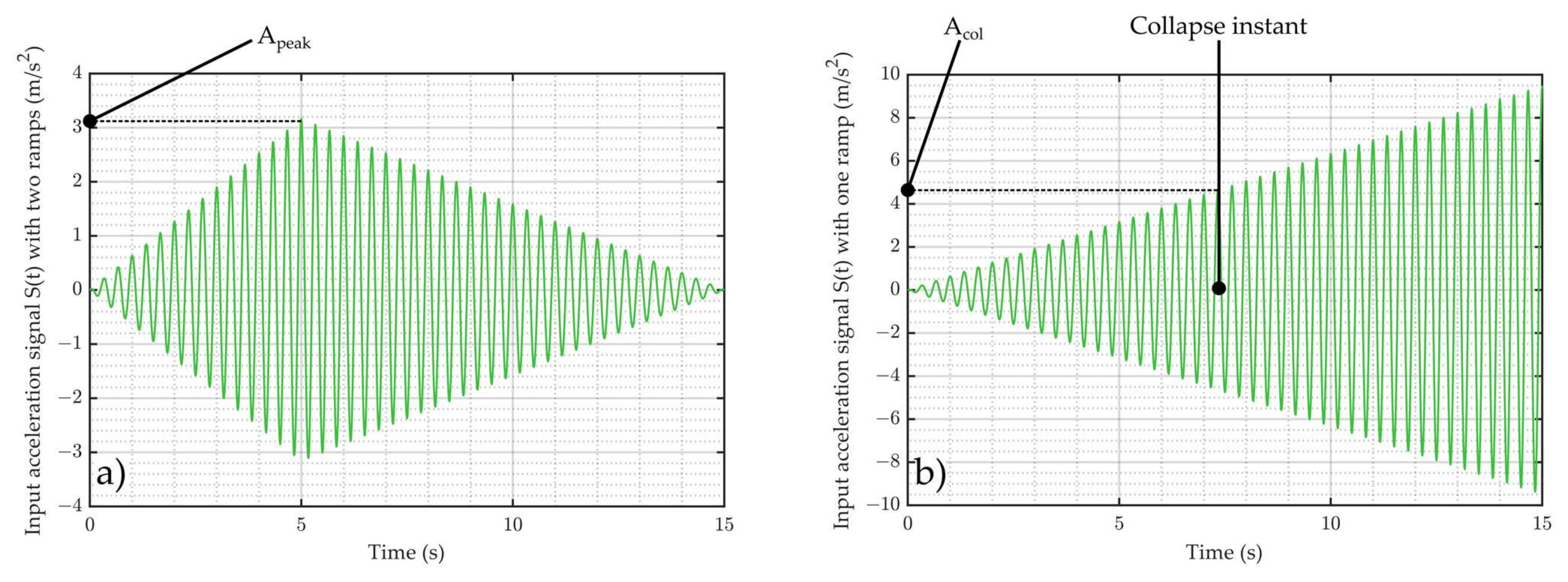
4.2. Dynamic Input Signal
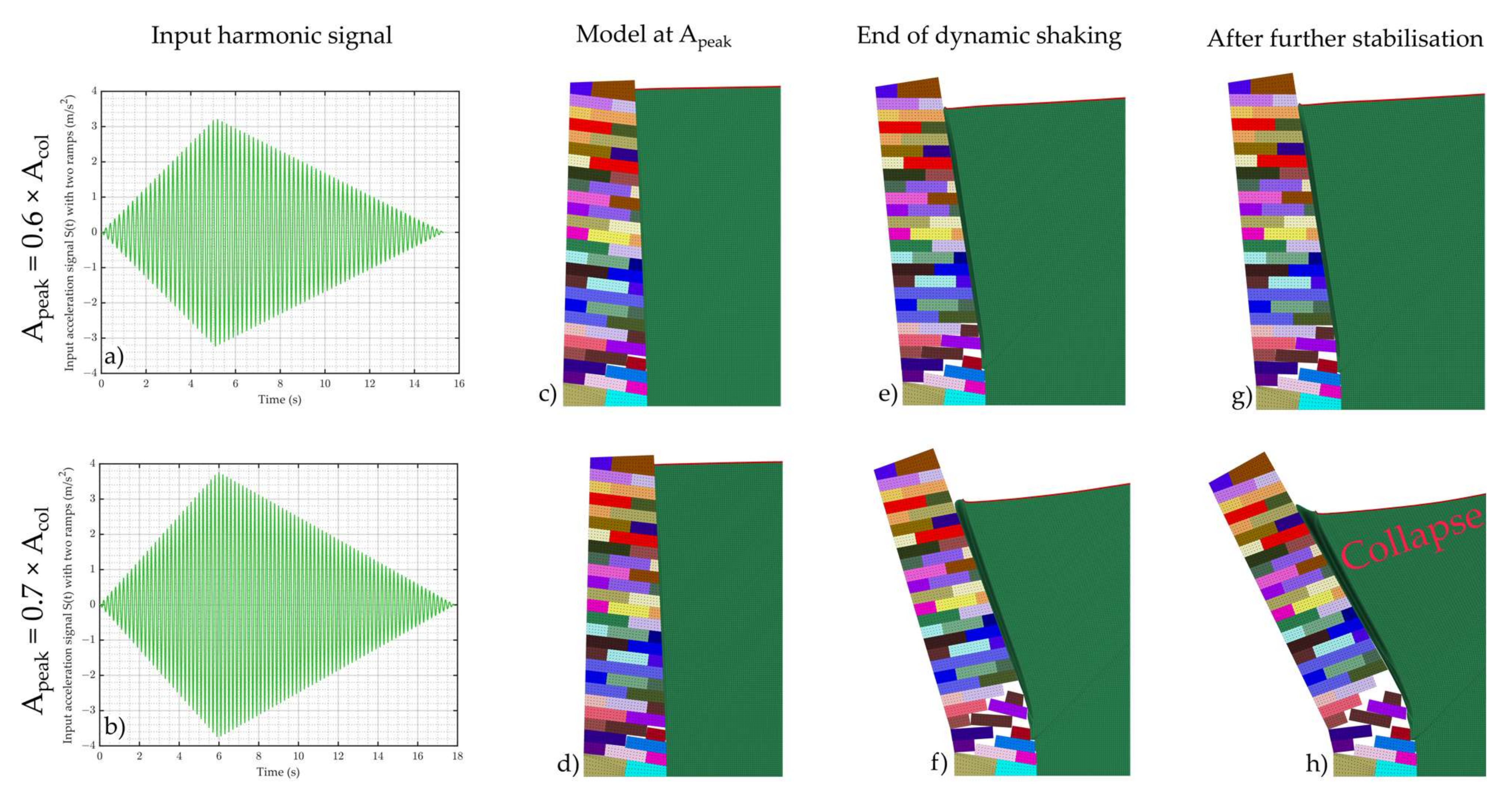
4.3. Different Configurations Tested
4.4. Comparison of Pseudo-Static Predictions and the Estimated Behaviour Factor r
5. Conclusions
Author Contributions
Funding
Institutional Review Board Statement
Informed Consent Statement
Data Availability Statement
Acknowledgments
Conflicts of Interest
References
- Alava, C.; Augeraud, L.; Apavou, S.; Bouskela, D.; Lenoir, C.; Peyrard, M. Murs de Soutènement: Comparaison Environnementale et Financière de Différentes Technologies; Projet de Recherche; Internal Report; Ecole Centrale de Lyon: Lyon, France, 2009. [Google Scholar]
- Preti, F.; Errico, A.; Caruso, M.; Dani, A.; Guastini, E. Dry-stone wall terrace monitoring and modelling. Land Degrad. Dev. 2018, 29, 1806–1818. [Google Scholar] [CrossRef]
- Tarolli, P.; Preti, F.; Romano, N. Terraced landscapes: From an old best practice to a potential hazard for soil degradation due to land abandonment. Anthropocene 2014, 6, 10–25. [Google Scholar] [CrossRef]
- CAPEB; ABPS; Muraillers de Provence; CBPS; CMA84; ENTPE. Pierres Sèches: Guide de Bonnes Pratiques de Construction de Murs de Soutènement; ENTPE: Lyon, France, 2008. [Google Scholar]
- ENTPE; Artisans Bâtisseurs en Pierre Sèche (ABPS); Ecole des Ponts ParisTech; IFSTTAR; Fédération Française du Bâtiment (FFB). Technique de Construction des Murs en Pierre Sèche: Règles Professionnelles; ENTPE: Lyon, France, 2017. [Google Scholar]
- Dickens, J.G.; Walker, P.J. Use of distinct element model to simulate behaviour of dry-stone walls. Struct. Eng. Rev. 1996, 2–3, 187–199. [Google Scholar] [CrossRef]
- Walker, P.; McCombie, P.; Claxton, M. Plane strain numerical model for drystone retaining walls. Proc. Inst. Civ. Eng. Geotech. Eng. 2007, 160, 97–103. [Google Scholar] [CrossRef]
- McCombie, P.F.; Mundell, C.; Heath, A.; Walker, P. Drystone retaining walls: Ductile engineering structures with tensile strength. Eng. Struct. 2012, 45, 238–243. [Google Scholar] [CrossRef] [Green Version]
- Mundell, C.; McCombie, P.; Heath, A.; Harkness, J. Behaviour of drystone retaining structures. Proc. Inst. Civ. Eng. 2010, 163, 3–12. [Google Scholar] [CrossRef] [Green Version]
- Harkness, R.M.; Powrie, W.; Zhang, X.; Brady, K.C.; O’Reilly, M.P. Numerical modelling of full-scale tests on drystone masonry retaining walls. Géotechnique 2000, 50, 165–179. [Google Scholar] [CrossRef]
- Powrie, W.; Harkness, R.M.; Zhang, X.; Bush, D.I. Deformation and failure modes of drystone retaining walls. Géotechnique 2002, 52, 435–446. [Google Scholar] [CrossRef]
- Colas, A.-S.; Morel, J.-C.; Garnier, D. Yield design of dry-stone masonry retaining structures—Comparisons with analytical, numerical, and experimental data. Int. J. Numer. Anal. Methods Geomech. 2008, 32, 1817–1832. [Google Scholar] [CrossRef]
- Alejano, L.R.; Veiga, M.; Taboada, J.; Díez-Farto, M. Stability of granite drystone masonry retaining walls: I. Analytical design. Géotechnique 2012, 62, 1013–1025. [Google Scholar] [CrossRef]
- Villemus, B.; Morel, J.-C.; Boutin, C. Experimental assessment of dry stone retaining wall stability on a rigid foundation. Eng. Struct. 2006, 29, 2124–2132. [Google Scholar] [CrossRef] [Green Version]
- Burgoyne, J. Revetments of retaining walls. Corps R. Eng. Pap. 1853, 3, 154–159. [Google Scholar]
- Colas, A.-S.; Morel, J.-C.; Garnier, D. Assessing the two-dimensional behaviour of drystone retaining walls by full-scale experiments and yield design simulation. Géotechnique 2013, 63, 107–117. [Google Scholar] [CrossRef] [Green Version]
- Le, H.H.; Morel, J.-C.; Colas, A.-S.; Terrade, B.; Garnier, D. Assessing the Three-Dimensional Behaviour of Dry Stone Retaining Walls by Full-Scale Experiments. Int. J. Archit. Herit. 2020, 14, 1373–1383. [Google Scholar] [CrossRef]
- Savalle, N.; Vincens, E.; Hans, S. Pseudo-static scaled-down experiments on dry stone retaining walls: Preliminary implications for the seismic design. Eng. Struct. 2018, 171, 336–347. [Google Scholar] [CrossRef]
- Pulatsu, B.; Kim, S.; Erdogmus, E.; Lourenço, P.B. Advanced analysis of masonry retaining walls using mixed discrete–continuum approach. Proc. Inst. Civ. Eng. Geotech. Eng. 2020, 174, 302–314. [Google Scholar] [CrossRef]
- Oetomo, J.J.; Vincens, E.; Dedecker, F.; Morel, J.-C. Modeling the 2D behavior of dry-stone retaining walls by a fully discrete element method. Int. J. Numer. Anal. Methods Geomech. 2016, 40, 1099–1120. [Google Scholar] [CrossRef]
- Quezada, J.-C.; Vincens, E.; Mouterde, R.; Morel, J.-C. 3D failure of a scale-down dry stone retaining wall: A DEM modelling. Eng. Struct. 2016, 117, 506–517. [Google Scholar] [CrossRef] [Green Version]
- Savalle, N.; Vincens, É.; Hans, S. Experimental and numerical studies on scaled-down dry-joint retaining walls: Pseudo-static approach to quantify the resistance of a dry-joint brick retaining wall. Bull. Earthq. Eng. 2020, 18, 581–606. [Google Scholar] [CrossRef]
- Alejano, L.R.; Veiga, M.; Gómez-Márquez, I.; Taboada, J. Stability of granite drystone masonry retaining walls: II. Relevant parameters and analytical and numerical studies of real walls. Géotechnique 2012, 62, 1027–1040. [Google Scholar] [CrossRef]
- Colas, A.-S.; Morel, J.-C.; Garnier, D. Full-scale field trials to assess dry-stone retaining wall stability. Eng. Struct. 2010, 32, 1215–1222. [Google Scholar] [CrossRef]
- Terrade, B.; Colas, A.-S.; Garnier, D. Upper bound limit analysis of masonry retaining walls using PIV velocity fields. Meccanica 2018, 53, 1661–1672. [Google Scholar] [CrossRef]
- Le, H.H.; Garnier, D.; Colas, A.-S.; Terrade, B.; Morel, J.-C. 3D homogenised strength criterion for masonry: Application to drystone retaining walls. J. Mech. Phys. Solids 2016, 95, 239–253. [Google Scholar] [CrossRef]
- Savalle, N.; Monchal, C.; Vincens, E.; Forcioli, S.; Lourenço, P.B. Static and seismic design of Dry-Stone Retaining Walls (DSRWs) Following Eurocode Standards; 2022; in press. [Google Scholar]
- NF EN 1998-1:2005; Eurocode 8: Design of Structures for Earthquake Resistance—Part 1: General Rules, Seismic Actions and Rules for Buildings. AFNOR: Brussels, Belgium, 2005.
- Newmark, N.M. Effects of earthquakes on dams and embankments. Geotechnique 1965, 15, 139–160. [Google Scholar] [CrossRef] [Green Version]
- Tiwari, R.; Lam, N. Displacement based seismic assessment of base restrained retaining walls. Acta Geotech. 2022, 1–20. [Google Scholar] [CrossRef]
- Conte, E.; Pugliese, L.; Troncone, A. Earthquake-induced permanent displacements of embedded cantilever retaining walls. Géotechnique 2022, online. 1–10. [Google Scholar] [CrossRef]
- NF EN 1998-5:2005; Eurocode 8: Design of Structures for Earthquake Resistance—Part 5: Foundations, Retaining Structures and Geotechnical Aspects. AFNOR: Brussels, Belgium, 2005.
- Savalle, N.; Blanc-Gonnet, J.; Vincens, E.; Hans, S. Dynamic behaviour of drystone retaining walls: Shaking table scaled-down tests. Eur. J. Environ. Civ. Eng. 2020, 1–21. [Google Scholar] [CrossRef]
- Zhang, X.; Koutsabeloulis, N.C.; Hope, S.; Pearce, A. A finite element analysis for the stability of drystone masonry retaining walls. Géotechnique 2004, 54, 57–60. [Google Scholar] [CrossRef]
- Itasca. Universal Distinct Element Code (UDEC): Theory and Background, 7th ed.; Itasca Consulting Group: Minneapolis, MN, USA, 2019. [Google Scholar]
- Lemos, J.V. Discrete Element Modeling of Masonry Structures. Int. J. Archit. Herit. 2007, 1, 190–213. [Google Scholar] [CrossRef]
- Lemos, J.V. Discrete Element Modeling of the Seismic Behavior of Masonry Construction. Buildings 2019, 9, 43. [Google Scholar] [CrossRef] [Green Version]
- Furukawa, A.; Kiyono, J.; Toki, K. Numerical simulation of the failure propagation of masonry buildings during an earthquake. J. Nat. Disaster Sci. 2012, 33, 11–36. [Google Scholar] [CrossRef] [Green Version]
- Matasović, N.; Vucetic, M. Cyclic characterization of liquefiable sands. J. Geotech. Eng. 1993, 119, 1805–1822. [Google Scholar] [CrossRef]
- Amirouche, N. Dispositifs absorbants à base de matériaux à double porosité dans des champs acoustiques complexes. Ph.D. Thesis, Ecole Nationale des Travaux Publics de l’Etat (ENTPE), Lyon, France, 2008. [Google Scholar]
- Giuffrè, A. A mechanical model for statics and dynamics of historical masonry buildings’. In Protection of the Architectural Heritage against Earthquakes; Springer: Berlin/Heidelberg, Germany, 1996; pp. 71–152. [Google Scholar]
- de Felice, G. Out-of-plane seismic capacity of masonry depending on wall section morphology. Int. J. Archit. Herit. 2011, 5, 466–482. [Google Scholar] [CrossRef]
- Colas, A.-S. Mécanique des Murs de Soutenement en Pierre Sèche: Modélisation par le Calcul à la Rupture et Expérimentation échelle 1’. Ph.D. Thesis, Ecole Nationale des Travaux Publics de l’Etat (ENTPE), Lyon, France, 2009. [Google Scholar]
- Mauro, A.; de Felice, G.; DeJong, M.J. The relative dynamic resilience of masonry collapse mechanisms. Eng. Struct. 2015, 85, 182–194. [Google Scholar] [CrossRef]
- Vassiliou, M.F.; Makris, N. Analysis of the rocking response of rigid blocks standing free on a seismically isolated base. Earthq. Eng. Struct. Dyn. 2012, 41, 177–196. [Google Scholar] [CrossRef]
- DeJong, M.J.; de Lorenzis, L.; Adams, S.; Ochsendorf, J.A. Rocking stability of masonry arches in seismic regions. Earthq. Spectra 2008, 24, 847–865. [Google Scholar] [CrossRef]
- Gobbin, F.; de Felice, G.; Lemos, J.V. Numerical procedures for the analysis of collapse mechanisms of masonry structures using discrete element modelling. Eng. Struct. 2021, 246, 113047. [Google Scholar] [CrossRef]
- Hans, S. Génie Parasismique; IFSTTAR: Paris, France, 2013. [Google Scholar]
- Lee, W.H.K.; Bennett, R.E.; Meagher, K.L. A Method of Estimating Magnitude of Local Earthquakes from Signal Duration; US Department of the Interior Geological Survey: Menlo Park, CA, USA, 1972. [Google Scholar]
- Bisztricsany, E. A new method for the determination of the magnitude of earthquakes. Geofiz. Kozlemen 1958, 7, 69–96. [Google Scholar]
- Tsumura, K. Determination of earthquake magnitude from total duration of oscillation. Bull. Earthquake Res. Inst. Tokyo Univ. 1967, 45, 18. [Google Scholar]
- Crosson, R.S. Small earthquakes, structure, and tectonics of the Puget Sound region. Bull. Seismol. Soc. Am. 1972, 62, 1133–1171. [Google Scholar]
- Akkar, S.; Sandıkkaya, M.A.; Şenyurt, M.; Azari Sisi, A.; Ay, B.O.; Traversa, P.; Douglas, J.; Cotton, F.; Luzi, F.; Hernandez, B.; et al. Reference database for seismic ground-motion in Europe (RESORCE). Bull. Earthq. Eng. 2014, 12, 311–339. [Google Scholar] [CrossRef] [Green Version]
- Durand, C. Stabilité des digues sous chargement sismique: Vers une nouvelle génération de méthodes simplifiées. Ph.D. Thesis, Université Grenoble Alpes, Grenoble, France, 2018. [Google Scholar]
- Samayoa, J.; Baraccani, S.; Pieraccini, L.; Silvestri, S. Seismic Behavior of One-Storey Gabion-Box Walls Buildings. Front. Built Environ. 2018, 4, 7. [Google Scholar] [CrossRef] [Green Version]
- Savalle, N.; Vincens, E.; Lourenço, P.B. Pseudo-static analytical model for the static and seismic stability of dry stone retaining walls. In Proceedings of the 7th International Conference on Geotechnical Research and Engineering, Lisbon, Portugal, 10–12 April 2022. [Google Scholar]


| Units | Backfill | Wall–Backfill Interface | |
|---|---|---|---|
| Volumetric properties | |||
| Unit weight γ (kN/m3) [33] | 14.4 | 15.4 | - |
| Elastic modulus E (MPa) | 1000 | 10 | - |
| Poisson ratio ν | 0.2 | 0.3 | - |
| Friction angle φ (°) [33] | - | 45 | - |
| Interface properties | |||
| Friction angle φ (°) [33] | 32 | - | 32 |
| Normal stiffness kn (Pa/m3) | 2.6 × 10¹² | - | 3.0 × 10¹⁰ |
| Tangential stiffness ks (Pa/m3) | 2.6 × 10¹² | - | 3.0 × 10¹⁰ |
| Numerical parameters | |||
| Timestep Δt (s) | ≈1 × 10⁻⁶ | ||
| Rayleigh viscous damping ξ | 10% at 10Hz |
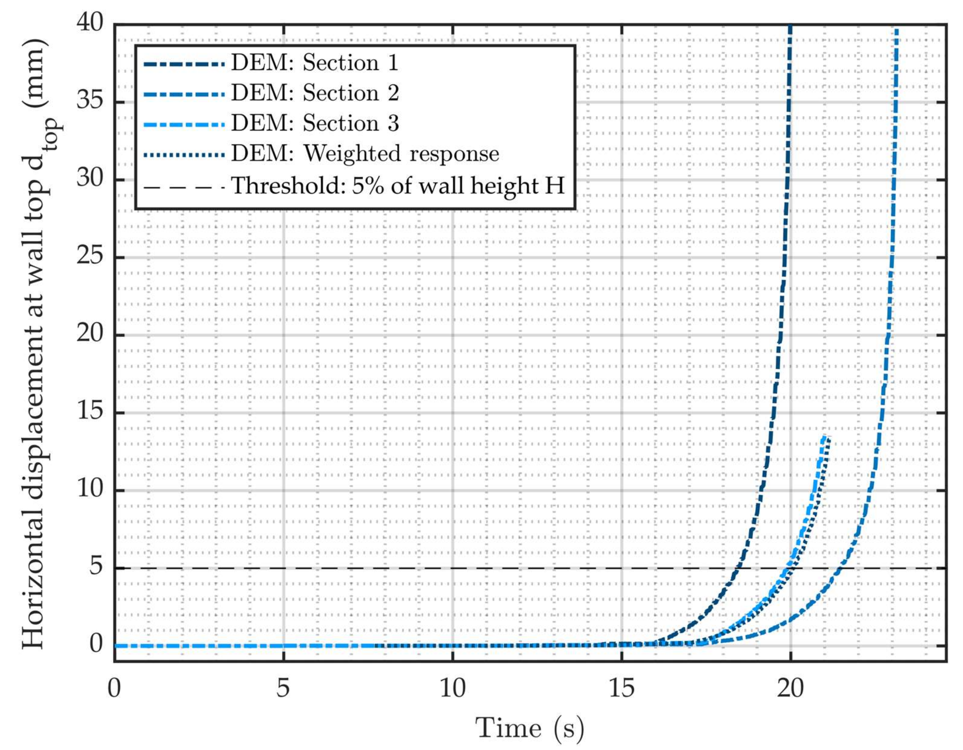
| Section No. | Proportion | Time for dtop = 5 mm (s) |
|---|---|---|
| 1 | 7/23 | 18.4 |
| 2 | 7/23 | 21.5 |
| 3 | 7/23 | 19.9 |
| 4 | 2/23 | 21.5 |
| Weighted average | 20.1 | |
| Wall Slenderness (H/B) | Exp. Afail (m/s2) | Exp. Failure Mode | Num. Afail (m/s2) | Num. Failure Mode | Error (%) |
|---|---|---|---|---|---|
| H/B = 1.3 | 4.2 | S | 3.7 | S | −11% |
| H/B = 1.7 | 4.6 | S | 3.4 | S | −27% |
| H/B = 2.3 | 3.3 | S/T | 3.2 | S | −5% |
| H/B = 2.7 | 3.2 | T | 2.6 | T | −18% |
| H/B = 3 | 2.7 | T | 1.7 | T | −35% |
| H/B = 3.3 | 2.0 | T | 1.4 | T | −32% |
| Mean | −21% |
| Backfill Friction Angle φ (°) | 45° | 50° | 55° |
|---|---|---|---|
| Error compared with experiment (%) | −18% | −13% | −10% |
| Geometrical Parameters | Original Wall “C3s” | DSRW1 | DSRW2 | DSRW3 | DSRW4 |
|---|---|---|---|---|---|
| Height H (m) | 2.5 | 2.5 | 2.5 | 2.5 | 2.5 |
| Width at base B (m) | 0.7 | 0.7 | 0.7 | 0.7 | 0.7 |
| Width at top b (m) | 0.55 | 0.55 | 0.55 | 0.55 | 0.7 |
| Internal batter λm (%) | 0 | 0 | 0 | 0 | 0 |
| External batter λv (%) | 6 | 6 | 6 | 6 | 0 |
| Bed inclination α (º) | 9.1 | 9.1 | 9.1 | 3.4 | 0 |
| Backfill slope β (º) | 32.6 | 0 | 32.6 | 0 | 0 |
| Mechanical Parameters | Units | Backfill [43] | Interface |
|---|---|---|---|
| Volumetric properties | |||
| Unit weight (kN/m3) [43] | 20.0 | 14.9 | - |
| Elastic modulus E (MPa) | 10,000 | 92.7 | - |
| Poisson ratio ν | 0.3 | 0.22 | - |
| Friction angle φ (°) | - | 37.7 | - |
| Interface properties | |||
| Friction angle φ (°) [43] | 25.0 | 37.7 | 37.7 |
| Normal stiffness kn (Pa/m3) | 2.8 × 10¹² | - | 2.9 × 10¹⁰ |
| Tangential stiffness ks (Pa/m3) | 2.8 × 10¹² | - | 2.9 × 10¹⁰ |
| Numerical parameters | |||
| Timestep Δt (s) | ≈ 5 × 10⁻⁶ | ||
| Rayleigh viscous damping ξ | 10% |
| DSRW Name | DSRW1 | DSRW2 | DSRW3 | DSRW4 | ||||
|---|---|---|---|---|---|---|---|---|
| Frequency (Hz) | 3Hz | 5Hz | 10Hz | 5Hz | 5Hz | 5Hz | 5Hz | 5Hz |
| Vertical acceleration | - | - | - | in-phase | opposition | - | - | - |
| tcol (s) | 7.6 | 8.5 | 9.5 | 8.9 | 8.6 | 9.4 | 8.3 | 8.5 |
| Acol (m/s2) | 4.83 | 5.38 | 6.03 | 5.34 | 5.19 | 1.83 | 5.06 | 4.63 |
| DSRW Geometry | DSRW1 | DSRW2 | DSRW3 | DSRW4 | ||||
|---|---|---|---|---|---|---|---|---|
| Frequency (Hz) | 3Hz | 5Hz | 10Hz | 5Hz | 5Hz | 5Hz | 5Hz | 5Hz |
| Vertical acceleration | - | - | - | in-phase | opposition | - | - | - |
| Acol (m/s2) | 4.83 | 5.38 | 6.03 | 5.34 | 5.19 | 1.83 | 5.06 | 4.63 |
| Apeak = 0.6 × Acol (m/s2) | 2.90 | 3.23 | 3.62 | 3.21 | 3.11 | 1.10 | 3.04 | 2.78 |
| Apseudo (m/s2) | 1.58 | 1.58 | 1.58 | 1.50 | 1.50 | 0.49 | 1.36 | 1.52 |
| r = Apeak/Apseudo | 1.83 | 2.04 | 2.29 | 2.14 | 2.07 | 2.26 | 2.00 | 2.04 |
Publisher’s Note: MDPI stays neutral with regard to jurisdictional claims in published maps and institutional affiliations. |
© 2022 by the authors. Licensee MDPI, Basel, Switzerland. This article is an open access article distributed under the terms and conditions of the Creative Commons Attribution (CC BY) license (https://creativecommons.org/licenses/by/4.0/).
Share and Cite
Savalle, N.; Vincens, E.; Hans, S.; Lourenço, P.B. Dynamic Numerical Simulations of Dry-Stone Retaining Walls: Identification of the Seismic Behaviour Factor. Geosciences 2022, 12, 252. https://0-doi-org.brum.beds.ac.uk/10.3390/geosciences12060252
Savalle N, Vincens E, Hans S, Lourenço PB. Dynamic Numerical Simulations of Dry-Stone Retaining Walls: Identification of the Seismic Behaviour Factor. Geosciences. 2022; 12(6):252. https://0-doi-org.brum.beds.ac.uk/10.3390/geosciences12060252
Chicago/Turabian StyleSavalle, Nathanaël, Eric Vincens, Stéphane Hans, and Paulo B. Lourenço. 2022. "Dynamic Numerical Simulations of Dry-Stone Retaining Walls: Identification of the Seismic Behaviour Factor" Geosciences 12, no. 6: 252. https://0-doi-org.brum.beds.ac.uk/10.3390/geosciences12060252