An Overview of Opportunities for Machine Learning Methods in Underground Rock Engineering Design


Department of Civil Engineering, Lassonde School of Engineering, York University, Toronto, ON M3J 1P3, Canada
*
Author to whom correspondence should be addressed.
Geosciences 2019, 9(12), 504; https://0-doi-org.brum.beds.ac.uk/10.3390/geosciences9120504
Submission received: 19 November 2019
/
Revised: 27 November 2019
/
Accepted: 28 November 2019
/
Published: 2 December 2019
Abstract
:Machine learning methods for data processing are gaining momentum in many geoscience industries. This includes the mining industry, where machine learning is primarily being applied to autonomously driven vehicles such as haul trucks, and ore body and resource delineation. However, the development of machine learning applications in rock engineering literature is relatively recent, despite being widely used and generally accepted for decades in other risk assessment-type design areas, such as flood forecasting. Operating mines and underground infrastructure projects collect more instrumentation data than ever before, however, only a small fraction of the useful information is typically extracted for rock engineering design, and there is often insufficient time to investigate complex rock mass phenomena in detail. This paper presents a summary of current practice in rock engineering design, as well as a review of literature and methods at the intersection of machine learning and rock engineering. It identifies gaps, such as standards for architecture, input selection and performance metrics, and areas for future work. These gaps present an opportunity to define a framework for integrating machine learning into conventional rock engineering design methodologies to make them more rigorous and reliable in predicting probable underlying physical mechanics and phenomenon.
1. Introduction
The study of rock mechanics encompasses the theoretical and applied science of the mechanical behaviour of rock in response to its physical environment and was formalized as a field of study in the 1960s [1]. Due to the high degree of variability in natural materials, a precise rock engineering design within a narrow tolerance is difficult to produce. Experience and expert knowledge are heavily relied upon in rock engineering practice and empirical design charts have become prolific for preliminary stage design. Numerical modelling methods such as continuum and discrete methods, are also conventional tools in rock engineering design. These methods represent important tools for understanding rock mass behaviour and predicting its response to its environment and changes in in situ stress conditions. In practice, it is often difficult to integrate all the data collected into empirical and numerical models effectively due to time and budget constraints, as well as limitations in how constitutive behaviour is defined. Furthermore, it is sometimes not feasible to collect the quality and quantity of data needed, so extrapolation and interpolation techniques are often used.
Prior to the advent of “big data” and advances in machine learning, it was appropriate to base rock engineering design primarily on empirical data and expert knowledge because the geology, discontinuity, and in situ stress data available for projects were generally sparse. Now, increasing amounts of some forms of data such as displacements and pore water pressures, are being collected relatively inexpensively, while others are still infrequently collected because of the complexity and cost of the measurement methods, such as those used for stress measurement. Herein lies an opportunity to integrate machine learning into the existing rock engineering best practices to evaluate datasets more efficiently and to maximize the value (or information) extracted from the data. Machine learning algorithms are especially powerful because simultaneous hypotheses can be tested much quicker than by a human being [2]. This frees up the expert user or engineer to devote their judgment to selecting inputs and validating outputs in a more rigorous way, rather than manipulating data, which can be more time consuming and poses the risk of introducing bias.
Although machine learning has been used in other fields that rely heavily on numerical modelling, such as flood forecasting, for over 20 years [3], comparatively it is in its infancy in rock engineering applications. Some professionals in the mining industry believe the community is reluctant to accept data-driven methods because they are not as interpretable as applying conventional design criteria determined by previous experience and empirical evidence [4]. Work is being done to produce scientifically interpretable data-driven models [5], however, these frameworks have not migrated into engineering practice yet. Expert judgment is given much credence in the rock engineering industry, and empirical relationships form the foundation of fundamental rock engineering methods [6].
The progression of the design process is constrained by the analysis of the data that is collected. Machine learning algorithms have the potential to ease the burden of data analysis. If geotechnical professionals are able to predict geomechanical events or behaviours earlier and more accurately, this could translate to increased safety for underground personnel as well as cost savings in terms of reducing equipment loss, increasing efficiency of resource extraction or excavation rates, and minimizing delays and shutdowns.
This paper aims to summarize the most common practices in rock engineering design and presents the opportunities for integrating machine learning into existing geomechanical design frameworks. It also presents a review of common machine learning algorithms and how they are currently being applied to rock engineering problems in the literature, as well as future opportunities for data-driven approaches.
2. Current Practices in Rock Engineering Design
The inherent variability associated with natural materials makes standardization across geomechanical design processes difficult. Recent work to develop a geomechanical design framework has resulted in the publication of Eurocode 7 [7]. This code provides guidelines for tunnelling and underground excavations using a limit state approach, however, in general, customized designs are developed for most projects. Two of the most common categories of design approaches used in rock engineering design are: (i) empirical methodologies, and (ii) numerical modelling. These usually fall into a workflow together depending on the stage of the design, from prefeasibility to detailed design. Empirical design recommendations are often taken as a first estimate and are then verified and updated using the appropriate numerical tools, which are based on the geometry and complexity of the problem. For both these approaches, rock engineers use their judgement to combine numerical data (e.g., rock mass properties, stress conditions, pore water pressure) and categorical data (e.g., geological mapping, discontinuity conditions) into an empirical or numerical framework. As context for the remainder of this paper, both categories of conventional methodologies are briefly described below.
2.1. Empirical Design
In the early stages of conventional rock engineering design, it is common to turn to an established empirical rock support recommendation method to inform the design. The designed rock support may consist of a combination of rock or cable bolts, shotcrete, steel mesh, steel straps, concrete liner segments, etc. These methods are generally dependent on the size of the excavation and the quality of the rock mass and are used only as a first estimate followed by analytical or numerical methods to verify the design. It is typical to use multiple empirical methods and a range of input parameters representing the best- and worst-case to obtain a range of rock support recommendations. In this section, two common empirical rock support methodologies are described: the Rock Mass Rating (RMR) [8] and the Q Tunnelling Index [9]. These systems have been in wide use in the tunnelling and mining industries for 45 years, and have become engrained in standard rock engineering practice [10]. However, previous researchers [10] advocate for exercising caution when using these empirical systems, and for practicing engineers to use them in the spirit for which they were developed—to assist with the design of excavations, but not as the sole tool for designing underground support. Both these classification systems result in a recommended category for rock support, which is meant to encompass the range of rock mass conditions found within that category.
2.1.1. Empirical Support Recommendation—Rock Mass Rating
Bieniawski was among the first to assert that no single index, such as Deere’s Rock Quality Designation [11], was enough to capture that aggregate behaviour of the rock, and so developed the Rock Mass Rating (RMR) system [8] to combine several measureable parameters. This system is the sum of five basic parameters to arrive at a score ranging from 0 to 100:
- Strength of intact rock
- Rock Quality Designation (RQD) [11]
- Spacing of joints
- Condition of joints
- Groundwater conditions
This information is obtained through field mapping and site investigations. The site engineer or geologist collects a score for each of the parameters using the scoring scheme set out by Bieniawski [8]. Statistical analysis is conducted to determine the appropriate value, or more likely values, for each parameter and then sums them to obtain an RMR. The RMR corresponds to a rock quality categorisation that ranges from very good to very poor rock with five classes overall based on a linear relationship with the RMR value. Bieniawski created support guidelines based on the quality of the rock mass i.e., the RMR value and the stress condition the excavation is exposed to [8]. For example, low-stress environments only require heavy support if the rock is of poor quality.
2.1.2. Empirical Support Recommendation—Q Tunnelling Index
The Q Tunnelling Index was developed primarily to predict the appropriate support for tunnels [9] and is defined by multiplication of three quotients: the rock block size, the roughness and frictional resistance, and a stress quotient. As with RMR, the parameters are collected during the site investigation stage of a project and subsequently, a statistical analysis is performed to determine the most representative value or values. The Q Tunnelling Index is a value that ranges from 0.001 to 1000, and the formula is given in Equation (1).
where:
- RQD = Rock Quality Designation [11]
- Jn = Number of joint/fracture sets
- Jr = Roughness of most unfavourable joints
- Ja = Alteration or infilling of joints
- Jw = Water inflow
- SRF = Stress reduction factor, quantifies stress conditions
The major difference between the Q Tunnelling Index support recommendation and others (such as RMR) is the inclusion of a parameter called the equivalent dimension, which uses an excavation support ratio to modify the span or width of the underground opening to capture a factor of safety correlating to the end use of the tunnel.
2.2. Numerical Methods
Numerical modelling is crucial for understanding fundamental intact rock and rock mass behaviour, assessing rock-structure interactions and completing rock engineering designs [12]. These methods offer the tools to capture the mechanisms that are causing observed phenomena in a rock mass or intact rock sample, and subsequently incorporate them into the design. Choosing inputs, geometry, boundary and stress conditions, among other defining aspects of a numerical model, requires significant engineering judgement and the combination of qualitative and quantitative site observations.
A typical approach is to use the back analysis of numerical models to calibrate their behaviour against observed site conditions. These calibrated models are then used to forward predict the excavation behaviour as the excavation is advanced, or as a new excavation is being designed in the same rock mass but at a different location [13]. Figure 1 illustrates this process, summarized as follows:
- Site observations
- Measurements and model calibration
- Conceptual translation of the calibrated behaviour to the new site location
- Comparison with empirical approaches [14] to validate the new design.
For example, the observed overbreak or damage beyond the designed diameter of a tunnel can be back analyzed using a numerical modelling approach. Individual parameters such as tunnel depth, are manipulated independently of the other input variables in order to calibrate them, by taking measurements along the tunnel axis at multiple locations, for example. This calibration process ensures that a robust set of input parameters are determined based on their individual impacts on the measured site conditions at a variety of locations along the tunnel alignment. The empirical knowledge from the tunnel site is translated conceptually to the new site in order to understand what similarities and differences may exist. With this conceptual understanding, a variety of models of the new site can be developed and the results compared to other empirical approaches, such as the damage depth prediction of Diederichs [14].
The most common numerical methods for rock engineering problems are [12]:
- Continuum methods—finite element modelling (FEM), finite difference modelling (FDM), boundary element modelling (BEM).
- Discrete methods—discrete element modelling (DEM), discrete fracture network (DFN) modelling.
- Hybrid continuum/discrete methods.
The choice between methods is made based primarily on the scale of the problem and the geometry of the discontinuity or fracture system in the rock mass [19]. Continuum methods are most appropriate when a detachment of discrete blocks is not a significant factor. Discrete methods are generally chosen when the number of fractures is too large to treat the rock mass as a continuum with fracture elements, or if discrete block detachment is anticipated. Hybrid models are selected to avoid the pitfalls of each of the former two approaches. Each of these methods, their applications and limitations are briefly introduced.
2.2.1. Continuum Methods
The basic concept for continuum methods is to discretize the material being modelled into a grid governed by partial differential equations. The partial differential equations at the grid points are in close enough spatial proximity that the errors introduced between them are insignificant and thus, acceptable.
The FDM is the most direct way to discretize a continuum, where points in space are replaced with discrete equations called finite difference equations. These equations are used to calculate displacement, strain and stress in the material in response to conditional changes in the rock mass [20]. Solutions are formulated at grid points at the local scale, so no global matrix inversion is required, thus saving computational time and intensity. Complex constitutive behaviour can be captured without iterative solutions. However, FDM is inflexible with respect to fractures, complex boundary conditions and material heterogeneity. FDM was historically unsuitable for rock mechanics problems due to these limitations, however, advancements in irregular grid shapes gave rise to related Finite Volume Modelling (FVM) techniques [12]. FVM is more flexible in handling heterogeneity and boundary conditions and has been regarded as the bridge between FDM and FEM [17]. Commonly used commercial FDM software includes FLAC in two-dimensions and FLAC3D in three-dimensions [17].
FEM is the most widely applied numerical method in science and engineering [12]. FEM also involves discretizing a continuum into a grid, however, here, the material is subdivided into parts called finite elements. The partial differential equation at each element is informed by the elements adjacent to it, allowing FEM to handle heterogeneity, plasticity and deformation, complex boundary conditions, in situ stresses and gravity [21]. However, detachment of the elements is not permitted since these models are based on continuum assumptions. The treatment of fractures has been the largest limitation of FEM in the past, and modern software packages include special algorithms to overcome this. Commercial FEM software available are RS2 [22], SIGMA/W [23], Plaxis 2D [24] and ABAQUS [25], while open source options include Adonis [26], OpenSees [27] and Code-Aster [28].
BEM differs from FDM and FEM in that it first seeks an approximate global solution. Initially, BEM was developed for underground stress and deformation analysis, soil-structure interactions, groundwater flow and fracturing processes [12]. BEM approximates the solution of a partial differential equation inside an element by looking to the solution on the boundary and using that to inform the solution inside the element [29]. The main advantage of BEM over FDM or FEM is the simpler mesh generation and decreased computational expense. However, BEM is less efficient than FEM in handling material heterogeneity and plasticity. BEM has been used for: stress analysis of underground excavations, dynamic problems, back analysis of in situ and elastic properties, and borehole permeability tests [12]. Commercially available BEM software includes Examine2D [30] and Map3D [31], while open-source BEM libraries are also available [32].
2.2.2. Discrete Methods
Rock mechanics is one of the fields that originated Discrete Element Method (DEM) modelling, because highly fractured rock masses are not easily described mechanistically by a continuum approach. In discrete element approaches, the material is treated as an assemblage of rigid or deformable blocks or particles, the contacts between which are updated during the modelling process [12]. DEM solutions combine implicit and explicit formulations, based on FEM and FDM discretization, respectively. The main difference between DEM and continuum approaches is that the contacts between the elements are continuously changing, while they remain static for the latter. DEM methods are computationally demanding, however, they offer an advantage when the rock mass experiences loss of continuity (from progressive failure, for example), as continuum constitutive models are inappropriate in that case [33]. DEM methods have been popular for modelling a variety of rock engineering problems including: underground works, rock dynamics, rock slopes, laboratory tests, hard rock reinforcement, borehole stability, acoustic emissions in rock, among others. Commercially available DEM codes include UDEC [34] and PFC [35] for two-dimensional problems, and 3DEC [36] and PFC3D [37] for three-dimensional problems. Open source alternatives include Yade [38] and LAMMPS [39].
The Discrete Fracture Network (DFN) model is a discrete method focused on fracture pattern simulation. It takes in statistical information about the fracture sets and can be used to generate a network for input into DEM codes for use in its behaviour, such as considering fluid flow through a series of interconnected fractures. It is a powerful method for studying fractured materials where an equivalent continuum cannot be established. DFN codes have been applied to the following problems: developments for multiphase fluid flow, hot dry rock reservoir simulations, permeability of fractured rock, and water effects on underground excavations and rock slopes [12]. Commercial DFN softwares include FracMan [40] and MoFrac [41], while open source options include ADFNE [42].
Discrete approaches are limited by the modeller’s knowledge of the geometry of the fracture network, which can only be estimated based on geological mapping and interpretation of in situ information.
2.2.3. Hybrid Continuum/Discrete Methods
Hybrid numerical models have gained popularity to overcome the limitations of each of the numerical methods previously described. Hybrid methods are commonly used to address limitations in how fracture growth is addressed by other methods. Some hybrid methods add fractures discretely and the mesh is adjusted dynamically as the crack propagates, while others have a very fine mesh and the fractures propagate along the boundaries. Care must be taken where two methods interact to ensure compatibility of the underlying assumptions.
The most common hybrid models are BEM/FEM [43], DEM/BEM [44] and DEM/FEM [45]. There are many advantages to hybrid numerical models when applied correctly, for example, the coupled DEM/FEM method explicitly satisfies equilibrium conditions of displacement at the interface between two domains. The FEM/DEM approach has been shown to realistically model the dynamic response of rocks, and simulations show good agreement with laboratory observations [46]. New developments in DEM/FEM approaches allow the modelling of rock masses with anisotropic strength and deformation characteristics, as well as the explicit modelling of fracture growth [33,47]. Irazu is a commercially available DEM/FEM hybrid software package that explicitly models fracture processes in brittle materials, capturing complex non-linear behaviour [48]. In addition to Irazu, other commercially available software includes the Hybrid Optimization Software Suite [49] and Elfen [50], while open-source alternatives include Y-GEO [51].
The choice of numerical method depends on the data available and the complexity of the problem being solved, and sometimes multiple methods may be explored before one is selected to use in subsequent design activities. Similar to empirical design approaches, significant expert judgement is required to determine the model inputs and interpret the outputs.
2.3. Discussion of Current Practices
Both empirical and numerical methods are strongly rooted in conventional rock mechanics design and lend insight into anticipated rock mass response to the construction of an excavation. The issues often arise not from the methods themselves, but rather how the data collected is used to make support decisions or how it is input into numerical models. The inherent variability of geomechanical datasets, as well as the variety of types (numerical measurements, categorical descriptions, photos), introduce error to the design process.
When making use of empirical support recommendations, it is common practice to determine the rock mass classification value based on statistical analysis or using the best- and worst-case values. While this is appropriate for a prefeasibility estimate, these values are sometimes carried forward into detailed design. A data-driven method would allow the design engineer to make use of all the data to inform the most appropriate parameters for further use. Some research has been conducted using Artificial Neural Networks (ANNs) to classify rock masses [52], determine strength properties [53] and model stress-strain behaviour [54].
Numerical modelling of rock mass behaviour is difficult because rock is a discontinuous natural material with inherent variability and inhomogeneous properties. These need to be captured by fundamental equations and constitutive models which have geometrical and physical constraints. This can be overcome using data-driven methods such as ANNs because the data trends are not conformed to these constraints, which sometimes understate the complexity of the problem [12]. Research has been performed using ANNs for predicting tunnel convergence [55] (inward radial displacement of the tunnel), rock bursts [56] (an accumulation and sudden release of strain energy), open-pit stability [57] (stability of the mine slope geometry), among other applications.
3. Review of Machine Learning Algorithms
Machine learning is a branch of artificial intelligence that aims to program machines to perform their jobs more skillfully [2]. This is done by using intelligent software that takes inputs to train a model to produce the desired result, thus replicating learning. Machines are better at performing repetitive tasks than humans, so harnessing this potential has been at the forefront of almost every industry since the beginning of the technological age. Sometimes the model is intuitively understandable, and other times the workings of the model cannot be easily explained. The choice of machine learning techniques is informed by what the output is and what data is available [58]:
- Supervised learning: data is labelled, i.e., the training samples contain inputs with a corresponding output
- Unsupervised learning: data is unlabeled, i.e., the training samples do not have an associated output
- Semi-supervised learning: a mixture of labelled and unlabeled data
- Reinforcement learning: no data; the algorithm maps situations to actions to maximize a reward [59]
Before machine learning can be implemented in a project, the data must be acquired from various sources and cleaned for use. Data cleaning involves identifying incomplete, incorrect, inaccurate or irrelevant parts of the dataset and then replacing, modifying, or deleting raw data. Oftentimes, data acquisition and preparation are the most time consuming and onerous part of the process. Unlike other industries where machine learning already has a solid foothold or is widely used in practice, in rock engineering this is not yet the case [6].
Machine learning algorithms present an opportunity to remove the error associated with data manipulation and offer predictive capabilities to increase the efficiency of the design process. As discussed previously, early work has shown their suitability for determining rock mass parameters and constitutive behaviours, as well as predicting geomechanical phenomena and instabilities. This section presents a brief overview of the most common types of machine learning algorithms, with an emphasis on ANNs. These are broadly divided into categorical prediction models and numerical prediction models.
3.1. Categorical Prediction Models
Categorical machine learning algorithms are useful for classifying data or making a categorical prediction. For example, given a dataset comprised of site-specific inputs for RMR or Q classifications, the algorithm can predict what the RMR or Q value is for a point ahead of the excavation face (i.e., the current extent of the excavation).
3.1.1. Decision Trees
The Decision Tree approach is a supervised machine learning algorithm that places data into classes and presents the results in a flowchart. The data flows through a query structure from the “root” or selected attributes through subsequent partitioning until it reaches a “leaf” where no sample remains, no attribute remains, or the remaining samples have the same attribute [60]. The goal of creating a Decision Tree is to have a generalisable model that can classify unlabelled samples. Attribute selection is a crucial step when applying decision tree algorithms, as they must be meaningful to split the dataset at hand in to “purer” subsets [61]. A simple schematic is shown in Figure 2.
In one case study, a Decision Tree method was employed to predict rockburst potential in a kimberlite pipe diamond mine [62]. Here, the root is the linear elastic energy, the decision node is the ratio between maximum tangential stress and unconfined compressive strength (UCS), and the decision node is the ratio between the UCS and the uniaxial tensile stress. This led to classification, or leafs of “no rockburst”, “moderate rockburst”, “strong rockburst” and “violent rockburst”. The authors trained the algorithm with 132 training samples from real rockburst cases around the world, and subsequently the accuracy of the validation samples was shown to be 93%. Validation samples are those that have not been used to train the algorithm, and are therefore a metric for generalisability. The results of the study found that the mine under study was susceptible to moderate bursts, which matched the observed conditions.
3.1.2. Naïve Bayesian Classification
Bayesian networks are nodal networks that graphically represent probabilistic relationships between input variables using particular simplifying assumptions. This technique is founded in Bayes’ theorem, where the “posterior probability” of an event occurring is updated based on new “evidence” [63]:
Naïve Bayesian classifiers are a type of Bayesian network that uses simple probabilistic classifiers that assumes independence between predictor variables (hence “naïve”) [64], as shown in Figure 3. To complete the classification, the numerator of Equation (2) is compared to each sample since the evidence remains constant [63]. Though this type of algorithm can be advantageous because it is a simple representation of a problem and therefore easy to implement [6], a common criticism is that they assume independence between the input attributes [65].
A case study comparing different types of Bayesian network classifiers found that all the developed models showed a high accuracy rate when applied to predict the magnitude of rock bursts for the dataset consisting of 60 cases [65]. The naïve inputs included the type and rock strength, geometry, stress state and construction method, which were used to predict the magnitude of the rockburst. The naïve Bayesian model in particular classified 100% of overbreak cases, 83% of strong rock bursts, 25% of moderate rock bursts and 87.5% of slight rock bursts correctly, respectively.
3.1.3. k-Nearest Neighbours Classification
The k-nearest neighbours (k-NN) clustering algorithm is used for classification and is among the simplest of the machine learning algorithms. The k-NN approach can also be used to determine a numerical output using regression, as discussed in Section 3.2.1. The input consists of the k closest training examples and the output is a class membership. An object is classified by a majority vote of its closest neighbours, where the most common classifier is assigned [66], as shown in Figure 4. The function is approximated locally and computation is deferred until classification is complete. The user can assign a weight to the contributions of the neighbours as a function of distance, for example. This algorithm is sensitive to the structure of the data, which may pose a limitation.
Work has been done comparing k-NN to four other supervised machine learning algorithms to classify geology using remotely sensed geophysical data [67]. Inputs included a Digital Elevation Model, Total Magnetic Intensity and four Gama-Ray Spectrometry channels, and the parameter k (number of nearest neighbours used for classification) was varied from 1 to 19. The authors conclude that as the spatial distribution of training data increases, the accuracy of the classifications also increases. They also conclude that explicit spatial information (coordinates) should be combined with geophysical data so that predictions are geologically plausible.
3.1.4. Support Vector Machine
Support Vector Machines (SVMs) are supervised clustering machine learning algorithms used for classification analysis [68]. The SVM maps the labelled training dataset as points in space divided into categories separated by a clear gap. New examples are mapped into the same space and are categorized depending on which side of the gap they fall into. The gap is defined by a hyperplane in two or three dimensions, depending on how many features are being used to classify the data. The main goal of the SVM is to find the hyperplane that maximizes the margin between the classes, as shown in Figure 5.
A recent study applied SVM to predict tunnel squeezing based on four parameters: diameter, buried depth, support stiffness and the Q Tunnelling Index [69]. An 8-fold cross-validation was used to create multiple models (called an ensemble) to get a measure of the performance of the model. Cross-validation is a common technique used in data-driven methods to determine how well generalised the model is to an independent dataset, and how accurately the model will perform in practice. This process highlights whether the model is overfitting or if there is input selection bias. The resulting average performance of the algorithm was 88% and importantly, this performance decreased to 74% when the support stiffness was not included in the SVM. The authors concluded that this method produced better performance in prediction accuracy as compared to existing empirical approaches, similar to other uses of the SVM cited therein. They were also able to estimate the severity of the potential squeezing based on the predicted squeezing class by introducing a multiclass SVM classifier trained using a database of 117 case histories. The multiclassifier was used to classify the database into the severity of the squeezing problem, similar to empirical classification schemes based on the strain or convergence.
3.1.5. Random Forests
Random Forest (RF) is a supervised ensemble classifying method that consists of many decision trees. The output is the majority vote of the classes output by the individual trees, as shown in Figure 6. Each decision tree is an individual learner and the aggregate of each individual yields the prediction of the algorithm [4]. RF is considered to be one of the most accurate classifying algorithms, running efficiently on large databases and effectively estimating missing data [4]. However, RF has been noted to overfit for noisy datasets and tends to be biased towards categories that are over-represented in the training dataset.
One case study applied an RF algorithm for predicting hanging wall stability using a training dataset consisting of 115 cases [70]. The inputs were subdivided into hanging wall geometry (stope dip, strike and height), geological properties (RQD, joint set number, joint set roughness, joint set alteration, dilution graph factors A, B, and C) and construction parameters (stope design method, undercut area and stress category). Each of these inputs represents a “branch” of the RF structure. A 5-fold cross-validation method was applied and the grid search method was used to tune the hyperparameters. A common performance metric, the area under the receiver operating characteristic curve (ROC-AUC), was used to evaluate the accuracy of the classifications made by the RF algorithm and was shown to be 0.873 (out of a maximum of 1.0) for the testing dataset (the data subset withheld to ensure the generalized performance of the model). The authors state that this indicates their optimum RF model is excellent at predicting hanging wall stability.
3.2. Numerical Prediction Models
Numerical prediction models are useful for obtaining an estimate where not enough information is available to do a conventional calculation (i.e., a discrete analytical solution), or where the relationships between the inputs and output are too complex for an analytical solution. For example, an algorithm trained on site-specific rock mass parameters and the in situ stress field could predict the radial convergence of a tunnel before it is constructed. Or, a trained algorithm using an existing dataset comprised of typical rock mass parameters could determine the rock mass strength of an unmapped location. While other numerical predictors are briefly discussed, this paper focuses on ANNs as a prediction tool, as they have been the focus of the research performed in machine learning methods for rock engineering design.
3.2.1. Support Vector Clustering
Support Vector Clustering (SVC) is an expansion of Support Vector Machines that is used when data is unlabelled or only some data is preprocessed [68]. SVC maps data points into a multi-dimensional feature space (where each feature is an input variable) using a kernel function [71]. The algorithm then searches for the smallest sphere that encloses the data in the feature space and maps it back to the data space, where the sphere is transformed into contours that enclose the data that form part of the same group. Now unlabelled data has been classified.
Little work has been done applying SVC to geomechanical problems, however, a case study from water quality literature is discussed here. An SVC algorithm was employed to model the electric conductivity and total dissolved solids in a river system and was compared against a more conventional/genetic programming algorithm [72]. The authors concluded that the SVC method has better accuracy for modelling water quality parameters than the genetic programming algorithm [73].
3.2.2. k-Nearest Neighbours Regression
The k-nearest neighbours (k-NN) algorithm is used for regression, where the input consists of the k closest training examples and the output is the property value for the object [66]. Similar to k-NN classification, the value is the average of its nearest neighbours, except the output is a numerical value rather than a classification.
Little work has been done applying k-NN regression to geomechanical problems, however, an analogous case study completed to forecast the municipal solid waste (MSW) generated by a city [74]. Four machine learning algorithms were compared: SVM, ANN, adaptive neuro-fuzzy inference systems and kNN regression. The authors found that the prediction ability of the kNN regression algorithm was in the middle in terms of matching the observed data and peaks in the trends, however, it was the best at predicting the monthly average values of MSW generated.
3.2.3. Artificial Neural Networks
Artificial Neural Networks (ANNs) are inspired by biological neural networks, where a series of highly interconnected nodes and a series of parallel nonlinear equations are used simultaneously to process data and perform functions quickly [75]. ANNs are known as universal predictors and can approximate any continuous function under certain conditions (e.g., availability of appropriate input parameters). ANNs are powerful for real-time or near real-time scenarios as they can function with high volumes of data as it is collected [76].
In general terms, ANNs are comprised of an input layer, hidden layers and an output layer. Each node is linked to all the nodes in the layer preceding and following it, where each link has a function defined by a weight and bias (Figure 7). Each node also has an activation function, which compares the weighted sum of all the inputs to that node and compares it to a predetermined threshold. If the threshold is exceeded the node fires and the input is transmitted further in the network through the activation function. The most common activation functions are the step, sign, linear and sigmoid functions [75]. Activation functions should be chosen with care as they inform the response of the network to the inputs and, therefore, the resulting output.
Multi-Layer Perceptron (MLP) is the simplest and most common form of ANN and employs a learning technique called backpropagation [55]. Backpropagation, short for backward propagation of errors, is used to adjust the weights and biases of the ANN by minimizing the error at the output. Bacpropagation is widely used in engineering and science because it is the most versatile and robust technique to find the global minima on an error surface [77]. Backpropagation consists of two steps: the propagation phase and the updating of the weight [75]. In the propagation phase, the inputs are fed into the ANN and the values at the hidden and output nodes are calculated. In the second phase, the error is calculated at the output and then propagated backward to update the weights at the nodes using deterministic optimisation to minimise the error sum [76].
The ANN is trained using a dataset to create a model that is able to make predictions using new information. In the case of an MLP, the network is inputs fed forward and the error is backpropagated to update the ANN iteratively until a solution is converged upon that matches the observed data within the error tolerance [75]. A concern with ANN development is “overfitting”, where the ANN predictions match all the observed data too closely and cannot handle new information well [59]. This can be avoided by using data partitioning techniques to avoid creating a biased model, which is a common approach for machine learning methods in general. The partitioned subsets are called the “training,” “validation” and “testing” subsets. The testing set is withheld entirely during ANN development. The training and validation sets can be used to create multiple models (called an ensemble) to get a measure of the performance of the model, called k-fold cross-validation (Figure 8). This is good practice in ANN model development but currently rarely used in ANN applications in various engineering sub-disciplines [3].
ANN model uncertainties come from the choice of ANN architecture (i.e., number of hidden layers, number of neurons, choice of activation function, type of training algorithm and data partitioning), as well as the performance metric chosen. Due to the data-driven nature of these models, propagating these uncertainties is easier [78,79]. One method of quantifying this uncertainty is by using fuzzy numbers to quantify the total uncertainty in the weights, biases and output of the ANN [78,80,81]. This technique is useful for dealing with limited or imprecise datasets and can be used to conduct risk analysis [82].
ANNs offer predictive and descriptive capabilities and have been applied to a range of rock property definition and rock engineering problems including: intact rock strength, fracture aperture, rock mass properties, displacements of rock slopes, tunnel support, earthquake analysis, tunnel boring machine performance, among others [12]. Despite its wide applications, ANNs have not yet been proven to be a viable alternative to conventional methods to the rock engineering community.
4. Discussion of Machine Learning for Rock Engineering Design
As with all machine learning problems, the size and quality of the geomechanical datasets should inform the algorithm chosen for a given problem. The desired output is also a determining factor as to which algorithm is best suited to making the prediction. A summary of MLAs that have been researched for application to rock engineering problems are presented in Table 1, column two summarizes the MLAs discussed in Section 3, while columns one and three ties these to various rock engineering problems discussed in Section 2. Note that the majority of the applications of MLAs are for categorical problems. To date, a variety of MLAs have been applied to classify rock mass properties, rock bursts and tunnel performance. The research that has been performed using MLAs to scale lab data and field observations to rock mass properties have been primarily categorical, as the rock mass classification schemes presented in Section 2.1 represent an industry-accepted classification scheme. It is common for a project to have an incomplete dataset due to the cost associated with lab testing or field data collection. In practice, a basic statistical analysis may be performed to obtain conservative estimates of these properties, which are then scaled up to the rock mass scale properties using empirical or analytical methods. MLAs present a more precise method for determining the relationship between the lab-scale and the rock mass scale properties and potentially avoids the bias that can be injected by doing this manually. The algorithms for rockbursts and tunnel performance have been developed using inputs that represent physical properties that have been binned into categories that correspond to the severity of the rockbursts or tunnel deformation being predicted. Based on the classification schemes discussed in Section 2.1, the bins for these and other rock mass properties are already defined in engineering practice, and therefore practical to apply to a classification problem such as these. In practice, these properties are combined to calculate an overall quality score and then the support is designed based on this. MLAs present the opportunity to perform the rock support determination even if the dataset is incomplete, and allows the rock engineer to quantify the uncertainty associated with those predictions.
Little work in the literature has been done applying MLAs to the numerical modelling methods described in Section 2.2. Although sensitivity analyses are performed in practice, in general, the numerical calibration process consists of manually adjusting the model parameters in a systematic manner until the numerical model outputs match the field observations. This requires careful adjustment of the input parameters followed by computation of the model to check the output against the observation or measured behaviour. For complex problems, running the model repeatedly is time-consuming and therefore not done regularly in practice. MLAs present an opportunity to define the complex relationships between the input parameters, the numerical model behaviour and observed rock mass phenomena, and subsequently to conduct a more precise sensitivity analysis of the model inputs to ensure the rock mechanics relationships are being captured. An avenue for future research is surrogate modelling, where an MLA is used in conjunction with the numerical model outputs to systematically iterate through distribution of inputs until the numerical model result matches the field observations. The MLA model may be used to calibrate the numerical model or simply for predicting an unknown state—hence the term “surrogate model”.
As shown in Table 1, several authors have found success applying ANNs to model complex rock mass behaviour over other algorithms, which is why they are emphasized herein. To date, the most common ANNs researchers are using are MLPs with one or two hidden layers [78]. The main advantage of ANNs is that geometrical and physical constraints that govern rock mass constitutive behaviour and cause problems in numerical modelling approaches are not as problematic. This is because the data-driven method does not rely on a function to capture all the anticipated rock mass behaviour, but rather learns from the specific cases it is given to inform future predictions. An additional advantage is that ANNs can incorporate judgments based on empirical methods and can mimic the “perception” the human brain is capable of [59]. However, ANNs are limited to making predictions within the training parameters, meaning that they cannot make predictions outside the dataset they are given to train with. In other words, if there are not catastrophic events, such as a rock burst or falls of ground included in the training dataset, then the ANN may not be able to predict these events given new data. Since ANNs are fundamentally a complex curve fitting algorithm, overfitting or underfitting may pose a concern to the general applicability of the final model. It is up to the developer of the ANN to ensure that the network has been validated and tested appropriately, and that suitable performance metrics (for example, the coefficient of determination (R2), root mean square error (RMSE), precision/recall, receiver operating characteristic (ROC) curve) have been used to ensure the general applicability of the final network. Since ANNs are relatively new in the field of rock engineering design, there is a lack of verification and validation of ANN outcomes in the literature, and, therefore, cross-disciplinary literature review and independent validation using conventional design tools are necessary to prove their validity.
A unique challenge for rock engineering problems is the inherent spatial dependency of the variables, particularly when dealing with anisotropic and non-homogeneous rock mass properties. This may be considered explicitly as coordinate inputs, or implicitly by including inputs that are spatially variable. Some work has been done to determine the effects of these two input methods for ANNs, and it was noted that the model performed better when the spatial coordinates were included implicitly [67]. An analogous problem has been addressed and is far more advanced in the field of image recognition, where the image is treated as a two-dimensional raster and inputs, or features, are mapped to a point in two-dimensional space on the image that is being processed. The techniques being used in that field may be applicable for encoding 2D and 3D spatial information in the geomechanical context. There is ample opportunity for further research in this area.
Time-dependent rock mass behaviour can be challenging to capture using numerical models [103]. However, there may be an opportunity to couple an ANN with numerical models, particularly because ANNs can take time-lagged variables as an input. Furthermore, convolutional layers may be added between the input node and the first hidden layer to allow a variety of input types (numerical, categorical, time-dependent) to be preprocessed and then combined to make a rock mass behaviour prediction by one network [104]. A recurrent neural network (RNN) may also be developed, which allows the network to “remember” previous predictions made and use them to make further predictions [105]. Further work in this avenue will have applications to solve both the time-dependent and spatial issues inherent to rock engineering modelling problems.
A continuum of data quantity and redundancy for geomechanical datasets is presented in Figure 9, based on this literature review and the authors’ collective experiences in both machine learning and rock mechanics. The data methods discussed in this paper and those used in practice are plotted on this continuum to show how much data and how many redundant data points are required to effectively use a particular data manipulation technique. Data redundancy indicates how many samples of a particular phenomenon or rock mass behaviour are required in order for the data method to be able to reliably calculate or predict it. Deterministic methods are located in the top left corner of Figure 9, with the lowest amount and redundancy of data required. This means that, if the correct data is available (through field or lab measurements), a deterministic method (e.g., a physics-based equation) can be easily implemented. However, common methods like regression have a higher data redundancy: several series of observations are required in order to “train” or “calibrate” a regression-based model. The higher the redundancy in the dataset, the more confidence in the predictions of the regression model. The commonly used deterministic or probabilistic methods are usually supplemented by expert judgment or typical values when completing analytical or numerical rock engineering designs. Probabilistic, kNN, SVM, Decision Trees all have a relatively higher amount of data requirements than standard deterministic and are not generally suitable for smaller datasets, however, reinforcement learning techniques (not covered herein) may become applicable as the algorithms become more advanced. Larger, more comprehensive datasets such as those collected in mining environments, are well suited to the machine learning algorithms discussed in this paper, especially ANNs.
Operating mines often collect data continuously over time, for example: geological conditions, microseismic events, extensometer or crack meter data, in situ stress measurements, groundwater and pore water pressure monitoring, among many, many others. This kind of multivariate dataset, where each parameter is intertwined and related to the overall stability in a complex way, is ideal for implementing an ANN. This is especially true if there are geomechanical events of interest that are ongoing, such as rockbursts or spalling, that have occurred over the life of the mine and were captured by some or all the instrumentation.
No matter the size or redundancy of the input dataset, it is crucial that the input selection and data partitioning scheme are appropriate for the problem to prevent overfitting and to ensure generalisability of the resulting model [106]. Input variable selection is often done on an ad hoc basis [3], or using expert judgement and simple linear models [107]. Research in other geoscience fields suggests that input selection be done using a systematic approach based on a rigorous input ranking [108]. Formal input selection methods are used to determine which inputs from the larger input dataset are most useful in terms of relevance to the desired output prediction while minimizing redundancies between input variables [108]. The framework for input selection has not been formalized and rarely receives the requisite attention [109,110,111].
While the importance of appropriate data partitioning is widely accepted [112], this process has not been formalised and is sometimes done arbitrarily [110,113]. Poor data partitioning may result in a model with poor performance, and some work has been done to quantify the variability in the quality of training, validation and testing subsets and their impacts on model performance [111,113,114]. In particular, four main data division methods are prevalent in the literature:
- Random data division
- Data division ensuring statistical consistency within subsets
- Data division using self-organising maps
- Data division using fuzzy logic methods
A thorough comparison on the impacts of these methods on model performance specifically for rock engineering datasets is needed to develop a framework for further application of machine learning methods in this field.
Model architecture and hyperparameter (i.e., number of hidden nodes, activation function, weights and biases, etc.) optimization are often done informally, despite the impact of these decisions on model behaviour [109]. Given that this approach is the accepted norm, Abrahart et al. (2012) asked if obtaining an optimal model structure is feasible or if the efforts required to acquire it are warranted [3]. The authors go on to state that since many permutations of hyperparameters and architecture yield similar performances, an ad hoc approach may be appropriate for practical applications. However, if a more detailed and complex solution is required, numerous hyperparameter optimisation methods exist, and have been applied in other geoscience fields, such as: k-fold cross-validation to produce and ensemble of models [115], parameter regularization [87] and metaheuristic optimisation algorithms [116].
5. Conclusions
This paper briefly summarises the current state of rock engineering design and presents the opportunities to integrate machine learning algorithms into the existing geomechanical design frameworks. A literature review has been conducted on the work that has been done specifically using ANNs on geomechanical datasets, and areas for future work have been identified. In practice, stability analyses are often performed relying on past experience and observational methods rather than on new data being collected on geology and construction progress [96]. ANNs are suitable for modelling complex rock mass behaviour and have been shown to be more efficient than regression functions [96]. ANNs are especially powerful for repetitive construction processes as they can use real-time data to update predictions ahead of the current stage of excavation. Future work on convolutional neural networks and recurrent neural networks will be invaluable in addressing spatial and temporal rock mass behaviour explicitly using ANNs.
Based on the body of literature available at this time, this review has found that there is a lack of standardisation of the input selection process, data partitioning methods, model architecture and hyperparameter optimisation and performance measures in ANNs for rock engineering. These gaps present an opportunity to define a framework for integrating machine learning into rock engineering design to make the process more rigorous and reliable.
Author Contributions
Conceptualization, J.M., U.K. and M.P.; methodology, J.M.; investigation, J.M.; writing—original draft preparation, J.M.; writing—review and editing, J.M., U.K. and M.P.; visualization, J.M.; supervision, U.K. and M.P.; funding acquisition, U.K. and M.P.
Funding
This research was funded by the Natural Sciences and Engineering Research Council of Canada (NSERC) through the Discovery Grant program (grant numbers: RGPIN-2018-05918 and RGPIN-2017-05661) and the National Research Council Canada’s Industry Research Assistance Program–Artificial Intelligence Industry Partnership Fund.
Acknowledgments
The authors would like to thank our industry partners Yield Point Inc., RockEng, and Cameco for insightful conversations on the topic. We would also like to thank two anonymous reviewers for their helpful comments and suggestions, which has helped improved the quality and focus of this manuscript.
Conflicts of Interest
The authors declare no conflict of interest.
References
- Hoek, E. Rock Mechanics-an Introduction for the Practical Engineer. Min. Mag. 1966, 1–67. [Google Scholar]
- Mitchell, T.M. Chapter 1: What Is Machine Learning? In Machine Learning: Hands-on for Developers and Technical Professionals; John Wiley & Sons, Inc.: Indianapolis, IN, USA, 2015. [Google Scholar]
- Abrahart, R.J.; Anctil, F.; Coulibaly, P.; Dawson, C.W.; Mount, N.J.; See, L.M.; Shamseldin, A.Y.; Solomatine, D.P.; Toth, E.; Wilby, R.L. Two Decades of Anarchy? Emerging Themes and Outstanding Challenges for Neural Network River Forecasting. Prog. Phys. Geogr. 2012. [Google Scholar] [CrossRef]
- PDAC. Concepts and Application of Machine Learning to Mining Geoscience: A Practical Course; PDAC: Toronto, ON, Canada, 2019. [Google Scholar]
- Karpatne, A.; Atluri, G.; Faghmous, J.; Steinback, M.; Banerjee, A.; Ganguly, A.; Shekhar, S.; Samatova, N.; Kumar, V. Theroy-Guided Data Science: A New Paradigm for Scientific Discovery from Data. IEEE Trans. Knowl. Data Eng. 2017, 29, 2318–2331. [Google Scholar] [CrossRef]
- Mcgaughey, W.J.; Geoscience, M. Data-Driven Geotechnical Hazard Assessment: Practice and Pitfalls. In Proceedings of the First International Conference on Mining Geomechanical Risk, Perth, Western Australia, 9–11 April 2019; pp. 219–232. [Google Scholar]
- LimiteStateInc. Eucocode 7 Design Approach 1: Basic Procedure. Available online: http://www.limitstate.com/geo/eurocode7 (accessed on 7 October 2019).
- Bieniawski, Z.T. Classification of Rock Masses for Engineering: The RMR System and Future Trends. In Chapter 22 in Comprehensive Rock Engineering; Elsevier: Amsterdam, The Netherlands, 1993; pp. 553–573. [Google Scholar]
- Barton, N.R.; Lien, R.; Lunde, J. Engineering Classification of Rock Masses for the Design of Tunnel Support. Rock Mech. 1974, 6, 189–236. [Google Scholar] [CrossRef]
- Barton, N.R.; Bieniawski, Z.T. RMR and Q-Setting Records Straight; Tunnels & Tunnelling International; Progressive Media Markets Ltd.: London, UK, 2008; pp. 26–29. [Google Scholar]
- Deere, D.U. Technical Description of Rock Cores for Engineering Purposes. Rock Mech. Eng. Geol. 1963, 1, 16–22. [Google Scholar]
- Jing, L.; Hudson, J.A. Numerical Methods in Rock Mechanics. Int. J. Rock Mech. Min. Sci. 2002, 39, 409–427. [Google Scholar] [CrossRef]
- Perras, M.A.; Wannenmacher, H.; Diederichs, M.S. Underground Excavation Behaviour of the Queenston Formation: Tunnel Back Analysis for Application to Shaft Damage Dimension Prediction. Rock Mech. Rock Eng. 2015. [Google Scholar] [CrossRef]
- Diederichs, M.S. The 2003 Canadian Geotechnical Colloquium: Mechanistic Interpretation and Practical Application of Damage and Spalling Prediction Criteria for Deep Tunnelling. Can. Geotech. J. 2007, 44, 1082–1116. [Google Scholar] [CrossRef]
- Perras, M.; Diederichs, M.S. Predicting Excavation Damage Zone Depths in Brittle Rocks. J. Rock Mech. Geotech. Eng. 2016, 8, 60–74. [Google Scholar] [CrossRef]
- Perras, M. Tunnelling in Horizontally Laminated Ground: The Influence of Lamination Thickness on Anisotropic Behaviour and Practical Observations from the Niagara Tunnel Project. Master’s Thesis, Queen’s University, Kingston, ON, Canada, 2009. [Google Scholar]
- ITASCA Consulting Group Inc. FLAC 8 Basics, 1st ed.; ITASCA Consulting Group Inc.: Minneapolis, MN, USA, 2015. [Google Scholar]
- NWMO. Geosynthesis, Technical Report DGR-TR-2011-11; NWMO: Toronto, ON, Canada, 2011. [Google Scholar]
- Jing, L.; Stephansson, O. Constitutive Models of Rock Fractures and Rock Masses-the Basics. In Developments in Geotechnical Engineering; Elsevier B. V.: Amsterdam, The Netherlands, 2007; Volume 85, pp. 47–109. [Google Scholar] [CrossRef]
- Garza-Cruz, T.; Pierce, M.; Kaiser, P.K. Use of 3DEC to Study Spalling and Deformation Associated with Tunnneling at Depth. In Deep Mining 2014, Proceedings of the 7th International Conference on Deep and High Stress Mining, Sudbury, ON, Canada, 14–18 September 2014; Australian Centre for Geomechanics: Crawley, Australia, 2014; pp. 421–436. [Google Scholar]
- Hoek, E.; Grabinsky, M.W.; Diederichs, M.S. Numerical Modelling for Underground Excavation Design. Trans. Inst. Min. Met. Sect. A Min. Ind. 1990, 100, 22–30. [Google Scholar]
- Rocscience. RS2; Rocscience: Toronto, ON, Cananda, 2019. [Google Scholar]
- GEO-SLOPE. GeoStudio; GEO-SLOPE: Calgary, AB, Canada, 2016. [Google Scholar]
- Bentley. Plaxis 2D; Bentley: Exton, PA, USA, 2019. [Google Scholar]
- Dassault Systems. ABAQUS; Dassault Systems: Vélizy-Villacoublay, France, 2019. [Google Scholar]
- Geraili Mikola, R. Adonis. Available online: https://geotechpedia.com/Software/Show/1015/ADONIS (accessed on 18 October 2019).
- UCRegents. OpenSees; UCRegents: San Francisco, CA, USA, 2006. [Google Scholar]
- EDF. Code_Aster; EDF: Paris, France, 2019. [Google Scholar]
- Laforce, T. PE281 Boundary Element Method; Stanford University: Stanford, CA, USA, 2006; pp. 1–12. [Google Scholar]
- Roscience Inc. Examine2D; Roscience Inc.: Toronto, ON, Canada, 2019. [Google Scholar]
- Map3D. Map3D. 2019. Available online: https://www.map3d.com/ (accessed on 20 October 2019).
- Wieleba, P.; Sikora, J. Open Source BEM Library. Adv. Eng. Softw. 2009, 40, 564–569. [Google Scholar] [CrossRef]
- Lisjak, A.; Tatone, B.S.A.; Grasselli, G.; Vietor, T. Numerical Modelling of the Anisotropic Mechanical Behaviour of Opalinus Clay at the Laboratory-Scale Using FEM/DEM. Rock Mech. Rock Eng. 2014, 47, 187–206. [Google Scholar] [CrossRef]
- ITASCA Consulting Group Inc. UDEC Manual; ITASCA Consulting Group Inc.: Minneapolis, MN, USA, 1992. [Google Scholar]
- ITASCA Consulting Group Inc. PFC; ITASCA Consulting Group Inc.: Minneapolis, MN, USA, 2019. [Google Scholar]
- ITASCA Consulting Group Inc. 3DEC Manual; ITASCA Consulting Group Inc.: Minneapolis, MN, USA, 1994. [Google Scholar]
- ITASCA Consulting Group Inc. PFC3D; ITASCA Consulting Group Inc.: Minneapolis, MN, USA, 2019. [Google Scholar]
- Šmilauer, V. Yade User’s Manual. Available online: https://yade-dem.org/doc/user.html (accessed on 18 October 2019).
- Sandia National Labs; Temple University. LAMMPS. 2019. Available online: https://lammps.sandia.gov/ (accessed on 18 October 2019).
- Golder Associates Inc. FracMan Geotechnical Edition; Golder Associates Inc.: Toronto, ON, Canada, 2019. [Google Scholar]
- Miraco Mining Innovation. MoFrac; Miraco Mining Innovation: Sudbury, ON, Canada, 2019. [Google Scholar]
- Alghalandis Computing. ADFNE. 2019. Available online: https://alghalandis.net/products/adfne/ (accessed on 18 October 2019).
- Varadarajan, A.; Sharma, K.G.; Singh, R.K. Some Aspect of Coupled FEBEM Analysis of Underground Openings. Int. J. Numer. Anal. Methods Geomech. 1985, 9, 557–571. [Google Scholar] [CrossRef]
- Lorig, L.J.; Brady, B.H.G.; Cundall, P.A. Hybrid Distinct Element-Boundary Element Analysis of Jointed Rock. Int. J. Rock Mech. Min. Sci. 1986, 23, 303–312. [Google Scholar] [CrossRef]
- Pan, X.D.; Reed, M.B. A Coupled Distinct Element-Finite Element Method for Large Deformation Analysis of Rock Masses. Int. J. Rock Mech. Min. Sci. 1991, 28, 93–99. [Google Scholar] [CrossRef]
- Mahabadi, O.K.; Cottrell, B.E.; Grasselli, G. An Example of Realistic Modelling of Rock Dynamics Problems: FEM/DEM Simulation of Dynamic Brazilian Test on Barre Granite. Rock Mech. Rock Eng. 2010, 43, 707–716. [Google Scholar] [CrossRef]
- Li, X.; Kim, E.; Walton, G. A Study of Rock Pillar Behaviors in Laboratory and In-Situ Scales Using Combined Finite-Discrete Element Method Models. Int. J. Rock Mech. Min. Sci. 2019, 118, 21–32. [Google Scholar] [CrossRef]
- Geomechanica. Irazu; Geomechanica: Toronto, ON, Canada, 2019. [Google Scholar]
- Knight, E.E.; Rougier, E.; Lei, Z.; Munjiza, A. Hybrid Optimization Software Suite; Los Alamos National Laboratory: Los Alamos, NM, USA, 2014. [Google Scholar]
- Rockfield. Elfen. Available online: https://www.rockfieldglobal.com/ (accessed on 24 November 2019).
- Grasselli’s Geomechanics Group. Y-GEO; Grasselli’s Geomechanics Group: Toronto, ON, Canada, 2019. [Google Scholar]
- Sklavounos, P.; Sakellariou, M. Intelligent Classification of Rock Masses. In WIT Transactions on Information and Communication Technologies; WIT Press: Billerica, MA, USA, 1995; Volume 8. [Google Scholar]
- Singh, V.K.; Singh, D.; Singh, T.N. Prediction of Strength Properties of Some Schistose Rocks from Petrographic Properties Using Artificial Neural Networks. Int. J. Rock Mech. Min. Sci. 2001. [Google Scholar] [CrossRef]
- Millar, D.; Clarici, E. Investigation of Back-Propagation Artificial Neural Networks in Modelling the Stress-Strain Behaviour of Sandstone Rock. Genet. Sel. Evol. 2002, 47, 3326–3331. [Google Scholar] [CrossRef]
- Mahdevari, S.; Torabi, S.R. Prediction of Tunnel Convergence Using Artificial Neural Networks. Tunn. Undergr. Space Technol. 2012, 28, 218–228. [Google Scholar] [CrossRef]
- Afraei, S.; Shahriar, K.; Madani, S.H. Developing Intelligent Classification Models for Rock Burst Prediction after Recognizing Significant Predictor Variables, Section 1: Literature Review and Data Preprocessing Procedure. Tunn. Undergr. Space Technol. 2019. [Google Scholar] [CrossRef]
- Ferentinou, M.; Fakir, M. Integrating Rock Engineering Systems Device and Artificial Neural Networks to Predict Stability Conditions in an Open Pit. Eng. Geol. 2018, 246, 293–309. [Google Scholar] [CrossRef]
- Mohammed, M.; Khan, M.; Bashier, E.; Bashier, M. Chapter 1 Introduction to Machine Learning. In Machine Learning: Algorithms and Applications; CRC Press: Boca Raton, FL, USA, 2016; pp. 1–34. [Google Scholar] [CrossRef]
- Marsland, S. Machine Learning: An Algorithmic Perspective; Chapman and Hall: New York, NY, USA, 2009. [Google Scholar]
- Mohammed, M.; Khan, M.; Bashier, E.; Bashier, M. Chapter 2 Decision Trees. In Machine Learning: Algorithms and Applications; CRC Press: Boca Raton, FL, USA, 2016; pp. 1–204. [Google Scholar] [CrossRef]
- Einstein, H.H.; Labreche, D.A.; Markow, M.J.; Baecher, G.B. Decision Analysis Applied to Rock Tunnel Exploration. Eng. Geol. 1978, 12, 143–161. [Google Scholar] [CrossRef]
- Pu, Y.; Apel, D.B.; Lingga, B. Rockburst Prediction in Kimberlite Using Decision Tree with Incomplete Data. J. Sustain. Min. 2018, 17, 158–165. [Google Scholar] [CrossRef]
- Khan, M.; Bashier, E.; Bashier, M. Chapter 4 Naïve Bayesian Classification. In Machine Learning: Algorithms and Applications; CRC Press: Boca Raton, FL, USA, 2017. [Google Scholar]
- Araghinejad, S. Chapter 5: Artificial Neural Networks. In Data-Driven Modeling: Using MATLAB ® in Water Resources and Environmental Engineering; Springer: Berlin, Germany, 2014; Volume 67. [Google Scholar] [CrossRef]
- Ribeiro e Sousa, L.; Miranda, T.; Leal e Sousa, R.; Tinoco, J. The Use of Data Mining Techniques in Rockburst Risk Assessment. Engineering 2017, 3, 552–558. [Google Scholar] [CrossRef]
- Khan, M.; Bashier, E.; Bashier, M. Chapter 5 The k -Nearest Neighbors Classifiers. In Machine Learning: Algorithms and Applications; CRC Press: Boca Raton, FL, USA, 2017. [Google Scholar]
- Cracknell, M.J.; Reading, A.M. Geological Mapping Using Remote Sensing Data: A Comparison of Five Machine Learning Algorithms, Their Response to Variations in the Spatial Distribution of Training Data and the Use of Explicit Spatial Information. Comput. Geosci. 2014, 63, 22–33. [Google Scholar] [CrossRef]
- Khan, M.; Bashier, E.; Bashier, M. Chapter 8 Support Vector Machine. In Machine Learning: Algorithms and Applications; CRC Press: Boca Raton, FL, USA, 2017. [Google Scholar]
- Sun, Y.; Feng, X.; Yang, L. Predicting Tunnel Squeezing Using Multiclass Support Vector Machines. Adv. Civ. Eng. 2018, 2018, 17–20. [Google Scholar] [CrossRef]
- Qi, C.; Fourie, A.; Du, X.; Tang, X. Prediction of Open Stope Hangingwall Stability Using Random Forests. Nat. Hazards 2018, 92, 1179–1197. [Google Scholar] [CrossRef]
- Ben-Hur, A.; Horn, D.; Siegelmann, H.; Vapnik, V. Support Vector Clustering. J. Mach. Learn. Res. 2001, 2, 125–137. [Google Scholar] [CrossRef]
- Bozorg-Haddad, O.; Soleimani, S.; Loáiciga, H.A. Modeling Water-Quality Parameters Using Genetic Algorithm-Least Squares Support Vector Regression and Genetic Programming. J. Environ. Eng. 2017, 143, 1–10. [Google Scholar] [CrossRef]
- Jing, L.; Stephansson, O. Chapter 4 Fluid Flow and Coupled Hydro-Mechanical Behavior of Rock Fractures. In Developments in Geotechnical Engineering; Elsevier B. V.: Amsterdam, The Netherlands, 2007; Volume 85, pp. 111–144. [Google Scholar] [CrossRef]
- Abbasi, M.; El Hanandeh, A. Forecasting Municipal Solid Waste Generation Using Artificial Intelligence Modelling Approaches. Waste Manag. 2016, 56, 13–22. [Google Scholar] [CrossRef]
- Khan, M.; Bashier, E.; Bashier, M. Chapter 6 Neural Networks. In Machine Learning: Algorithms and Applications; CRC Press: Boca Raton, FL, USA, 2017. [Google Scholar]
- Bell, J. Chapter 5: Artificial Neural Networks. In Machine Learning: Hands-on for Developers and Technical Professionals; John Wiley & Sons, Inc.: Indianapolis, IN, USA, 2015. [Google Scholar]
- Trivedi, R.; Singh, T.N.; Mudgal, K.; Gupta, N. Application of Artificial Neural Network for Blast Performance Evaluation. Int. J. Res. Eng. Technol. 2015, 3, 564–574. [Google Scholar] [CrossRef]
- Khan, U.T.; Valeo, C. Optimising Fuzzy Neural Network Architecture for Dissolved Oxygen Prediction and Risk Analysis. Water 2017, 9. [Google Scholar] [CrossRef] [Green Version]
- Khan, U.T.; Valeo, C. Dissolved Oxygen Prediction Using a Possibility Theory Based Fuzzy Neural Network. Hydrol. Earth Syst. Sci. 2016, 20, 2267–2293. [Google Scholar] [CrossRef] [Green Version]
- Khan, U.T.; He, J.; Valeo, C. River Flood Prediction Using Fuzzy Neural Networks: An Investigation on Automated Network Architecture. Water Sci. Technol. 2018, 2017, 238–247. [Google Scholar] [CrossRef]
- Mosavi, A.; Ozturk, P.; Chau, K.W. Flood Prediction Using Machine Learning Models: Literature Review. Water 2018, 10, 1536. [Google Scholar] [CrossRef] [Green Version]
- Deng, Y.; Sadiq, R.; Jiang, W.; Tesfamariam, S. Risk Analysis in a Linguistic Environment: A Fuzzy Evidential Reasoning-Based Approach. Expert Syst. Appl. 2011, 38, 15438–15446. [Google Scholar] [CrossRef]
- Song, Z.; Jiang, A.; Jiang, Z. Back Analysis of Geomechanical Parameters Using Hybrid Algorithm Based on Difference Evolution and Extreme Learning Machine. Math. Probl. Eng. 2015, 2015. [Google Scholar] [CrossRef] [Green Version]
- Ching, J.; Phoon, K.; Li, K.; Weng, M. Multivariate Probability Distribution for Some Intact Rock Properties. Can. Geotech. J. 2019, 18, 1–18. [Google Scholar] [CrossRef] [Green Version]
- Kumar, M.; Samui, P.; Naithani, A.K. Determination of Uniaxial Compressive Strength and Modulus of Elasticity of Travertine Using Machine Learning Techniques. Int. J. Adv. Soft Comput. Appl. 2013, 5, 1–15. [Google Scholar]
- Fakir, M.; Ferentinou, M. A Holistic Open Pit Mine Slope Stability Index Using Artificial Neural Networks; ISRM: Lisbon, Portugal, 2017; Volume 2017. [Google Scholar]
- Kumar, M.; Samui, P. Analysis of Epimetamorphic Rock Slopes Using Soft Computing. J. Shanghai Jiaotong Univ. 2014, 19, 274–278. [Google Scholar] [CrossRef]
- Hibert, C.; Provost, F.; Malet, J.P.; Maggi, A.; Stumpf, A.; Ferrazzini, V. Automatic Identification of Rockfalls and Volcano-Tectonic Earthquakes at the Piton de La Fournaise Volcano Using a Random Forest Algorithm. J. Volcanol. Geotherm. Res. 2017, 340, 130–142. [Google Scholar] [CrossRef]
- Mayr, A.; Rutzinger, M.; Geitner, C. Multitemporal Analysis of Objects in 3D Point Clouds for Landslide Monitoring. Int. Arch. Photogramm. Remote Sens. Spat. Inf. Sci. 2018, 42, 691–697. [Google Scholar] [CrossRef] [Green Version]
- Janeras, M.; Jara, J.A.; Royán, M.J.; Vilaplana, J.M.; Aguasca, A.; Fàbregas, X.; Gili, J.A.; Buxó, P. Multi-Technique Approach to Rockfall Monitoring in the Montserrat Massif (Catalonia, NE Spain). Eng. Geol. 2017, 219, 4–20. [Google Scholar] [CrossRef] [Green Version]
- Weidner, L.; Walton, G.; Kromer, R. Classification Methods for Point Clouds in Rock Slope Monitoring: A Novel Machine Learning Approach and Comparative Analysis. Eng. Geol. 2019, 263. [Google Scholar] [CrossRef]
- Li, X.; Chen, Z.; Chen, J.; Zhu, H. Automatic Characterization of Rock Mass Discontinuities Using 3D Point Clouds. Eng. Geol. 2019, 259, 105131. [Google Scholar] [CrossRef]
- Bizjak, K.F.; Petkovšek, B. Displacement Analysis of Tunnel Support in Soft Rock around a Shallow Highway Tunnel at Golovec. Eng. Geol. 2004, 75, 89–106. [Google Scholar] [CrossRef]
- Santos, O.J.; Celestino, T.B. Artificial Neural Networks Analysis of São Paulo Subway Tunnel Settlement Data. Tunn. Undergr. Space Technol. 2008. [Google Scholar] [CrossRef]
- Koopialipoor, M.; Fahimifar, A.; Ghaleini, E.N.; Momenzadeh, M.; Armaghani, D.J. Development of a New Hybrid ANN for Solving a Geotechnical Problem Related to Tunnel Boring Machine Performance. Eng. Comput. 2019. [Google Scholar] [CrossRef]
- Leu, S.S.; Chen, C.N.; Chang, S.L. Data Mining for Tunnel Support Stability: Neural Network Approach. Autom. Constr. 2001, 10, 429–441. [Google Scholar] [CrossRef]
- Xue, Y.; Li, Y. A Fast Detection Method via Region-Based Fully Convolutional Neural Networks for Shield Tunnel Lining Defects. Comput. Civ. Infrastruct. Eng. 2018. [Google Scholar] [CrossRef]
- Dong, L.J.; Li, X.B.; Peng, K. Prediction of Rockburst Classification Using Random Forest. Trans. Nonferrous Met. Soc. China 2013, 23, 472–477. [Google Scholar] [CrossRef]
- Zhou, J.; Li, X.; Shi, X. Long-Term Prediction Model of Rockburst in Underground Openings Using Heuristic Algorithms and Support Vector Machines. Saf. Sci. 2012, 50, 629–644. [Google Scholar] [CrossRef]
- Liu, K.; Liu, B. Optimization of Smooth Blasting Parameters for Mountain Tunnel Construction with Specified Control Indices Based on a GA and ISVR Coupling Algorithm. Tunn. Undergr. Space Technol. 2017. [Google Scholar] [CrossRef]
- Vallejos, J.A.; McKinnon, S.D. Logistic Regression and Neural Network Classification of Seismic Records. Int. J. Rock Mech. Min. Sci. 2013, 62, 86–95. [Google Scholar] [CrossRef]
- Dong, L.; Li, X.; Xu, M.; Li, Q. Comparisons of Random Forest and Support Vector Machine for Predicting Blasting Vibration Characteristic Parameters. Procedia Eng. 2011, 26, 1772–1781. [Google Scholar] [CrossRef] [Green Version]
- Paraskevopoulou, C.; Diederichs, M. Analysis of Time-Dependent Deformation in Tunnels Using the Convergence-Confinement Method. Tunn. Undergr. Space Technol. 2018. [Google Scholar] [CrossRef]
- Spence, E. CO Summer School Central: Introduction to Neural Networks with Python I; CO Summer School Central: Toronto, ON, Canada, 2018. [Google Scholar]
- Mandic, D.; Chambers, J. Recurrent Neural Networks for Prediction: Learning Algorithms, Architectures, and Stability; John Wiley & Sons, Inc.: Indianapolis, IN, USA, 2001. [Google Scholar]
- Solomatine, D.P.; Ostfeld, A. Data-Driven Modelling: Some Past Experiences and New Approaches. J. Hydroinform. 2007, 10, 3–22. [Google Scholar] [CrossRef] [Green Version]
- Martins, F.F.; Miranda, T.F.S. Prediction of Hard Rock TBM Penetration Rate Based on Data Mining Techniques. In Proceedings of the 18th international Conference on Soil Mechanics and Geotechnical Engineering; Presses des Ponts: Paris, France, 2013; pp. 1751–1754. [Google Scholar]
- Snieder, E.; Shakir, R.; Khan, U.T. A Comprehensive Comparison of Four Input Variable Selection Methods for Artificial Neural Network Flow Forecasting Models. J. Hydrol. 2019, 124299. [Google Scholar] [CrossRef]
- Maier, H.R.; Jain, A.; Dandy, G.C.; Sudheer, K.P. Methods Used for the Development of Neural Networks for the Prediction of Water Resource Variables in River Systems: Current Status and Future Directions. Environ. Model. Softw. 2010, 25, 891–909. [Google Scholar] [CrossRef]
- Maier, H.R.; Dandy, G.C. Neural Networks for the Prediction and Forecasting of Water Resources Variables: A Review of Modelling Issues and Applications. Environ. Model. Softw. 2000. [Google Scholar] [CrossRef]
- May, R.J.; Maier, H.R.; Dandy, G.C. Data Splitting for Artificial Neural Networks Using SOM-Based Stratified Sampling. Neural Netw. 2010, 23, 283–294. [Google Scholar] [CrossRef]
- Shu, C.; Burn, D.H. Artificial Neural Network Ensembles and Their Application in Pooled Flood Frequency Analysis. Water Resour. Res. 2004, 40, 1–10. [Google Scholar] [CrossRef] [Green Version]
- Shahin, M.A.; Maier, H.R.; Jaksa, M.B. Data Division for Developing Neural Networks Applied to Geotechnical Engineering. J. Comput. Civ. Eng. 2004, 18, 105–114. [Google Scholar] [CrossRef]
- Daszykowski, M.; Walczak, B.; Massart, D.L. Representative Subset Selection. Anal. Chim. Acta 2002, 468, 91–103. [Google Scholar] [CrossRef]
- Xie, Q.; Peng, K. Space-Time Distribution Laws of Tunnel Excavation Damaged Zones (EDZs) in Deep Mines and EDZ Prediction Modeling by Random Forest Regression. Adv. Civ. Eng. 2019, 2019. [Google Scholar] [CrossRef] [Green Version]
- Chou, J.S.; Thedja, J.P.P. Metaheuristic Optimization within Machine Learning-Based Classification System for Early Warnings Related to Geotechnical Problems. Autom. Constr. 2016, 68, 65–80. [Google Scholar] [CrossRef]
Figure 1.
An illustration of a numerical modelling approach used to predict the overbreak depth around a vertical shaft (modified from [13]). Step 1. Observed overbreak (yellow dashed line) beyond the designed perimeter (solid red line) of the tunnel [13]. Step 2. Measured overbreak depths versus various numerical model results ([13,15,16,17]). Step 3. Translation of the yielding behavior from the tunnel in the horizontal beds to a vertical shaft in the same rock mass. Step 4. Comparison of calibrated models and conceptual behaviour to an empirical approach [14] for predicting normalized overbreak depth (r/R) using the maximum tangential stress (σmax) calculated from the maximum and minimum horizontal stresses, σH and σh, respectively ([13,18]).

Figure 2.
Decision Tree schematic showing root node, decision nodes and leaf nodes.

Figure 3.
Naïve Bayesian classifier schematic showing predicted class and independent input variables.
Figure 3.
Naïve Bayesian classifier schematic showing predicted class and independent input variables.

Figure 4.
kNN classification schematic showing k = 3 and, therefore, the three nearest neighbours are used to make the classification.
Figure 4.
kNN classification schematic showing k = 3 and, therefore, the three nearest neighbours are used to make the classification.

Figure 5.
Support Vector Machines (SVM) schematic showing a two-dimensional classification problem and the optimal hyperplane that should be used to classify future unlabeled data based on the smallest margin between the two closest data points.
Figure 5.
Support Vector Machines (SVM) schematic showing a two-dimensional classification problem and the optimal hyperplane that should be used to classify future unlabeled data based on the smallest margin between the two closest data points.

Figure 6.
Random Forest schematic, showing an ensemble of tree decision tree classifications and the majority voting that determines the final class.
Figure 6.
Random Forest schematic, showing an ensemble of tree decision tree classifications and the majority voting that determines the final class.

Figure 7.
Simple schematic of an Artificial Neural Networks (ANN).

Figure 8.
Example of data partitioning showing 5-fold cross-validation.

Figure 9.
Comparison of data needs for machine learning algorithms included in this review (black) and some conventional rock engineering methods (red) in terms of the amount of data and data redundancy required. Data redundancy indicates the representation of samples of the behaviour the data method should capture.


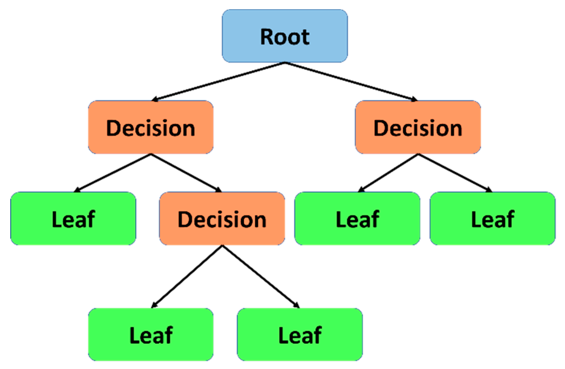
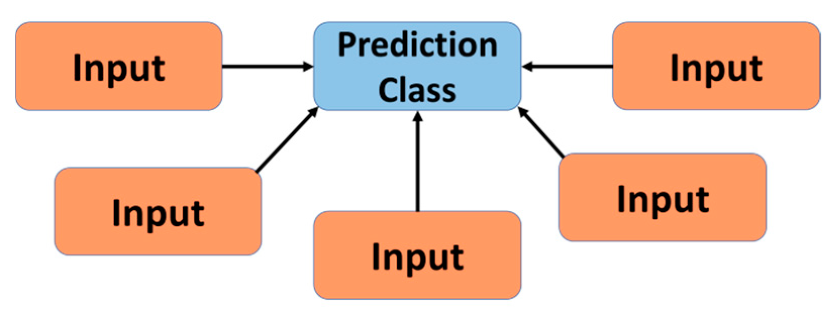
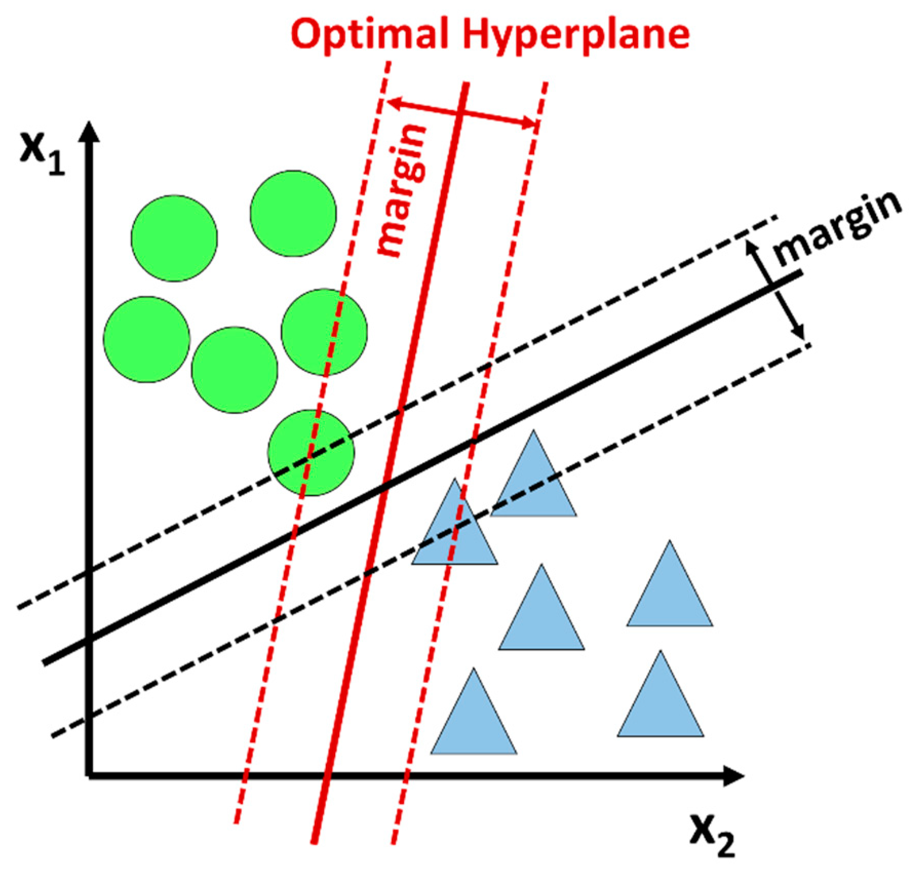
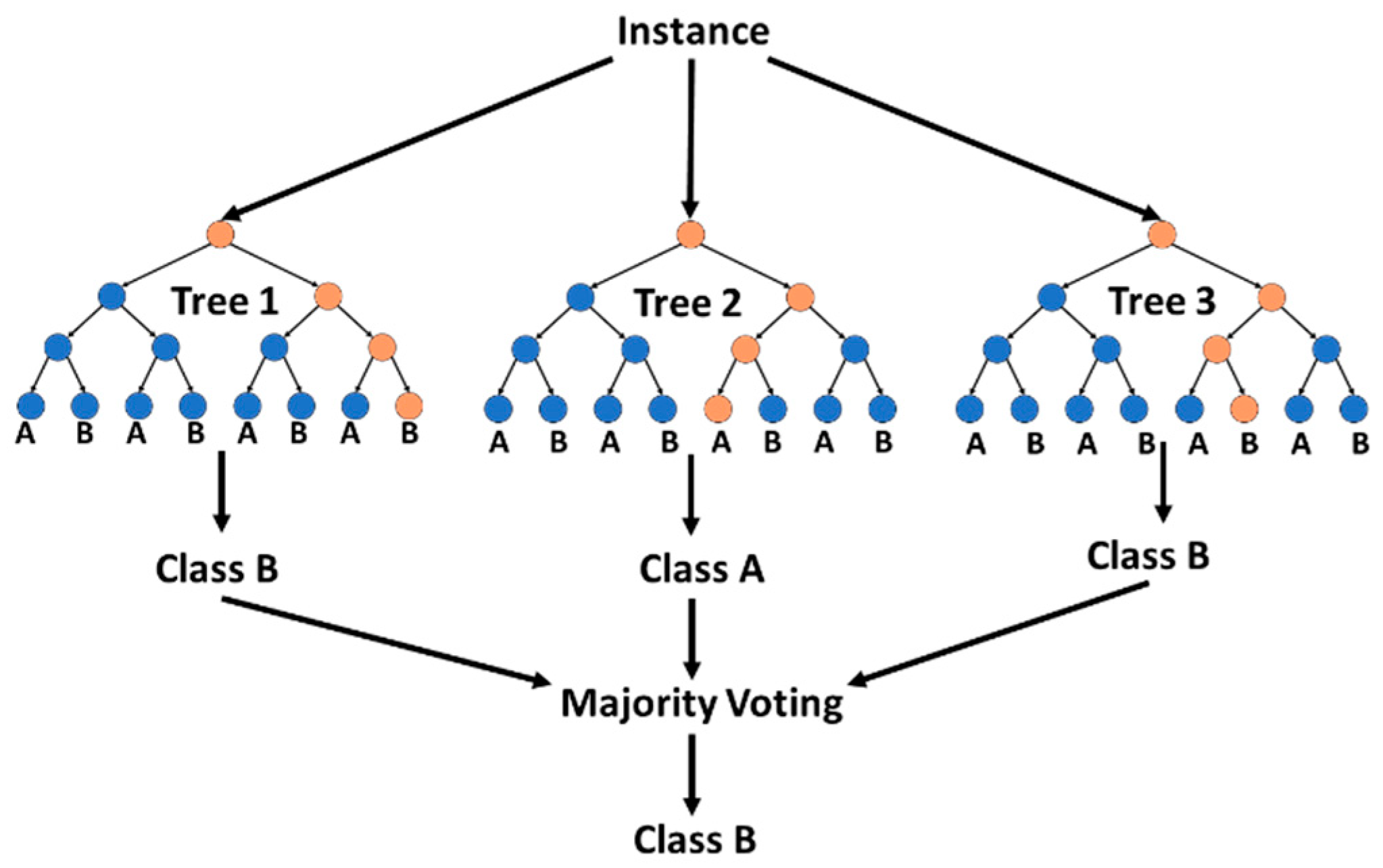
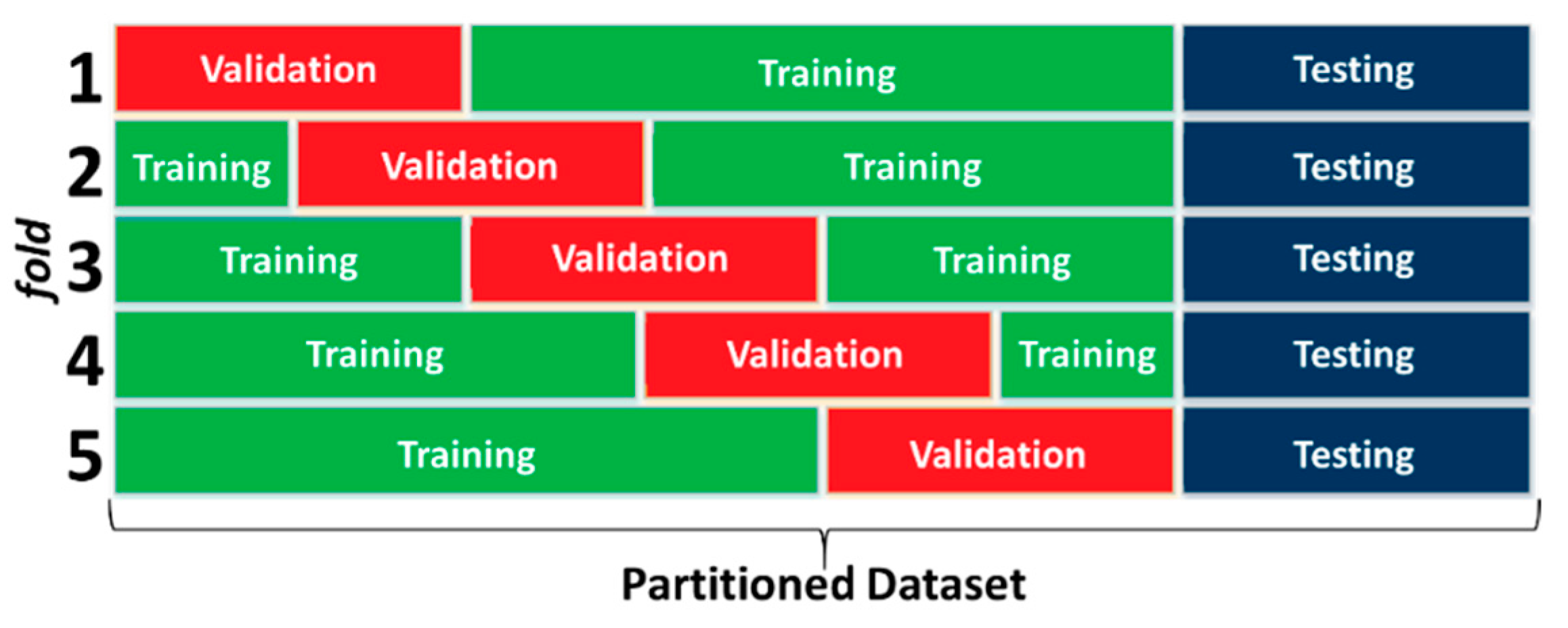
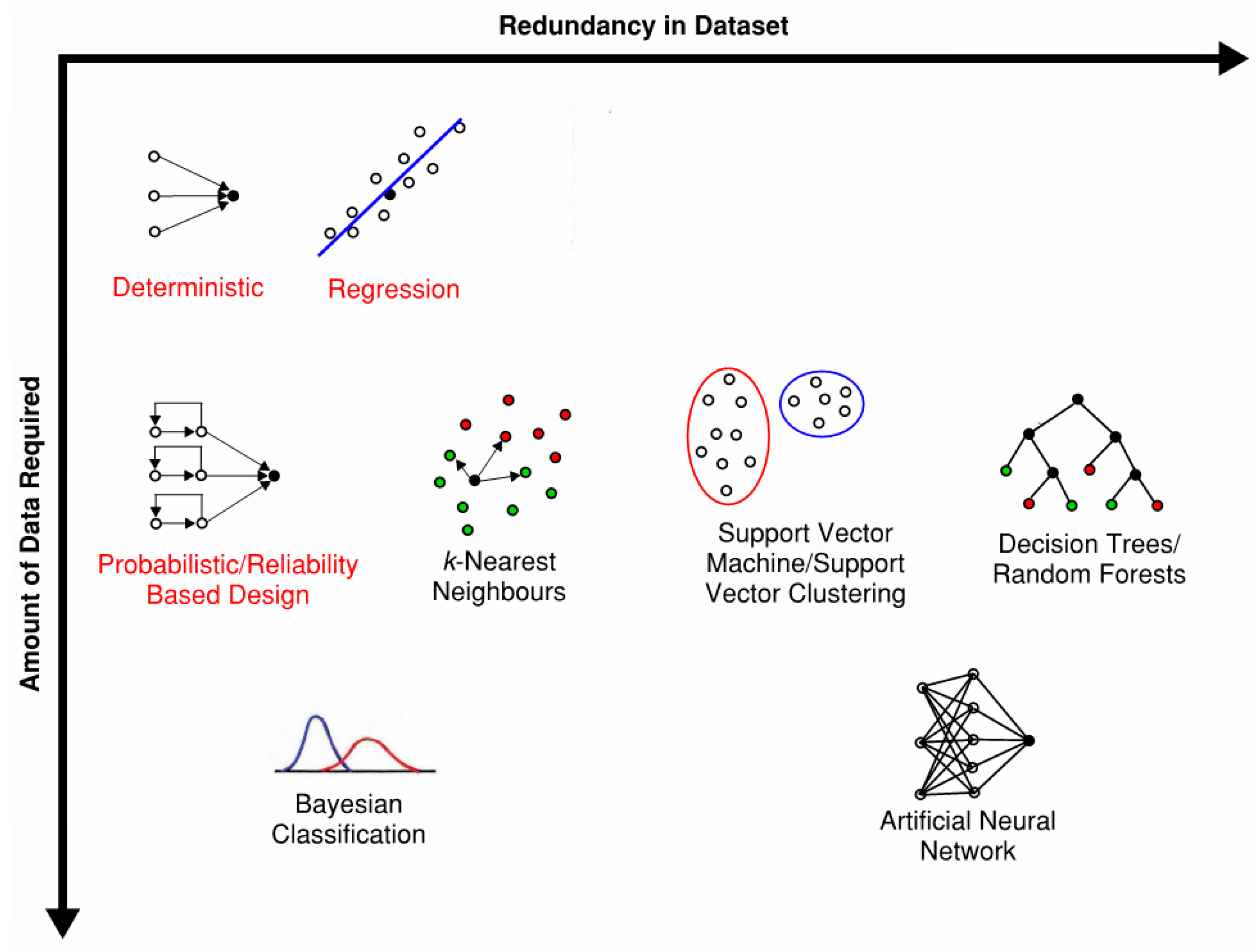
Table 1.
MLAs applied to various rock engineering problems.
| Rock Engineering Problem | MLAs | Opportunities |
|---|---|---|
| Rock mass properties | Categorical ANNs [52,83,84] | • Backwards predict rock mass properties based on observed site conditions • Predict rock mass scale properties based on lab-scale properties and rock mass behaviour |
| Laboratory testing and constitutive behaviour | Numerical ANNs [54,85] SVM [85] | • Use geology and peak Unconfined Compressive Strength to predict crack initiation and crack damage thresholds • Use laboratory tests and field observations to predict constitutive behaviour • Use rock mass scale classification (e.g., Q, RMR) to predict lab-scale properties |
| Slope stability | Categorical ANNs [57,86] SVM [87] RF [88,89] Clustering [90] | • Predict slope movements based on geometry, piezometers, inclinometer data, etc. • Predict volume of structurally controlled failure based on mapped discontinuities |
| Point cloud analysis | RF [91] kNN [92] | • Use successive tunnel scans to get volume differences and predict time-dependent deformations |
| Tunnel performance | Numerical ANNs [55,93,94,95] Categorical ANNS [96,97] SVM [69] RF [61,70] | • Predict stress/strain fields for input into numerical models • Use preliminary/incomplete field mapping to prediction rock mass classification (e.g., Q, RMR) • Predict tunnel support class based on rock mass classification (e.g., Q, RMR) • Predict rock support performance-based on geology, excavation method, environmental conditions, etc. • Use microseismic monitoring arrays to predict rock mass deformation as excavation is developed |
| Rock bursts | Categorical ANNs [65] Naïve Bayesian classifiers [65] kNN [65] RF [98] SVM [65,99] Decision Trees [62] | • Predict magnitude and location of events using 3D excavation geometry, time-series seismic events, mapped geology, etc. • Use previous rockburst events, geology, etc. to predict magnitude of failed material and performance of rock support • Use mapped rock classification (e.g., Q, RMR) to predict probability of rockburst |
| Blasting | Categorical ANNs [100,101] Numerical ANNS [100] SVM [99,102] RF [102] | • Use blast parameters and damage extent to predict optimum parameters for future blasts • Predict blast parameters using mapped rock classification (e.g., Q, RMR) |
© 2019 by the authors. Licensee MDPI, Basel, Switzerland. This article is an open access article distributed under the terms and conditions of the Creative Commons Attribution (CC BY) license (http://creativecommons.org/licenses/by/4.0/).
Share and Cite
MDPI and ACS Style
Morgenroth, J.; Khan, U.T.; Perras, M.A. An Overview of Opportunities for Machine Learning Methods in Underground Rock Engineering Design. Geosciences 2019, 9, 504. https://0-doi-org.brum.beds.ac.uk/10.3390/geosciences9120504
AMA Style
Morgenroth J, Khan UT, Perras MA. An Overview of Opportunities for Machine Learning Methods in Underground Rock Engineering Design. Geosciences. 2019; 9(12):504. https://0-doi-org.brum.beds.ac.uk/10.3390/geosciences9120504
Chicago/Turabian StyleMorgenroth, Josephine, Usman T. Khan, and Matthew A. Perras. 2019. "An Overview of Opportunities for Machine Learning Methods in Underground Rock Engineering Design" Geosciences 9, no. 12: 504. https://0-doi-org.brum.beds.ac.uk/10.3390/geosciences9120504
Note that from the first issue of 2016, this journal uses article numbers instead of page numbers. See further details here.