
Temporal Evolution of Vehicle Exhaust Plumes in a Congested Street Canyon Environment

1
Division of Environment and Sustainability, The Hong Kong University of Science and Technology, Hong Kong SAR, China
2
Department of Marine Environment and Engineering, National Sun Yat-Sen University, Kaohsiung 804201, Taiwan
3
School of Geography and Environment, Shandong Normal University, Jinan 250358, China
4
Department of Mechanical Engineering, The University of Hong Kong, Hong Kong SAR, China
*
Author to whom correspondence should be addressed.
Environments 2024, 11(3), 57; https://0-doi-org.brum.beds.ac.uk/10.3390/environments11030057
Submission received: 5 January 2024
/
Revised: 10 March 2024
/
Accepted: 11 March 2024
/
Published: 15 March 2024
(This article belongs to the Special Issue Advances in Urban Air Pollution)
Abstract
:Air pollutants from traffic make an important contribution to human exposure, with pedestrians likely to experience rapid fluctuation and high concentrations on the pavements of busy streets. This monitoring campaign was on Hennessy Road in Hong Kong, a densely populated city with deep canyons, crowded footpaths and low wind speeds. Kerbside NOx concentrations were measured using electrochemical sensors with baseline correction and subsequently deconvoluted to determine concentrations at 1-s resolution to study the dispersion of exhaust gases within the first few metres of their on-road source. The pulses of NOx from passing vehicles were treated as segments of a Gaussian plume originating at the tailpipe. The concentration profiles in segments were fit to a simple analytical equation assuming a continuous line source with R2 > 0.92. Least squares fitting parameters could be attributed to vehicle speed and source strength, dispersion, and sensor position. The width of the plume was proportional to the inverse of vehicle speed. The source strength of NOx from passing vehicles could be interpreted in terms of individual emissions, with a median value of approximately 0.18 g/s, but this was sensitive to vehicle speed and exhaust pipe position. The current study improves understanding of rapid changes in pollutant concentration in the kerbside environment and suggests opportunities to establish the contribution from traffic flow to pedestrian exposure in a dynamic heavily occupied urban microenvironment.
1. Introduction
The roadsides of busy urban streets are polluted environments [1,2]. The traffic emissions pose adverse public health impacts, including respiratory health problems and allergies; pedestrians, drivers and residents in nearby naturally ventilated buildings are among those affected [3,4,5]. Concentrations of traffic-derived pollutants are especially high in urban street canyons [6,7,8,9,10,11], where elements of the roadside architecture [12] such as bus stops [13,14], overhead walkways [15], and roadside vegetation [16,17,18] can inhibit airflow. Vehicles induce turbulence and canyon winds along the canyon axis [19,20]. Automotive exhaust plumes, especially during congestion and queuing [21,22], lead to high concentrations and chemical reactions that cause rapid variation in street-level air pollutants in this dynamic environment, with the potential for rapid ozonolysis of nitric oxide (NO) to nitrogen dioxide (NO2) [19,23]. Furthermore, nucleation, condensation, secondary particle production, and adsorption of pollutants onto the aerosol are likely to be important [24]. Such processes could also produce varying amounts of nanoparticles and reactive oxygen species [25] and induce their variability in urban air [26].
Urban streets are important communal spaces for outdoor activities where pedestrians on pavements may be just a few metres from traffic; near-field pollutants represent a major source of human exposure, which is poorly represented by fixed monitoring sites located away from the kerbside [27,28]. Such pollution has been investigated using portable sensor measurements on the roadside [19] or from vehicles [29,30], which have been useful in assessing vehicle emissions [6,31]. The dispersion of exhaust gases in the first few metres is complex [32,33], where emissions are affected by turbulent vehicle wakes [34] and mix into the lower street canyon [19].
Hong Kong, the site of this study, is a densely populated city. The suburb of Kwun Tong supports 57,250 persons per square kilometers [34], which is among the most crowded districts in the world. The city is characterized by a vertical environment with over 500 habitable high-rise buildings that have over 40 floors, creating deep street canyons. In Hong Kong, vehicles are a significant source of air pollution, with nearly 20% of NOx and 50% of carbon monoxide (CO) emissions originating from the transport sector ranked as the third highest source of NOx and the highest source of CO according to Hong Kong Air Pollutant Emission Inventory [35]. Buses and trucks are particularly important contributors as private vehicle ownership is relatively low in Hong Kong. Diesel buses play a vital role in the daily lives of residents, with only 573,571 private vehicles registered in January 2020, or about 7600 per 100,000 people [36]. The kerbside environment is subject to high concentrations of pollutants. However, Hong Kong has only three roadside stations, and these are often elevated above pedestrians. These roadside sites average at [37]: NOx 105 ± 25, NO2 44 ± 3.2, and CO 698 ± 50 ppb (years 2017/2019 to avoid COVID-19 years). The urban footpaths are heavily used in Hong Kong, crowded with people waiting for buses and trams, merchants. Domestic helpers who act as live-in maids frequently occupy these spaces to socialize on Sundays [38]. This highlights the importance of understanding and managing air quality in such densely populated environments.
Vehicle exhaust gas dispersion behavior has been investigated through various methods. Computational fluid dynamics (CFD) models have been employed to simulate exhaust gas dispersion from vehicle exhaust pipes [39,40,41,42]. Studies [43,44,45,46] have examined the effects of initial emission concentration, exit velocity, exit direction, and crosswind intensity on exhaust plume dispersion, both experimentally and numerically. CFD studies of street canyons have offered valuable insights into wind fields and pollutant transport [47,48], The results indicate that street geometry, such as aspect ratio [49,50], building height [51], and urban forestry [52,53,54], significantly and collectively impacts pollutant distributions in the canyons [55]. These simulations have been validated through comparison with wind tunnel experiments [56,57]. The Large Eddy Simulation (LES) method has proven to be more accurate than Reynolds Averaged Navier Stokes (RANS)-based techniques [58,59]. However, the RANS modeling approach remains popular due to its lower computational cost and time requirements [55,60].
Quantifying the air quality at the roadside is important for regulating air pollution and assessing health impacts; therefore, real-world roadside monitoring has been conducted. The concentration gradients within this heterogeneous environment were found to be steep [29], so it can be hard to estimate pedestrian exposure [28]. Moreover, the majority of studies have focused on experiments in relatively ideal microenvironments, such as wind tunnels [57] and controlled lab-like environments [43,44,45]. There is a scarcity of research addressing real-world kerbside measurements. While CFD, LES, and other sophisticated numerical models offer valuable insights into the vehicle plume dispersion process in the near-wake region, their massive computational cost and slow rate of calculation limit their real-time applicability in city-scale implementations [61]. Therefore, there is a need for more practical approaches to study and manage air quality in real-world urban environments. Gaussian models are commonly used to simulate atmospheric pollutant dispersion near sources as they provide an efficient compromise between reasonable accuracy and manageable computational time [62]. In a previous study, a modified Gaussian model was utilized to simulate NOx concentrations in a comprehensive case study [62].
The study described here deployed multiple high-time resolution sensors (1-s) near a congested lane of traffic for NOx. The sensors respond rapidly to changes in pollutant concentration after deconvolution algorithm correction. A modified classical Gaussian dispersion model was employed to describe the concentration profiles emitted from individual vehicles. While a Gaussian model may not be a proper formulation in this near-source turbulent environment (Reynolds numbers 105 to 108) [63], it offers a reasonable choice as a fitting equation. Hence, the structure of the NOx plumes has been fitted to assess dispersion parameters and the source strength of passing vehicles. It also attempts to relate these to emissions as determined from the NOx: CO2 ratio in exhaust plumes. Such estimates can be especially important for roadside NOx as standards have typically been difficult to meet in Hong Kong [64]. We specifically selected NOx as the target pollutant due to its identification as the primary challenge for improving air quality in Hong Kong [65]. The results provide an indication of the rapid changes in kerbside pollutant concentrations, propose a new method for modelling vehicle emissions in the roadside environment, and aid understanding of pedestrian exposure, but the relevance of short high-concentration cumulative exposure needs to be better understood [66].
2. Methodology
2.1. Instrumentation
The high-speed sensors (HSS-100, Sapiens, Shen Zhen, China) used at this site have been described in earlier work [6]. In brief, the devices actively sample air to determine concentrations of NO, NO2, and CO2 using 4-electrode electrochemical sensors (Table 1) with proprietary baseline sensors incorporating pair differential filter (PDF) technology to reduce the baseline drift due to humidity and temperature changes [67]. The 1-s resolution captures the rapidly changing pollutant concentrations in the plume segments. Real-time sensor data is processed with an on-board microprocessor and transferred to a local server by a Wi-Fi module.
2.2. Site
This study examines a site on Hennessy Road, Causeway Bay, Hong Kong (22°16′48.0″ N 114°10′57.9″ E), an area with a population density of about 17,000 inhabitants per square kilometre. Known for its shopping malls and significant commercial foot traffic, the area has heavily occupied pavements, making it an important location for studying air quality and pollution in an urban setting. The road lies in a deep urban canyon with walls of 20–40 floors (~120–220 m; in our site, the aspect ratio is ~3.9 to 2.6) and low wind speeds; median and Q3 were 0.6 and 1.2 m·s−1 at node R2, respectively [19]. Heavy vehicles are a focus of emission reduction in the city, and the site is near one of Hong Kong’s Franchised Bus Low Emission Zones, where the Euro V standard is required for buses [68]. Kerbside measurements on Hennessy Road were made between 09:00 and 21:00 on four working days during December 2020, i.e., 21 December, 22 December, 28 December, and 29 December. The site is on a dual carriageway, with one side lined with tall buildings and the other featuring an electric tram stop and footbridge stairs. This relatively confined space limits the influence of opposing traffic lanes. Figure 1 illustrates the location of the canyon sampling site.
Seven high-speed sensors were deployed at the site (detailed in [19]). Four (L1, L2, R1, and R2) were positioned on both sides of the lane to capture as many of the exhaust plumes as possible, regardless of the direction of dispersion through turbulence or local winds (Figure 1c). Wind speed and direction were measured with a wind sensor (HY-WDC5, Hongyue, China) at L2 and R2. Sensor inlets L1, L2, R1, and R2 were close to the height of tailpipes for buses (0.4–0.6 m), which are the dominant pollutant source at the site. Others were deployed in more elevated positions; one on a lamp post (LH) at 1.6 m measured the concentration of the breathing zone. The left lane was blocked during the monitoring campaign (Figure 1e), so traffic gradually moved to the right and tended to flow along the lane closest to nodes R1 and R2. However, the transverse position of the exhaust plumes varies depending on the bus model. Pollutant fluctuations have been presented in the previous study [19].
The calibration and QA/QC for the monitoring system Is described in earlier work [6,67]; more details can be found in the Supplementary Materials. Nitrogen oxides were generated with a NO2/NO/O3 calibration source (Model 714, 2B Technology, Boulder, CO, USA). Time synchronization was important when comparing sensors and pair plumes with passing vehicles, so the internal clocks at each sampling node were synchronized every day before the deployment and every four hours during the campaigns.
Number plate recognition enabled individual vehicles to bed and matched to emission factors (EFs). This used a road-side camera to image the number plates, which could then be compared to non-private registration information, including engine size, vehicle type, fuel consumption, and registration year. Emission factors take a range of units: mass of pollutant per unit time, distance travelled, or engine output, while others are mass of pollutant per mass of fuel. As field measurements do not sample directly from exhaust plumes, they often allow for dilution using mass-based EFs (g kg−1), adjusted by measuring CO2 concentration at the same time as the target pollutant. The EFs used in this study were determined as a differential with respect to CO2 concentration across the plume segments as described by [6]. In the current work, vehicle emissions were additionally expressed as a source strength g s−1, but with knowledge of vehicle fuel consumption and speed, it can be related to EFs of vehicles specified through number plate recognition.
2.3. Plume Segment Description
CFD is a successful and popular approach to describing vehicle exhaust plumes [10,21,32,69]. However, it is computationally expensive and remains sensitive to dispersion, so it is best suited to stable atmospheric conditions [70]. In this study, we chose a simple analytical equation to describe dispersion of the vehicle exhaust pollutants by adopting the classical Gaussian equation for a continuous point source [71]. This equation is commonly used in air pollution modeling to estimate the concentration of pollutants at a given distance from a source. The pollutant dispersion is described using a Gaussian model, where the concentration decreases as the distance from the source increases [72]. By using this equation, we estimated the concentration of pollutants at different distances from the source (i.e., different times after a vehicle has passed) without needing complex parameterization and computationally expensive CFD simulations.
Cx,y,z = Qp/(2πuσyσz) exp(−y2/2σy2) [exp(−(−H)2/2σz2) + exp(−(z + H)2/2σz2)]
- Cx,y,z (g m−3)—concentrations in a plume at location (x, y, z)
- y (m)—the distance of the sensor from the vehicle exhaust in crosswind direction
- z (m)—the distance of the sensor from the vehicle exhaust in vertical direction
- H (m)—elevation height from the ground
- σz, σy—the pollutants advect with the wind and disperse vertically (z-direction) and crosswind-wise (y-direction)
- u (m/s)—windspeed
- Qp (g s−1)—source strength
In the case of a vehicle plume where concentrations are measured at roadside sensors in a stagnant canyon, a different frame of reference is employed. Unlike the plume from a chimney as a source, the vehicle is moving along the road, with the sampling site stationary. Thus, the kerbside monitors cut a segment through the expanding plume, so when the equation is considered from the reference frame of the source, the windspeed (u) becomes the velocity of the vehicle (v). This means that the sensors sample the emissions generated at a single instant, so changes are due to the expansion and dispersion of the pollutants. It is idealized, but it describes a form that can fit the data with parameters that offer the potential of physical interpretation.
In the aerodynamic environment of a busy road, we have made a number of assumptions: (i) z = H = 0, as the sensors’ inlets were at the same height of the tailpipe, so the terms within the square brackets become 2; and (ii) the dispersion in the turbulent vehicle wake are equal along both y- and z-axes (i.e., σ = σy = σz). The equation is simplified to give the concentration at the monitoring site Cs:
where ys is the distance of the sensor from the vehicle exhaust. Turbulence in the vehicle wake will mean that the initial dispersion will likely have a dimension of one to a few metres [32], which will affect agreement with the equation close to the origin of the plume. Subsequently, plume spread (a) is a function of distance travelled by the vehicle, i.e., σ ~ axn, but a plume from a tailpipe is typically thin [70] and likely to spread almost linearly with distance, such that σ = ax and x is the distance that the vehicle has travelled. However, for our measurements, this distance may be related to time from the velocity (v) of the passing vehicles:
after adding the local background concentration, Cb. Note the very strong dependence on vehicular velocity (1/v3) in the trailing part of the plume. The presence of a crosswind would mean that y would vary over time, but under low windspeeds typical of the canyon [19], this would be linear with time and incorporated within parameter a. We have, for simplicity, neglected dispersion along the plume axis (σx), although this could be important in such a turbulent environment close to the source [73].
Cs = Qp/(πvσ2) exp(−ys2/2σ2)
Cs = Cb + Qp/(πa2v3t2) exp(−ys2/2a2v2t2)
2.4. Data Analysis and Deconvolution
A least squares approach allowed the parameters X1, X2, and X3 in the non-linear equation developed from Equations (2) and (3) to be solved from:
Cs = X1 + (X2/t2) exp(−X3/t2)
This describes the plume segments characteristically seen in the monitoring record from the kerb [6]. The nonlinear equation (Equation (4)) was fit using a least squares routine from the scipy library (version 1.9.1) in Python (version 3.9.13) [74]. Figure 2a shows a typical fit to a plume segment extracted from the monitoring record (inset to Figure 2a). The segment has a steep leading edge as the sensor encounters the dispersing pollutants, followed by a slower inverse-square law decrease in concentrations as the plume expands and the segment tail passes by the sensor. The fitting parameters extracted typically explained >95% of the variance.
Pollutant sensors are recognised as having slow response times [67], which poses challenges when examining plumes with rapidly changing concentrations. Although the fitting results in our study appeared satisfactory (R2 > 0.92), we observed evidence of systematic errors. Specifically, the fitted concentrations were underestimated in the initial stages of the plume’s trailing part and overestimated towards the end of the measurements (Figure 2a). This suggested it would be important to enhance the temporal resolution of the measurements, processing the signal to reduce the effects of sensor response. Fourier deconvolution, the inverse of Fourier convolution, has been utilized to improve the response time of low-cost sensors [75]. In signal processing, it can be employed as a computational method to reverse the result of a convolution occurring in the physical domain. In this study, we assume the slow sensor response output is the result of a convolution occurring in the physical domain [76]. Therefore, deconvolution was used to reverse the signal distortion caused by the sensors and reconstruct the original rapidly changing signal [59].
We determined the sensor response from laboratory measurements of a step-like change in pollutant concentrations as shown in Figure 2b (using the setup described in [67]). This formed the exponential kernel as shown in Figure 2c (trial and error optimised this to 11 points 0–10 s of e−0.2t), which allowed these laboratory output signals to be deconvoluted (Figure 2b). The error of deconvolution has been visualized in the Supplementary Materials (Figure S2). This kernel, of the same form as that used by [75], was used in the deconvolution routine fft of the numpy library in Python [74].
The concept of convolution and deconvolution clearly explains the characteristics of fits (Figure 2d), where we can see the plume structure of an idealised plume (effectively deconvoluted data) represented by the red + and the fitted curve as well as data convoluted (black +) with the kernel (i.e., ‘raw measurements’). The raw measurements are fitted according to Equation (4) with a black line and show the systematic error described previously, i.e., the fitted curve is low at the beginning of the trailing edge and high at the end, with a peak that arrives early. The deconvolution of real-world measured field data is shown in Figure 2e. When the concentration measurements are deconvoluted, the noise is enhanced, as is typical during deconvolution [76], but when fitted to Equation (4), it takes the expected form as most of the value will not be affected after deconvolution. Deconvolution tends to overemphasise the peak values, but we have used the fitting parameters (X) throughout the paper as they are less sensitive to induced noise.
2.5. Statistical Analysis
The distribution of pollutant concentrations and EFs were often highly skewed, so in addition to means and standard deviations, we used medians and lower and upper quartiles (Q1 and Q3) to describe the central tendency and statistical dispersion. The Kendall rank correlation (statistic τ) was sometimes chosen in preference to the more common Pearson R2 as it is robust against outliers or non-normal distributions. Cross-correlation used the online calculator available from WessaNet [77].
3. Results
3.1. Evaluating Plume Parameters and Deconvolution
The aforementioned model had three unknown parameters: X1, X2, and X3, representing Cb, Qp/πa2v3 and ys2/2a2v2, respectively. Note that ys is assumed to be constant throughout all the measurements, though it depends on the position of the vehicle exhaust, alignment of the vehicle path along the road, and wind direction. Other parameters might not be constant even across a single plume segment, so the turbulence and plume spread might change the value a; moreover, v can vary as vehicles often accelerate along this section of road. The values of X1, X2, and X3 were extracted from 100 well-defined bell-like plumes and appear after a vehicle passes within 8 s segments for NOx; they are summarised in Table 2 along with fits for the deconvoluted data that improved the time resolution of the measurements. Concentration measurements from plumes were also fit to the parameters after deconvoluting to increase the time resolution of concentrations (as previously shown in Figure 2e). The units are in mass here as that is convenient when considering the source and source strength, though our concentrations were ppb (i.e., a mixing fraction), so we had to convert units at various points and, for simplicity, adopted NO: 1 ppb = 1.25, NO2: 1 ppb = 1.88 μg m−3, with NOx treated as 1 ppb = 1.88 μg m−3, following the usual convention.
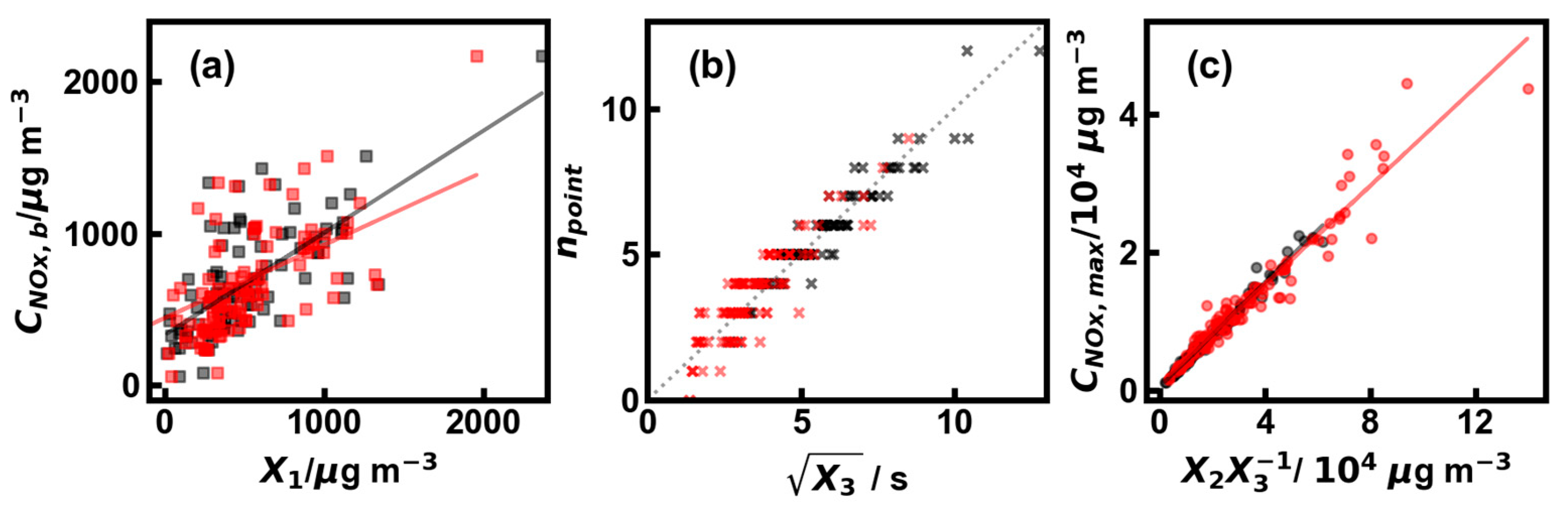
The values of the three parameters X1, X2, and X3 are related to physical aspects of the plume segments as illustrated in Figure 3. These parameters were also evaluated after deconvolution: X1,d, X2,d, and X3,d. As expected, the value X1 is strongly related to the background NOx concentrations, so Figure 3a shows (black points) that it approximates the background concentration, defined as the lowest concentrations just before the start of the plume, though X1 is sometimes slightly negative when extracting the best fit (Figure 3a). It has a median value of 442 μg m−3, which is close to the median value of the baseline (CNOx,b) at 601 μg m−3. The deconvoluted data gives a scattered agreement with the background correlation, with a median value of 438 μg m−3.
The derivative of Equation (4) is 2X2(X3 − t2) exp(−X3/t2)/t5, which becomes 0 when t2 = X3 (i.e., the peak point concentration as shown in Figure 2). This relationship is borne out in Figure 3b, where it can be seen that the number of 1-s observations before the maxima is closely related (τ = 0.86; p < 0.0001) to the square root of X3. The dotted 1:1 line is set through the origin, although no points occur at zero. The deconvoluted parameter X3,d (red) is smaller compared with that derived from the original data because the deconvoluted peak had decreased lag and naturally occurs earlier in the timeline. Peak point concentration can be solved as (X2/X3) exp (−1) when t2 = X3. As shown in Figure 3c, the maximum concentrations measured in the plume segments are a function of X2/X3. The slope of the line is 0.379 ± 0.005 for raw data and 0.358 ± 0.009 for the deconvoluted data. These values are almost identical to those that were expected, i.e., exp (−1), or 0.3679 in this case.
The effectiveness of the deconvolution was validated by applying the kernel to idealised plume segments and revealed that raw data could be effectively deconvoluted to close the initial signal, as illustrated in an idealised case in Figure 2c. Deconvolution removed sensor lag, so the peak concentrations occurred earlier (Figure 3b; Table 2). However, the fitted background concentrations showed more noise in the deconvoluted data because the deconvoluted background fluctuated. It is also important to note that we assumed that the NO2 and NO deconvolution kernels were the same, though the NO2 is likely to be slower (see Table 2). This could introduce some error in the deconvoluted estimates at the end of the trailing edge where NO2 is elevated as the air mixed in the plume, but as NO2 concentrations are low in the near-wake area [19], this source of error is negligible. Despite this limitation, our analysis focused primarily on plume segments, rendering this issue inconsequential for our study.
3.2. Dispersive Parameters within Plume Segments
The term a in Equation (3) relates to the dispersion characteristics of the plume as it spreads over distance or time. If a vehicle were moving rapidly, the plume would stretch out and become narrow. This is supported (τ = 0.74; p < 0.0001; τd = 0.71; pd < 0.0001) by Figure 4 where a is plotted as a function of inverse velocity (1/v). The median value of a is 0.0199 and ~0.0342 for the deconvoluted data, suggesting a slender plume that is much narrower than the elevated plumes described by [71,72]. Our estimates mean that after 10 s at 30 km h−1, these vehicle exhaust plumes would have a width of just 4.5 m. The low values of parameter a estimated here may also have been biased because we chose very clear and well-defined plume segments for analysis. Nevertheless, the observations of [21] suggest exhaust plumes maintain their position behind vehicles over several metres, and σy seems about ¼ the vehicle width at that point. They noticed that heated gases from the exhaust pipe were trapped in the recirculation zone just downstream of the vehicle and that the plume is quite narrow over a number of vehicle lengths.
3.3. Plume Segments at Different Nodes
As multiple sensors were deployed at the site, the plume segments from passing vehicles can be seen in raw data from different sensors (Figure 5a). The positions of the sensors on different sides of the road, along its length, or at elevation mean that the signal arrives at different times, as can be shown by cross-correlation analysis [19]. The three box and whisker plots on the left of Figure 5b show the time differences for raw data from the plumes compared with sensor L2. The plume arrived earlier at R2 as the trajectory of most vehicles took a path towards that sensor, but it arrived later at LH. The time differences (Figure 5a) from cross-correlation analysis compared to sensor L2 reveals similar lags to those found from the arrival time of concentration peaks at different sensors (right-hand box and whisker plots in Figure 5b). These displacements indicate that these are plumes from the same vehicles and are displaced by the arrival time of the pollution segment at the different sensors.
Figure 5c shows the displacement times of the maximum concentration between raw data collected at sensors L1 and L2 as a function of mean wind speed during the plume period. It shows that higher speeds mean fewer differences in the time between the sensors capturing the peak (τ = −0.32; p < 0.01). The fitting parameter X2, estimated from the same plume segment caught on different sensors (L2 and LH: Figure 5d) at the same point on the road, though at different heights, should be similar. This is because the plume segments derive from the same vehicle at a similar time, so they relate to a common source strength (Qp). Figure 5d shows that parameters X2,LH and X2,L2 are highly correlated, with a slope close to unity (slope: 0.90 R2: 0.76 for convoluted data and slope 0.89, R2: 0.88 for deconvoluted data), suggesting that these truly derive from the same plume segment. This agreement adds support to the simple Gaussian approach adopted here.
3.4. Estimates for Vehicular Emissions from Plume Segments
The quotient X2/X3 can be expressed as 2Qp/πvys2, which provides direct access to individual vehicle emissions. This is dependent on the distance from the sensor to the tailpipe ys, which was not measured for each passing vehicle in this study. The EF values of each vehicle were determined in an earlier study from NOx:CO2 ratios across plume segments [6]. These can be converted to an emission rate, taking the fuel consumption of different vehicle types [78] and the measured speeds as vehicles passed the sensor. The relationship between Qp estimated from plume parameters and that from NOx:CO2 ratios [6] is shown in Figure 6 for estimates from both the raw and deconvoluted data. This shows the expected relationship, although the correlation is not especially good (τ = 0.26; p < 0.05; τd = 0.28; pd < 0.05). It is evident that the introduction of the deconvolution reprocessing has increased the uncertainty in estimating the emissions. However, the assumptions that windspeed is low and the direction is constant, along with those about fuel consumption, distance to the exhaust (ys), and vehicle speed (v) determined during acceleration, limit the precision of our estimates. The source strength estimated from the plume segments are larger than those determined from the NOx:CO2 ratios, so there may be a systematic error in one of the parameters (i.e., v or ys).
Despite the rather poor correlation, the emissions are in reasonable agreement with expectations. The median Qp,d estimated in the plume segments examined in this study is about 0.18 g s−1 (Q1 = 0.09, Q3 = 0.25), which lies in a similar range to the measurements of [79] made for diesel buses in Zhenjiang, China (~0.19 g s−1, Euro IV buses of [80] ~0.068 g s−1 under steady driving conditions at 30 km h−1 or ~0.06 g s−1 for real-world 25-tonne Euro V vehicles [81]). The emission rates observed in this study are typically from accelerating vehicles, exceeding the Euro V standard required in Hong Kong’s low-emission zones, which would be met with an emission of ~0.13 g s−1 for an engine rated at 243 kW.
Although direct and accurate measurement of emissions from individual vehicles [82] is possible with onboard Portable Emissions Measurement Systems (PEMS), these cannot readily capture larger fleets observable by roadside sensors. Examining a large number of vehicles is useful because the EFs of individual vehicles can vary widely, which is certainly a problem with the Hong Kong fleet [83,84]. However, roadside measurements reflect a local character that may not be representative of the urban fleet in general [6]. Plumes selected in this study captured at our site in Hennessy Road arise mostly from buses and heavy vehicles, which were typically (~70%) accelerating. This means the roadside measurements made here may reveal values of Qp and thus of EF that are high compared with cruise mode. Estimates of EFs using NOx:CO2 ratios, unlike estimates from the plume equation (Equation (3)), have considerable advantages because they allow for dilution so effectively. Nevertheless, it is worth pursuing the plume analysis of the type undertaken in this study as it is not dependent on CO2, which can be difficult to measure in situations where it deviates little from a high background.
4. Conclusions and Discussion
This study adopted a modified Gaussian approach to assessing the structure of NOx concentration profiles captured by a kerbside stationary sensor from passing vehicles in a street canyon, after refinement by deconvolution. The study has enhanced our understanding of real-world plumes measured by the roadside in a comprehensible manner. Even though the vehicle wakes induce turbulence, the concentration profiles were often quite smooth, so there was a good least-squares fit to a simple Gaussian model of the plume segments. Physical features such as the timing and magnitude of the peak in NOx concentrations were realistically expressed by the fitted parameters. Overall, the emission strength of passing buses suggests that they meet the Euro IV standards, and at times, the Euro V standards desired in Hong Kong’s low-emission zones.
While acknowledging a certain degree of sacrificed accuracy, the adoption of this model offers a cost-effective approach that will benefit future kerbside air quality monitoring and real-time forecasting endeavors. By simplifying the complex nature of plume dispersion and analyzing the key factors that influence it, this study enables a more accessible way to predict air quality and estimate pedestrian exposure at the roadside. Moreover, by reducing the reliance on expensive analyzers and resource-intensive modeling, this simplified approach can facilitate more widespread air quality forecasting and management by low-cost sensor networks in blocks or cities, ultimately contributing to healthier urban environments. It is important to note that the equation we adopted in this study treats vehicles travelling along a deep stagnant canyon. It is important to recognize that this treatment may need to be revised or adapted when applied in different environments.
Estimates of the emissions from individual vehicle plumes were hampered by the need for accurate measurements of vehicle speed and tailpipe position in this study. However, further work could resolve some of these problems and thus refine the fitted variables. In particular, estimating the distance between the sensor and the tailpipe (ys) for each vehicle as it passes the site should be relatively simple using video, provided that the tailpipe is visible. However, the uncertainty can be quite significant when estimating emissions as we used low-cost sensors. The reconstruction of signals using the deconvolution method improves the performance of sensors but may introduce other complexities. The utilization of fast-response analyzers coupled with duplicate sampling by a pair of analyzers could contribute to reducing uncertainty in the measurements. We are currently extracting EFs for CO2 by this method as the carbon balance approach is not suitable. Further campaigns could examine roadside sites beyond urban canyons. The analysis of plume segments is also of value in understanding the rapid changes in concentrations to which pedestrians are exposed when sensors are set in the breathing zone. The kerbside environment experiences ozonolysis of NO to NO2 and the production of secondary particles and reactive oxygen species. The complexities and importance of this urban micro-environment make it worthy of continued study.
In summary, this study has provided a simple parameterisation of real-world plumes measured at the roadside but may further offer a potential tool for future air quality forecasting and exposure estimation at the kerbside. The simplified model, while sacrificing some accuracy, offers a cost-effective approach that can be easily implemented and extended, paving the way for more comprehensive air pollution management strategies.
Supplementary Materials
The following supporting information can be downloaded at: https://0-www-mdpi-com.brum.beds.ac.uk/article/10.3390/environments11030057/s1, Figure S1: Calibration step of NO; Figure S2: Schematic showing instrument response to a step change of X; Figure S3: Imposed changes in NOx concentration in laboratory experiments (gray dotted line), concentration measurements as gray lines and deconvoluted concentrations as red dots with error bar represent the absolute errors. Table S1: Calibration Concentration Setting; Table S2: Calibration Instrumentation. Reference [85] is cited in the supplementary materials.
Author Contributions
Conceptualization, P.B. and M.-Y.C.; methodology, P.B. and M.-Y.C.; software, M.-Y.C. and P.W.; formal analysis, P.B., M.-Y.C. and P.W.; investigation, M.-Y.C. and P.W.; resources, Z.N.; data curation, M.-Y.C.; writing—original draft preparation, M.-Y.C. and P.B.; writing—review and editing, Z.N. and C.-H.L.; visualization, M.-Y.C.; supervision, P.B. and Z.N.; project administration, Z.N.; funding acquisition, Z.N. All authors have read and agreed to the published version of the manuscript.
Funding
This study was supported by the European Union (EU)—Hong Kong Research and Innovation Cooperation Co-funding Mechanism by the Research Grants Council (RGC) (RGC Ref.: E-HKUST601/19), the Environment and Conservation Fund (ECF Project 21/2021), and the Collaborative Research Fund (CRF) for 2018/19 (RGC Ref No. C7064-18G).
Institutional Review Board Statement
Not applicable.
Informed Consent Statement
Not applicable.
Data Availability Statement
The original contributions presented in the study are included in the article and Supplementary Materials, further inquiries can be directed to the corresponding authors.
Acknowledgments
The authors gratefully acknowledge the HKEPD for their support in this study. The contents of this paper are solely the responsibility of the authors and thus do not necessarily represent the official views of the Hong Kong SAR Government.
Conflicts of Interest
The authors declare no conflicts of interest.
References
- Johansson, C.; Norman, M.; Gidhagen, L. Spatial & Temporal Variations of PM10 and Particle Number Concentrations in Urban Air. Environ. Monit. Assess. 2007, 127, 477–487. [Google Scholar] [CrossRef]
- Pateraki, S.; Manousakas, M.; Bairachtari, K.; Kantarelou, V.; Eleftheriadis, K.; Vasilakos, C.; Assimakopoulos, V.D.; Maggos, T. The Traffic Signature on the Vertical PM Profile: Environmental and Health Risks within an Urban Roadside Environment. Sci. Total Environ. 2019, 646, 448–459. [Google Scholar] [CrossRef] [PubMed]
- Godri, K.J.; Green, D.C.; Fuller, G.W.; Dall’Osto, M.; Beddows, D.C.; Kelly, F.J.; Harrison, R.M.; Mudway, I.S. Particulate Oxidative Burden Associated with Firework Activity. Environ. Sci. Technol. 2010, 44, 8295–8301. [Google Scholar] [CrossRef] [PubMed]
- Wu, X.; Vu, T.V.; Harrison, R.M.; Yan, J.; Hu, X.; Cui, Y.; Shi, A.; Liu, X.; Shen, Y.; Zhang, G.; et al. Long-Term Characterization of Roadside Air Pollutants in Urban Beijing and Associated Public Health Implications. Environ. Res. 2022, 212, 113277. [Google Scholar] [CrossRef] [PubMed]
- Ai, Z.T.; Mak, C.M. From Street Canyon Microclimate to Indoor Environmental Quality in Naturally Ventilated Urban Buildings: Issues and Possibilities for Improvement. Build. Environ. 2015, 94, 489–503. [Google Scholar] [CrossRef] [PubMed]
- Chu, M.; Brimblecombe, P.; Wei, P.; Liu, C.H.; Du, X.; Sun, Y.; Yam, Y.S.; Ning, Z. Kerbside NOx and CO Concentrations and Emission Factors of Vehicles on a Busy Road. Atmos. Environ. 2022, 271, 118878. [Google Scholar] [CrossRef]
- Krecl, P.; Targino, A.C.; Landi, T.P.; Ketzel, M. Determination of Black Carbon, PM2.5, Particle Number and NOx Emission Factors from Roadside Measurements and Their Implications for Emission Inventory Development. Atmos. Environ. 2018, 186, 229–240. [Google Scholar] [CrossRef]
- Voordeckers, D.; Lauriks, T.; Denys, S.; Billen, P.; Tytgat, T.; Van Acker, M. Guidelines for Passive Control of Traffic-Related Air Pollution in Street Canyons: An Overview for Urban Planning. Landsc. Urban Plan. 2021, 207, 103980. [Google Scholar] [CrossRef]
- Voordeckers, D.; Meysman, F.J.R.; Billen, P.; Tytgat, T.; Van Acker, M. The Impact of Street Canyon Morphology and Traffic Volume on NO2 Values in the Street Canyons of Antwerp. Build. Environ. 2021, 197, 107825. [Google Scholar] [CrossRef]
- Westerdahl, D.; Wang, X.; Pan, X.; Zhang, K.M. Characterization of On-Road Vehicle Emission Factors and Microenvironmental Air Quality in Beijing, China. Atmos. Environ. 2009, 43, 697–705. [Google Scholar] [CrossRef]
- Wang, H.; Brimblecombe, P.; Ngan, K. A Numerical Study of Local Traffic Volume and Air Quality within Urban Street Canyons. Sci. Total Environ. 2021, 791, 148138. [Google Scholar] [CrossRef] [PubMed]
- Vardoulakis, S.; Fisher, B.E.A.; Pericleous, K.; Gonzalez-Flesca, N. Modelling Air Quality in Street Canyons: A Review. Atmos. Environ. 2003, 37, 155–182. [Google Scholar] [CrossRef]
- Xing, Y.; Brimblecombe, P.; Ning, Z. Fine-Scale Spatial Structure of Air Pollutant Concentrations along Bus Routes. Sci. Total Environ. 2019, 658, 1–7. [Google Scholar] [CrossRef] [PubMed]
- Yang, F.; Kaul, D.; Wong, K.C.; Westerdahl, D.; Sun, L.; Ho, K.; Tian, L.; Brimblecombe, P.; Ning, Z. Heterogeneity of Passenger Exposure to Air Pollutants in Public Transport Microenvironments. Atmos. Environ. 2015, 109, 42–51. [Google Scholar] [CrossRef]
- Duan, G.; Brimblecombe, P.; Chu, Y.L.; Ngan, K. Turbulent Flow and Dispersion inside and around Elevated Walkways. Build. Environ. 2020, 173, 106711. [Google Scholar] [CrossRef]
- Abhijith, K.V.; Kumar, P. Field Investigations for Evaluating Green Infrastructure Effects on Air Quality in Open-Road Conditions. Atmos. Environ. 2019, 201, 132–147. [Google Scholar] [CrossRef]
- Buccolieri, R.; Jeanjean, A.P.R.; Gatto, E.; Leigh, R.J. The Impact of Trees on Street Ventilation, NOx and PM2.5 Concentrations across Heights in Marylebone Rd Street Canyon, Central London. Sustain. Cities Soc. 2018, 41, 227–241. [Google Scholar] [CrossRef]
- Kumar, P.; Zavala-Reyes, J.C.; Tomson, M.; Kalaiarasan, G. Understanding the Effects of Roadside Hedges on the Horizontal and Vertical Distributions of Air Pollutants in Street Canyons. Environ. Int. 2022, 158, 106883. [Google Scholar] [CrossRef]
- Brimblecombe, P.; Chu, M.Y.; Liu, C.H.; Ning, Z. NOx and CO Fluctuations in a Busy Street Canyon. Environments 2021, 8, 137. [Google Scholar] [CrossRef]
- Zhao, Y.; Jiang, C.; Song, X. Numerical Evaluation of Turbulence Induced by Wind and Traffic, and Its Impact on Pollutant Dispersion in Street Canyons. Sustain. Cities Soc. 2021, 74, 103142. [Google Scholar] [CrossRef]
- Gosse, K.; Gonzalez, M.; Paranthoën, P. Mixing in the Three-Dimensional Wake of an Experimental Modelled Vehicle. Environ. Fluid Mech. 2011, 11, 573–589. [Google Scholar] [CrossRef]
- Lin, J.; Ge, Y.E. Impacts of Traffic Heterogeneity on Roadside Air Pollution Concentration. Transp. Res. D Transp. Environ. 2006, 11, 166–170. [Google Scholar] [CrossRef]
- Zhang, K.; Chen, G.; Zhang, Y.; Liu, S.; Wang, X.; Wang, B.; Hang, J. Integrated Impacts of Turbulent Mixing and NOX-O3 Photochemistry on Reactive Pollutant Dispersion and Intake Fraction in Shallow and Deep Street Canyons. Sci. Total Environ. 2020, 712, 135553. [Google Scholar] [CrossRef]
- Olivares, G.; Johansson, C.; Ström, J.; Hansson, H.-C. The Role of Ambient Temperature for Particle Number Concentrations in a Street Canyon. Atmos. Environ. 2007, 41, 2145–2155. [Google Scholar] [CrossRef]
- Stevanovic, S.; Gali, N.K.; Salimi, F.; Brown, R.A.; Ning, Z.; Cravigan, L.; Brimblecombe, P.; Bottle, S.; Ristovski, Z.D. Diurnal Profiles of Particle-Bound ROS of PM2.5 in Urban Environment of Hong Kong and Their Association with PM2.5, Black Carbon, Ozone and PAHs. Atmos. Environ. 2019, 219, 117023. [Google Scholar] [CrossRef]
- Stieb, D.M.; Evans, G.J.; To, T.M.; Lakey, P.S.J.; Shiraiwa, M.; Hatzopoulou, M.; Minet, L.; Brook, J.R.; Burnett, R.T.; Weichenthal, S.A. Within-City Variation in Reactive Oxygen Species from Fine Particle Air Pollution and COVID-19. Am. J. Respir. Crit. Care Med. 2021, 204, 168–177. [Google Scholar] [CrossRef] [PubMed]
- Mihăiţă, A.S.; Dupont, L.; Chery, O.; Camargo, M.; Cai, C. Evaluating Air Quality by Combining Stationary, Smart Mobile Pollution Monitoring and Data-Driven Modelling. J. Clean. Prod. 2019, 221, 398–418. [Google Scholar] [CrossRef]
- Violante, F.S.; Barbieri, A.; Curti, S.; Sanguinetti, G.; Graziosi, F.; Mattioli, S. Urban Atmospheric Pollution: Personal Exposure versus Fixed Monitoring Station Measurements. Chemosphere 2006, 64, 1722–1729. [Google Scholar] [CrossRef] [PubMed]
- Rakowska, A.; Wong, K.C.; Townsend, T.; Chan, K.L.; Westerdahl, D.; Ng, S.; Močnik, G.; Drinovec, L.; Ning, Z. Impact of Traffic Volume and Composition on the Air Quality and Pedestrian Exposure in Urban Street Canyon. Atmos. Environ. 2014, 98, 260–270. [Google Scholar] [CrossRef]
- Zwack, L.M.; Paciorek, C.J.; Spengler, J.D.; Levy, J.I. Characterizing Local Traffic Contributions to Particulate Air Pollution in Street Canyons Using Mobile Monitoring Techniques. Atmos. Environ. 2011, 45, 2507–2514. [Google Scholar] [CrossRef]
- Liu, Q.; Hallquist, Å.M.; Fallgren, H.; Jerksjö, M.; Jutterström, S.; Salberg, H.; Hallquist, M.; Le Breton, M.; Pei, X.; Pathak, R.K.; et al. Roadside Assessment of a Modern City Bus Fleet: Gaseous and Particle Emissions. Atmos. Environ. X 2019, 3, 100044. [Google Scholar] [CrossRef]
- Wang, J.S.; Chan, T.L.; Cheung, C.S.; Leung, C.W.; Hung, W.T. Three-Dimensional Pollutant Concentration Dispersion of a Vehicular Exhaust Plume in the Real Atmosphere. Atmos. Environ. 2006, 40, 484–497. [Google Scholar] [CrossRef]
- Xiang, S.; Yu, Y.T.; Hu, Z.; Noll, K.E. Characterization of Dispersion and Ultrafine-Particle Emission Factors Based on Near-Roadway Monitoring Part I: Light Duty Vehicles. Aerosol. Air Qual. Res. 2019, 19, 2410–2420. [Google Scholar] [CrossRef]
- Yu, Y.T.; Xiang, S.; Noll, K.E. Evaluation of the Relationship between Momentum Wakes behind Moving Vehicles and Dispersion of Vehicle Emissions Using Near-Roadway Measurements. Environ. Sci. Technol. 2020, 54, 10483–10492. [Google Scholar] [CrossRef]
- Environmental Protection Department of Hong Kong, Hong Kong Special Administrative Region. Hong Kong Air Pollutant Emission Inventory. Available online: https://www.epd.gov.hk/epd/english/environmentinhk/air/data/emission_inve.html#sectoral_analysis (accessed on 27 February 2023).
- Census and Statistics Department, Hong Kong Special Administrative Region. Hong Kong Monthly Digest of Statistics. Available online: https://www.censtatd.gov.hk/sc/ (accessed on 27 February 2023).
- Environmental Protection Department of Hong Kong, Hong Kong Special Administrative Region. Past Air Quality Monitoring Data. Available online: https://www.epd.gov.hk/epd/english/environmentinhk/air/data/air_data.html (accessed on 27 February 2023).
- Yu, X. Influence of Intrinsic Culture: Use of Public Space by Filipina Domestic Helpers in Hong Kong. J. Cult. Res. 2009, 13, 97–114. [Google Scholar] [CrossRef]
- Liu, Y.H.; He, Z.; Chan, T.L. Three-Dimensional Simulation of Exhaust Particle Dispersion and Concentration Fields in the Near-Wake Region of the Studied Ground Vehicle. Aerosol. Sci. Technol. 2011, 45, 1019–1030. [Google Scholar] [CrossRef]
- Men, Y.; Lai, Y.; Dong, S.; Du, X.; Liu, Y. Research on CO Dispersion of a Vehicular Exhaust Plume Using Lattice Boltzmann Method and Large Eddy Simulation. Transp. Res. D Transp. Environ. 2017, 52, 202–214. [Google Scholar] [CrossRef]
- Yasuda, R.; Miyajima, T.; Yoshida, A. Numerical Simulation of Turbulent Dispersion on a Two-Way Facing Traffic Road. Int. J. Environ. Pollut. 2011, 44, 164–172. [Google Scholar] [CrossRef]
- Huang, Y.; Ng, E.C.Y.; Surawski, N.C.; Yam, Y.S.; Mok, W.C.; Liu, C.H.; Zhou, J.L.; Organ, B.; Chan, E.F.C. Large Eddy Simulation of Vehicle Emissions Dispersion: Implications for on-Road Remote Sensing Measurements. Environ. Pollut. 2020, 259, 113974. [Google Scholar] [CrossRef] [PubMed]
- Ning, Z.; Cheung, C.; Lu, Y.; Liu, M.; Hung, W. Experimental and Numerical Study of the Dispersion of Motor Vehicle Pollutants under Idle Condition. Atmos. Environ. 2005, 39, 7880–7893. [Google Scholar] [CrossRef]
- He, H.; Shi, W.; Lu, W.-Z. Investigation of Exhaust Gas Dispersion in the Near-Wake Region of a Light-Duty Vehicle. Stoch. Environ. Res. Risk Assess. 2017, 31, 775–783. [Google Scholar] [CrossRef]
- Deng, B.; Chen, Y.; Duan, X.; Li, D.; Li, Q.; Tao, D.; Ran, J.; Hou, K. Dispersion Behaviors of Exhaust Gases and Nanoparticle of a Passenger Vehicle under Simulated Traffic Light Driving Pattern. Sci. Total Environ. 2020, 740, 140090. [Google Scholar] [CrossRef] [PubMed]
- Bhautmage, U.; Gokhale, S. Effects of Moving-Vehicle Wakes on Pollutant Dispersion inside a Highway Road Tunnel. Environ. Pollut. 2016, 218, 783–793. [Google Scholar] [CrossRef]
- Liu, W. Numerical Models for Vehicle Exhaust Dispersion in Complex Urban Areas. Int. J. Numer. Methods Fluids 2011, 67, 787–804. [Google Scholar] [CrossRef]
- Yassin, M.F.; Kellnerová, R.; Jaňour, Z. Retraction Note to: Numerical Simulation on Pollutant Dispersion from Vehicle Exhaust in Street Configurations. Environ. Monit. Assess. 2017, 189, 7. [Google Scholar] [CrossRef] [PubMed]
- Zhang, K.; Chen, G.; Wang, X.; Liu, S.; Mak, C.M.; Fan, Y.; Hang, J. Numerical Evaluations of Urban Design Technique to Reduce Vehicular Personal Intake Fraction in Deep Street Canyons. Sci. Total Environ. 2019, 653, 968–994. [Google Scholar] [CrossRef]
- Michioka, T.; Takimoto, H.; Sato, A. Large-Eddy Simulation of Pollutant Removal from a Three-Dimensional Street Canyon. Bound. Layer Meteorol. 2014, 150, 259–275. [Google Scholar] [CrossRef]
- Karra, S.; Malki-Epshtein, L.; Neophytou, M.K.A. Air Flow and Pollution in a Real, Heterogeneous Urban Street Canyon: A Field and Laboratory Study. Atmos. Environ. 2017, 165, 370–384. [Google Scholar] [CrossRef]
- Sun, D.; Zhang, Y. Influence of Avenue Trees on Traffic Pollutant Dispersion in Asymmetric Street Canyons: Numerical Modeling with Empirical Analysis. Transp. Res. D Transp. Environ. 2018, 65, 784–795. [Google Scholar] [CrossRef]
- Huang, Y.; Li, M.; Ren, S.; Wang, M.; Cui, P. Impacts of Tree-Planting Pattern and Trunk Height on the Airflow and Pollutant Dispersion inside a Street Canyon. Build. Environ. 2019, 165, 106385. [Google Scholar] [CrossRef]
- Merlier, L.; Jacob, J.; Sagaut, P. Lattice-Boltzmann Large-Eddy Simulation of Pollutant Dispersion in Street Canyons Including Tree Planting Effects. Atmos. Environ. 2018, 195, 89–103. [Google Scholar] [CrossRef]
- Zhang, Y.; Gu, Z.; Yu, C.W. Impact Factors on Airflow and Pollutant Dispersion in Urban Street Canyons and Comprehensive Simulations: A Review. Curr. Pollut. Rep. 2020, 6, 425–439. [Google Scholar] [CrossRef]
- Steffens, J.T.; Heist, D.K.; Perry, S.G.; Isakov, V.; Baldauf, R.W.; Zhang, K.M. Effects of Roadway Configurations on Near-Road Air Quality and the Implications on Roadway Designs. Atmos. Environ. 2014, 94, 74–85. [Google Scholar] [CrossRef]
- Moriguchi, Y.; Uehara, K. Numerical and Experimental Simulation of Vehicle Exhaust Gas Dispersion for Complex Urban Roadways and Their Surroundings. J. Wind Eng. Ind. Aerodyn. 1993, 46–47, 689–695. [Google Scholar] [CrossRef]
- Zheng, X.; Yang, J. CFD Simulations of Wind Flow and Pollutant Dispersion in a Street Canyon with Traffic Flow: Comparison between RANS and LES. Sustain. Cities Soc. 2021, 75, 103307. [Google Scholar] [CrossRef]
- Chew, L.W.; Glicksman, L.R.; Norford, L.K. Buoyant Flows in Street Canyons: Comparison of RANS and LES at Reduced and Full Scales. Build. Environ. 2018, 146, 77–87. [Google Scholar] [CrossRef]
- Li, X.X.; Liu, C.H.; Leung, D.Y.C.; Lam, K.M. Recent Progress in CFD Modelling of Wind Field and Pollutant Transport in Street Canyons. Atmos. Environ. 2006, 40, 5640–5658. [Google Scholar] [CrossRef]
- Xiang, S.; Zhou, J.; Fu, X.; Zheng, L.; Wang, Y.; Zhang, Y.; Yi, K.; Liu, J.; Ma, J.; Tao, S. Fast Simulation of High Resolution Urban Wind Fields at City Scale. Urban Clim. 2021, 39, 100941. [Google Scholar] [CrossRef]
- Briant, R.; Seigneur, C.; Gadrat, M.; Bugajny, C. Evaluation of Roadway Gaussian Plume Models with Large-Scale Measurement Campaigns. Geosci. Model Dev. 2013, 6, 445–456. [Google Scholar] [CrossRef]
- McArthur, D.; Burton, D.; Thompson, M.; Sheridan, J. On the near Wake of a Simplified Heavy Vehicle. J. Fluids Struct. 2016, 66, 293–314. [Google Scholar] [CrossRef]
- Weiss, M.; Bonnel, P.; Hummel, R.; Provenza, A.; Manfredi, U. On-Road Emissions of Light-Duty Vehicles in Europe. Environ. Sci. Technol. 2011, 45, 8575–8581. [Google Scholar] [CrossRef] [PubMed]
- Hong Kong Government Clean Air Plan for Hong Kong 2035. Available online: http://www.epd.gov.hk/epd/english/resources_pub/policy_documents/index.html (accessed on 10 March 2024).
- Rom, W.N.; Boushey, H.; Caplan, A. Experimental Human Exposure to Air Pollutants Is Essential to Understand Adverse Health Effects. Am. J. Respir. Cell Mol. Biol. 2013, 49, 691–696. [Google Scholar] [CrossRef]
- Zong, H.; Brimblecombe, P.; Sun, L.; Wei, P.; Ho, K.-F.; Zhang, Q.; Cai, J.; Kan, H.; Chu, M.; Che, W.; et al. Reducing the Influence of Environmental Factors on Performance of a Diffusion-Based Personal Exposure Kit. Sensors 2021, 21, 4637. [Google Scholar] [CrossRef]
- The Government of the Hong Kong Special Administrative Region Tightened Emission Requirements of Franchised Bus Low Emission Zones to Euro V Standard Take Effect Today. Available online: https://www.info.gov.hk/gia/general/201912/31/P2019123100268.htm (accessed on 27 February 2023).
- Wei, P.; Sun, L.; Abhishek, A.; Zhang, Q.; Huixin, Z.; Deng, Z.; Wang, Y.; Ning, Z. Development and Evaluation of a Robust Temperature Sensitive Algorithm for Long Term NO2 Gas Sensor Network Data Correction. Atmos. Environ. 2020, 230, 117509. [Google Scholar] [CrossRef]
- Joseph, G.M.D.; Hargreaves, D.M.; Lowndes, I.S. Reconciling Gaussian Plume and Computational Fluid Dynamics Models of Particulate Dispersion. Atmos. Environ. X 2020, 5, 100064. [Google Scholar] [CrossRef]
- Hanna, S.R.; Briggs, G.A.; Hosker, R.P., Jr. Handbook on Atmospheric Diffusion; U.S. Department of Energy: Washington, DC, USA, 1982. [CrossRef]
- Stockie, J.M. The Mathematics of Atmospheric Dispersion Modeling. SIAM Rev. 2011, 53, 349–372. [Google Scholar] [CrossRef]
- Xing, Y.; Brimblecombe, P. Dispersion of Traffic Derived Air Pollutants into Urban Parks. Sci. Total Environ. 2018, 622–623, 576–583. [Google Scholar] [CrossRef]
- Virtanen, P.; Gommers, R.; Oliphant, T.E.; Haberland, M.; Reddy, T.; Cournapeau, D.; Burovski, E.; Peterson, P.; Weckesser, W.; Bright, J.; et al. SciPy 1.0: Fundamental Algorithms for Scientific Computing in Python. Nat. Methods 2020, 17, 261–272. [Google Scholar] [CrossRef] [PubMed]
- Martinez, D.; Burgués, J.; Marco, S. Fast Measurements with MOX Sensors: A Least-Squares Approach to Blind Deconvolution. Sensors 2019, 19, 4029. [Google Scholar] [CrossRef]
- O’Haver, T. Intro to Signal Processing-Deconvolution. Available online: https://terpconnect.umd.edu/~toh/spectrum/Deconvolution.html (accessed on 19 August 2022).
- Wessa, P. Wessa.Net-Free Statistics and Forecasting Software (Calculators) v.1.2.1. Available online: https://www.wessa.net/ (accessed on 27 February 2023).
- Electrical and Mechanical Services Department of the Hong Kong, H.K.S. Energy Utilisation Index-Transport Sector. Available online: https://ecib.emsd.gov.hk/index.php/en/energy-utilisation-index-en/transport-sector-en (accessed on 27 February 2023).
- Hu, L.; Bi, H.; Wang, C.; Ye, Z.; Cheng, J.; Wu, H. Unraveling Nonlinear and Interaction Effects of Various Determinants on Bus Gaseous Emissions. Sci. Total Environ. 2022, 812, 151427. [Google Scholar] [CrossRef]
- Liu, D.; Lou, D.; Liu, J.; Fang, L.; Huang, W. Evaluating Nitrogen Oxides and Ultrafine Particulate Matter Emission Features of Urban Bus Based on Real-World Driving Conditions in the Yangtze River Delta Area, China. Sustainability 2018, 10, 2051. [Google Scholar] [CrossRef]
- Ko, S.; Park, J.; Kim, H.; Kang, G.; Lee, J.; Kim, J.; Lee, J. NOx Emissions from Euro 5 and Euro 6 Heavy-Duty Diesel Vehicles under Real Driving Conditions. Energies 2020, 13, 218. [Google Scholar] [CrossRef]
- O’Driscoll, R.; ApSimon, H.M.; Oxley, T.; Molden, N.; Stettler, M.E.J.; Thiyagarajah, A. A Portable Emissions Measurement System (PEMS) Study of NOx and Primary NO2 Emissions from Euro 6 Diesel Passenger Cars and Comparison with COPERT Emission Factors. Atmos. Environ. 2016, 145, 81–91. [Google Scholar] [CrossRef]
- Keramydas, C.; Papadopoulos, G.; Ntziachristos, L.; Lo, T.S.; Ng, K.L.; Wong, H.L.A.; Wong, C.K.L. Real-World Measurement of Hybrid Buses’ Fuel Consumption and Pollutant Emissions in a Metropolitan Urban Road Network. Energies 2018, 11, 2569. [Google Scholar] [CrossRef]
- Lau, C.F.; Rakowska, A.; Townsend, T.; Brimblecombe, P.; Chan, T.L.; Yam, Y.S.; Močnik, G.; Ning, Z. Evaluation of Diesel Fleet Emissions and Control Policies from Plume Chasing Measurements of On-Road Vehicles. Atmos. Environ. 2015, 122, 171–182. [Google Scholar] [CrossRef]
- Birks, J.W.; Turnipseed, A.A.; Andersen, P.C.; Williford, C.J.; Strunk, S.; Carpenter, B.; Ennis, C.A. Portable Calibrator for NO Based on the Photolysis of N2O and a Combined NO2/NO/O3 Source for Field Calibrations of Air Pollution Monitors. Atmos. Meas. Tech. 2020, 13, 1001–1018. [Google Scholar] [CrossRef]
Figure 1.
(a) Location map showing Causeway Bay on the northern part of Hong Kong Island (source: https://www.landsd.gov.hk/en/spatial-data/open-data.html, accessed on 13 March 2024). (b) Photograph illustrating the canyon-like appearance of Hennessy Road, with the foot bridge evident as a white line over the street, adapted from Google Maps. (c) Layout of the site on Hennessy Road. (d) Positions of sensor nodes and the expanding plume from a passing bus, (“L” for left-side sensors, “R” for right-side sensors, “1” for the first sensor during a pass, and “H” for the elevated sensor). (e) Photograph of the site from the walkway footbridge (photograph by author—Chu M.-Y.).

Figure 2.
Analysing the plume segments. (a) Concentration measurements across a typical plume showing the fit with the extracted parameters, in this case: X1 = 509 ± 64 μg m−3, X2 = 0.514 ± 0.022 g s2 m−3, and X3 = 28.3 ± 1.1 s2, with R2 = 0.95. Inset: context of the extracted plume segment with the shaded area as standard deviation smoothed across 15 s. (b) Imposed changes in NOx concentration in laboratory experiments (dotted line), with concentration measurements as black dots and deconvoluted concentrations as red dots. (c) Dimensionless kernel adopted with an exponential folding time of 5 s. (d) Idealised raw (black +), deconvoluted signals (red +) and fits (lines) to plume equation. (e) Measured concentrations (black dots) and deconvoluted concentrations (red dots) across a typical plume showing the fit (as lines) with the extracted parameters, in this case: X1,d = 319 ± 103 μg m−3, X2,d = 0.822 ± 0.032 g s2 m−3, and X3,d = 21.0 ± 0.7 s2, with R2 = 0.96 and the fit to the raw data: X1 = 369 ± 96 μg m−3, X2 = 1.14 ± 0.047 g s2 m−3, and X3 = 39.9 ± 1.4 s2, with R2 = 0.96.

Figure 3.
(a) Local background concentrations CNOx,b as μg m−3 a function of X1 from the measurements (black) and X1,d (deconvoluted data, red). (b) Number of observations before the peak, made at 1-s intervals (npoint), as a function of the square root of X3 from observations as black crosses and, after deconvolution, as red crosses. (c) The maximum NOx concentrations (CNOx,max) in the plume segment as a function of X2/X3 for observed and deconvoluted results are marked as black and red dots, respectively.

Figure 4.
Parameter a (dispersion) determined from NOx plume segments with error bars representing indirect uncertainty as a function of inverse vehicle speed (i.e., 1/v). Deconvoluted data are shaded in red. An uncertainty estimation procedure can be found in the Supplementary Materials.
Figure 4.
Parameter a (dispersion) determined from NOx plume segments with error bars representing indirect uncertainty as a function of inverse vehicle speed (i.e., 1/v). Deconvoluted data are shaded in red. An uncertainty estimation procedure can be found in the Supplementary Materials.

Figure 5.
(a) A typical plume segment detected using raw data from sensors L2 and LH, showing concentration peaks and lag (Δt). (b) Lag in data from sensor L2 compared with other sensors determined from the maxima from cross-correlation and the peak separation (Δt). (c) Lag between concentration peaks arriving at L1 and L2 as a function of mean wind speed (at L2, during the plume period) appropriate to the plume segment. (d) Fitting parameter X2,LH determined from the plume segment detected at sensor LH compared with X2,L2 determined from sensor L2, the red “x” markers and red represent the deconvoluted data, The dashed line represents the 1:1 line. Note that a Huber regressor was utilized to minimize the influence of outliers in the analysis (slopes for measured data: 0.90; slopes for deconvoluted data: 0.89).

Figure 6.
Estimates of emissions determined from concentration measurements (black) and deconvoluted (red) plume segments Qp, with error bars representing uncertainty as a function of those determined from individual vehicle EFs (QEF) estimated using NOx:CO2 ratios [6].
Figure 6.
Estimates of emissions determined from concentration measurements (black) and deconvoluted (red) plume segments Qp, with error bars representing uncertainty as a function of those determined from individual vehicle EFs (QEF) estimated using NOx:CO2 ratios [6].


Table 1.
Technical details for the monitoring equipment.
| NO | NO2 | CO2 | |
|---|---|---|---|
| Sensor | Dynamic baseline tracking and electrochemical sensing NO-A4 | Dynamic baseline tracking and electrochemical sensing NO2-A43F | Temperature compensated NDIR measurement PREMIER IR CO2 |
| Measurement range | 0~5000 ppb | 0~5000 ppb | 0~5000 ppm |
| Resolution | ≤1 ppb | ≤1 ppb | ≤1 ppm |
| Noise | ≤5 ppb | ≤5 ppb | ≤50 ppb |
| Lower detection limit | 5 ppb | 5 ppb | 0.05 ppm |
| e-folding time 1 | 5 s | 5 s | -- |
| Synchroneity | ±1–2 s | ±1–2 s | ±1–2 s |
1 The e-folding time used here describes the timescale over which a value will decrease by 1/e. The folding time has been experimentally determined and is relevant to the deconvolution kernel of Section 2.4 and Section 3.2. Further explanation can be found in Supplementary Materials.
Table 2.
Summary statistics for the values of X1, X2, and X3 determined from least squares fitting of 100 NOx plumes, with fitted parameters (X1,d, X2,d, and X3,d) and deconvoluted fitted values in parenthesis as bold type. Note: lower and upper quartiles: Q1 and Q3; standard deviation: SD.
Table 2.
Summary statistics for the values of X1, X2, and X3 determined from least squares fitting of 100 NOx plumes, with fitted parameters (X1,d, X2,d, and X3,d) and deconvoluted fitted values in parenthesis as bold type. Note: lower and upper quartiles: Q1 and Q3; standard deviation: SD.
| X1/g m−3 | X2/g s2 m−3 | X3/s2 | |
|---|---|---|---|
| Q1 | 0.00029 | 0.272 | 19.4 |
| (0.00028) | (0.133) | (7.1) | |
| Median | 0.00044 | 0.462 | 30.1 |
| (0.00044) | (0.244) | (9.7) | |
| Q3 | 0.00064 | 1.003 | 42.7 |
| (0.00063) | (0.498) | (15.6) | |
| Mean | 0.00052 | 0.661 | 36.0 |
| (0.00049) | (0.364) | (13.8) | |
| SD | 0.00036 | 0.541 | 24.9 |
| (0.00038) | (0.321) | (12.6) |
Disclaimer/Publisher’s Note: The statements, opinions and data contained in all publications are solely those of the individual author(s) and contributor(s) and not of MDPI and/or the editor(s). MDPI and/or the editor(s) disclaim responsibility for any injury to people or property resulting from any ideas, methods, instructions or products referred to in the content. |
© 2024 by the authors. Licensee MDPI, Basel, Switzerland. This article is an open access article distributed under the terms and conditions of the Creative Commons Attribution (CC BY) license (https://creativecommons.org/licenses/by/4.0/).
Share and Cite
MDPI and ACS Style
Chu, M.-Y.; Brimblecombe, P.; Wei, P.; Liu, C.-H.; Ning, Z. Temporal Evolution of Vehicle Exhaust Plumes in a Congested Street Canyon Environment. Environments 2024, 11, 57. https://0-doi-org.brum.beds.ac.uk/10.3390/environments11030057
AMA Style
Chu M-Y, Brimblecombe P, Wei P, Liu C-H, Ning Z. Temporal Evolution of Vehicle Exhaust Plumes in a Congested Street Canyon Environment. Environments. 2024; 11(3):57. https://0-doi-org.brum.beds.ac.uk/10.3390/environments11030057
Chicago/Turabian StyleChu, Meng-Yuan, Peter Brimblecombe, Peng Wei, Chun-Ho Liu, and Zhi Ning. 2024. "Temporal Evolution of Vehicle Exhaust Plumes in a Congested Street Canyon Environment" Environments 11, no. 3: 57. https://0-doi-org.brum.beds.ac.uk/10.3390/environments11030057
Note that from the first issue of 2016, this journal uses article numbers instead of page numbers. See further details here.