Vertical Precipitation Estimation Using Microwave Links in Conjunction with Weather Radar


1
School of Electrical Engineering, Tel Aviv University, Tel Aviv 6997801, Israel
2
Department of Geosciences, Tel Aviv University, Tel Aviv 6997801, Israel
*
Author to whom correspondence should be addressed.
Environments 2018, 5(7), 74; https://0-doi-org.brum.beds.ac.uk/10.3390/environments5070074
Submission received: 29 May 2018
/
Revised: 19 June 2018
/
Accepted: 20 June 2018
/
Published: 23 June 2018
(This article belongs to the Special Issue Environmental Science and Technologies for the Management of Natural Ecosystems and the Sustainable Development of Urban Areas)
Abstract
:When monitoring rain rates by weather radar in semi-arid regions and when measuring precipitation at an arid region; precipitation particles, rain, or snowflakes may evaporate before reaching the ground. This evaporation is regarded as the Virga phenomenon and may cause a false representation of the precipitation amount that actually reaches the ground. The Virga occurs naturally when the air below the cloud is relatively dry, and continues until humidity below the base of the cloud is high enough to decrease the evaporation. This paper suggests a method of combining near ground Commercial Microwave Links (CMLs) attenuation measurements, in conjunction with data from several weather radar beams, observing different heights, in order to produce estimates of the vertical profile of the rain-rate values and of the Cloud Base level (ClB). We propose an estimation method and demonstrate it using real-data measurements of two major storm events in the dead-sea area. We verify the validity of the estimation near ground by comparing the results with Rain Gauges’ (RGs) actual measurements in addition to comparing the estimated ClB with real ClB observations of a nearby weather station. While the storm events selected indeed show great evaporation, the suggested method provides excellent results, with a correlation of up to 0.9615, when correlated with real measurements of RGs of two storms from 2014 to 2016.
1. Introduction
The attenuation recorded at Commercial Microwave Links (CMLs), due to precipitation, produced many studies for over more than a decade now, while continuing to be the source of new research in the field of precipitation estimation, and rain estimation in particular, based on Received Signal Level (RSL) measurements. Since the CMLs are widely spread by Commercial Microwave Networks (CMNs) around the world, this presented an opportunity to use them as precipitation sensors in addition to the commonly used methods for precipitation measuring, as it has been shown that there is a direct link between the presence of water droplets in the path of the CML and the signal attenuation. Principally, the rain-induced-attenuation of the transmission signal over CMNs links, is calculated as the Transmitted Signal Level (TSL) at the first base station of the link after deducting the RSL in the opposite side of the CML, and after removal of a base zero-level; it was shown to be directly connected to the amount of rain per unit of time in the CML’s path by the Power-Law relation [1]. Based on this Power-Law relation, the ongoing study has produced many methods, specifically for rainfall monitoring, such as but not limited to, rainfall estimation [2,3,4], rain detection [5,6], and rainfall mapping [7,8]. The CML precipitation monitoring methods grant us better ground coverage, compared with currently used technologies, such as Rain Gauges (RGs) and weather radar, and improves the overall accuracy of the precipitation measurements [9,10]. Nonetheless, the aforementioned research’s focus was presented toward near-ground level rainfall monitoring. The performance of these studies is often compared with radar; however, such a comparison is only reasonable, even though radar measures rain much above ground, only if there is not much variance with height above ground (i.e., when the relative humidity is approaching 100%), but, it is not the case when dealing with arid and even semi-arid regions.
In previous research [11], it was shown that precipitation particles, rain, or snow flakes, may evaporate before reaching the ground when measuring precipitation in an arid region. This evaporation is followed by the creation of visible precipitation shafts below the cloud base level. The precipitation shafts are observed at height by the weather radar beams, but are not actually measurable at the ground level. This evaporation is regarded as the Virga phenomenon [12] and occurs naturally when the air below the cloud is dry, and continues until humidity below the base of the cloud is high enough to decrease the evaporation; the precipitations then reach the ground [13].
The Virga is a frequent phenomenon. Despite being a commonly seen event, the actual amount of evaporation that occurs between the time the raindrops are released at the cloud base and the time that the rainfall reaches the earth’s surface is not well understood. This evaporation is particularly important in regions with high cloud bases where, in some instances, the rainfall evaporates completely before reaching the ground. In particular, for semi-arid areas, this evaporation may lead to considerable over-estimation of rainfall by the weather radar, while the ground might remain nearly dry. Current ground monitoring devices such as RGs are usually sparse and represent an area of less than 1 square meter [14]. Moreover, the Virga phenomenon is much more likely to occur in arid and semi-arid regions such as found, for example, in the east and south of Israel. As CMLs are widespread with high density, and cover long areas mainly across lengths of 1–30 km, in this paper we suggest a method of profiling vertical rain-rates in arid areas using a combination of several radar beams, observing at different heights, along with cellular links, in order to achieve more accurate above-ground level rain-rates where the Virga may affect the radar measurements of rain, while verifying the suggested method on two cases of storms in the semi-arid zone of Israel where the Virga phenomenon, i.e., the evaporation of rain was of significance.
2. Materials and Methods
2.1. Theory
The power law equation [1,15], which connects the CMLs’ power attenuation caused by the effect of rainfall at a specific rate , allows us to use CMLs for the sake of rain rate monitoring:
where , are parameters that are affected by the CML’s frequency, polarization and the Drop Size Distribution (DSD), and is the CML’s length. The and parameters have been calculated for different DSDs [1], but, as the Power-Law became a main tool for planning communication systems exposed to rainfall, global recommendation based on experimental studies have been suggested by bodies like the International Telecommunication Union [15] and the Federal Communication Commission [16].
Next, the rate of rainfall (in (mm/hr)), at distance Z below Cloud Base level (ClB), can be written as [17]:
where is the rain rate at the height of ClB, and are constants that are affected by the DSD, and can be presented as:
and are affected by the surrounding environment’s parameters, and are calculated by:
when is the density of liquid water, is the thermal conductivity of air, the latent heat of condensation, is the gas constant for water vapor, the temperature, the saturation vapor pressure and the diffusivity of water vapor in air. Assuming constant relative humidity along the Z axis, Equation (2) could be written as:
where . Our aim is to use rain rate measurements at different heights in order to find the unknown parameters in Equation (5), so the vertical profile of the rain from the cloud base to the ground level can be determined. That is, using the available measurements we need to estimate the parameters vector in effort of achieving an equation that will define the vertical profile of the rain rate below the ClB and downwards. Exactly how we suggest doing so will be explained in the following subsection.
2.2. Methods
For the sake of estimating our parameters vector , we suggest using CML data in conjunction with different radar beams, and later validate our results with RGs nearby. First, we need to present our measurements vector , which is provided by using various rain rate monitoring tools: weather radar sampling rain rate at different heights, and CMLs sampling at the antenna height. Second, we show how we estimate from the measurements. Finally, we show how the RGs’ rain rate could be calculated from to validate the results. In addition, the relative humidity is considered and is provided by weather stations in the vicinity.
Given a CML at a height of above ground level, the CMLs’ rain rate measurements P (in (mm/hr)), when following Equation (5) and Equation (1) can be presented as:
Next, we need to introduce a method to present the weather radar rain rate. Since the radar beams have an opening of a certain degree, when monitoring at a distance, this translates to integration and averaging of the precipitation by the radar, along the vertical axis, where the beam is observing from height to height above ground level. The integration of a specific radar beam can be written as:
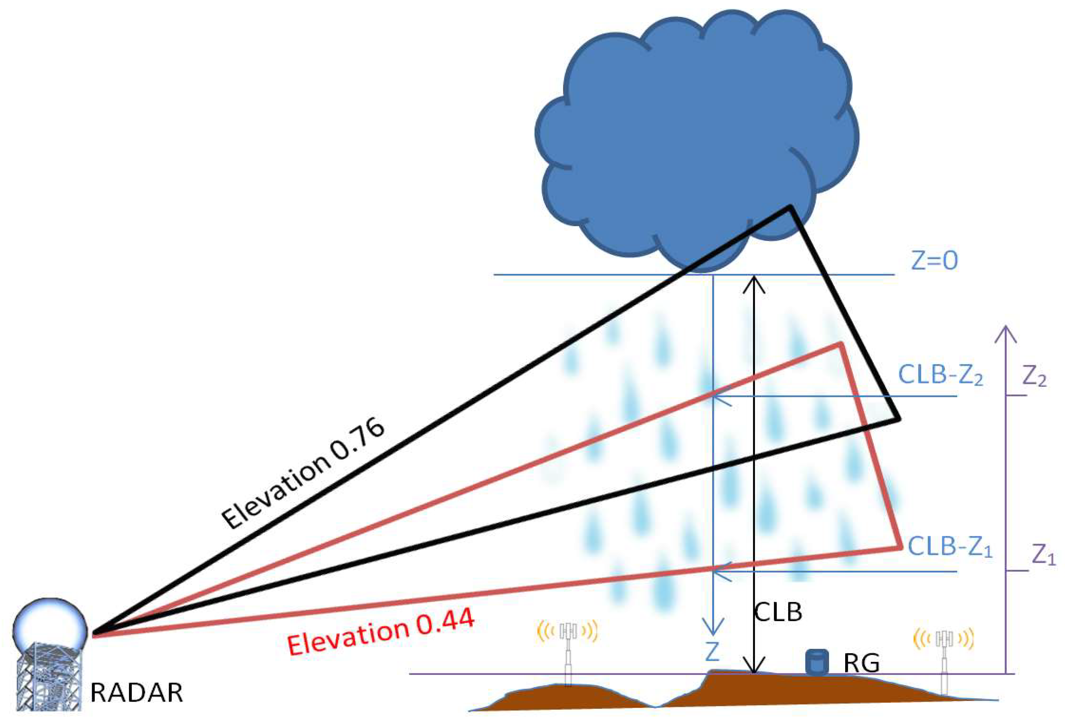
A diagram of the different measurement sources along the vertical axis Z, which actually goes from the CLB downwards, is depicted in Figure 1. To summarize the above, the samples vector can be represented, as: , where is the added measurement noise, but as one can see, it is problematic to differentiate between ; this is where additional prior knowledge is required. We suggest using the values of and that were derived according to the research done by Schlesinger et al. [17], and calculate by using the surrounding environment parameters . Next, we can present a new, and of lesser dimension, parameters vector:
and the samples vector is:
This problem’s solution is known and can easily be solved using a Least Squares Estimation (LSE) to extract . After doing so, our estimated values for and could be calculated by:
Finally, for the sake of validating the results, we can calculate, from the estimated parameters, the rain rate at the RG location and height, and compare it with the actual RG measurements. Given a RG height above ground level is less than a few meters and is roughly at ground level, the rain measurements in (mm/hr), when following Equation (5) and using the estimated parameters from Equation (9), can be represented as:
where is taken from the measurements at the specific weather station where the RG is located.
In the next section, the experiment and measurements selected in order to solve our estimation problem will be presented, as well as the corresponding results.
3. Results
3.1. The Experimental Setup
An experiment was performed in order to verify the validity of the suggested method for estimating and , thus effectively deriving the vertical profile of the rain-rates, as described in the previous section. The location of southern Israel was selected for our experiment site, as this region is of semi-arid nature, and thus can enable the occurrence of the Virga phenomenon. This location is at the vicinity of the city of Arad and of the site of Shani, and has a CML of 16 km length, deployed between Arad and Shani. The CML is situated at about 40 meters above the ground level, while recording maximum attenuations once every 15 min. As suggested in the previous section, we included measurements of the weather radar of the Israeli Meteorological Service (IMS); the IMS weather radar performs a complete scan, at different elevations, every five minutes. Two different radar elevation levels were relevant for the experiment: The first one observes at heights of between 355 and 1940 m, and the second one observes between 1275 and 2862 m above ground level for the selected experiment site. Once we were able to estimate the and using the CML attenuation measurements together with the weather radar, as suggested in the previous section, we were able to later derive the estimated values of rain rate at the RGs locations , with the corresponding humidity measurements for each RG location, and compare them with actual RG measurements. The experimental site holds two RGs for the sake of this validation, one near Arad, and the other near Shani, which samples the accumulated rain every 10 min. The experimental site, the mentioned CML, the weather radar, and the two RGs are shown in Figure 2.
The storms of 7–8 May 2014 and of 25–27 March 2016 were selected to be analyzed, since the months of March to May are generally dry in Israel in this region and the humidity could drop dramatically, thus creating good conditions for significant evaporation of rain drops, as discussed in the introduction.
In addition, since the CML records only the maximum attenuation every 15 min, and not instantaneous measurements, when deriving rain rates from CML samples, we had to use the power law parameters: , as was suggested recently [18]. In a recent study [18], a power law parameters calibration was performed to use maximum attenuation values of a CML, at the same test site location. The zero-level attenuation, when there is no actual rain, and is composed of the CML free path attenuation due to dry air, water vapor etc. [7], was measured prior to the onset of the selected storm events, and was deducted from the CML measurements during the storms.
Furthermore, when analyzing the weather radar measurements together with the CML derived rain rates, we had to address the different area spans and different timestamps of the samples. As a result, we used an averaging of 124 weather radar area cells above the CML location, which is called the Averaged Radar Cells Over Microwave Link (ARCOML) [19,20]. The weather radar cells that were selected for the ARCOML were of an area of about 125 m over 1 km, as the resolution of the radar is 125 m by 1°, and located above the CML path. In addition, when combining the samples of different timestamps and resolutions in time, we simply took the smallest common denominator, which is 30 min samples, when taking the resolution of the RGs into account.
To summarize, there are three different sources of measurement, the CML in addition to the weather radar beams at two elevations, while there two parameters we wish to estimate. Thus, as suggested in the previous section, we can now estimate and the by using LSE, while assuming the values of and as they were calculated previously [17] in addition to using the average of the relative humidity samples from the weather stations at Arad and Shani, which are located near the two ends of the CML used in this work. The estimation for and the was done every 30 min, and based on these estimation results, the near ground rain rates were estimated at the location of the two RGs every 30 min, using the relative humidity values for that RG location, via Equation (10).
3.2. Results
As described in the previous subsection, we conducted an experiment to calculate rain rates using multimodal measurements, in addition to using our suggested method, to interpolate measurements near the ground, at the Shani and Arad RGs locations. For each of the storms, we first estimated average rain rates at the and the itself for every 30-min interval. The estimation results for the storm of May 2014 is depicted in Figure 3 The estimated values for for the duration of the storm, above the CML, ranged between 0 and 18.2 mm/hr while the was varying up to 6 km and averaged at 3.18 km above ground level. The estimated values’ average is compared to actual observances at a somewhat nearby weather station (about 30 km away). However, while the estimated values for were physically within reason for this specific area and for a storm at this season, without access to real ground truth measurements for , we decided to validate the results by calculating the rain rate near ground at the RGs——and correlate it with actual RGs measurements. In Table 1, the correlation between the different measurement sources of rain rate (CML, RGs, ARCOML at two different elevations, and the suggested method estimated rain rate near ground—) is shown for the duration of 25 h on 7–8 May 2014 in southern Israel. The suggested method produced the highest correlation values, except for correlation with Arad RG, where the CML was slightly better correlated but by a very negligible margin: 0.9627 vs. 0.9615. When comparing the results of our method vs. Shani RG, we got a correlation of 0.5569, more than 10% over the second-best correlation value.
Figure 4 depicts the time series plot of all measurement sources for the May 2014 storm in addition to our suggested method. In comparison of our method with the CML, the ARCOML, or average of the two RGs, a higher correlation is found between our method and the CML than with the RGs. This could be attributed to the fact that the suggested method uses CML data, but also due to the pin-pointed location of the RGs, which is not representing its surrounding rain rate well, and the fact that both the CML and our method show results at near ground while the ARCOML does not. In Figure 4, it is also noticeable that when comparing the near ground methods to the ARCOML at the heights between 355 and 1940 m, as long as the relative humidity is around 50%, the radar beam overestimated rain rates as expected, and nearly matches the other methods in the second half of the storm when the relative humidity rises to near 100%. This is because the Virga effect diminishes significantly with 100% relative humidity.
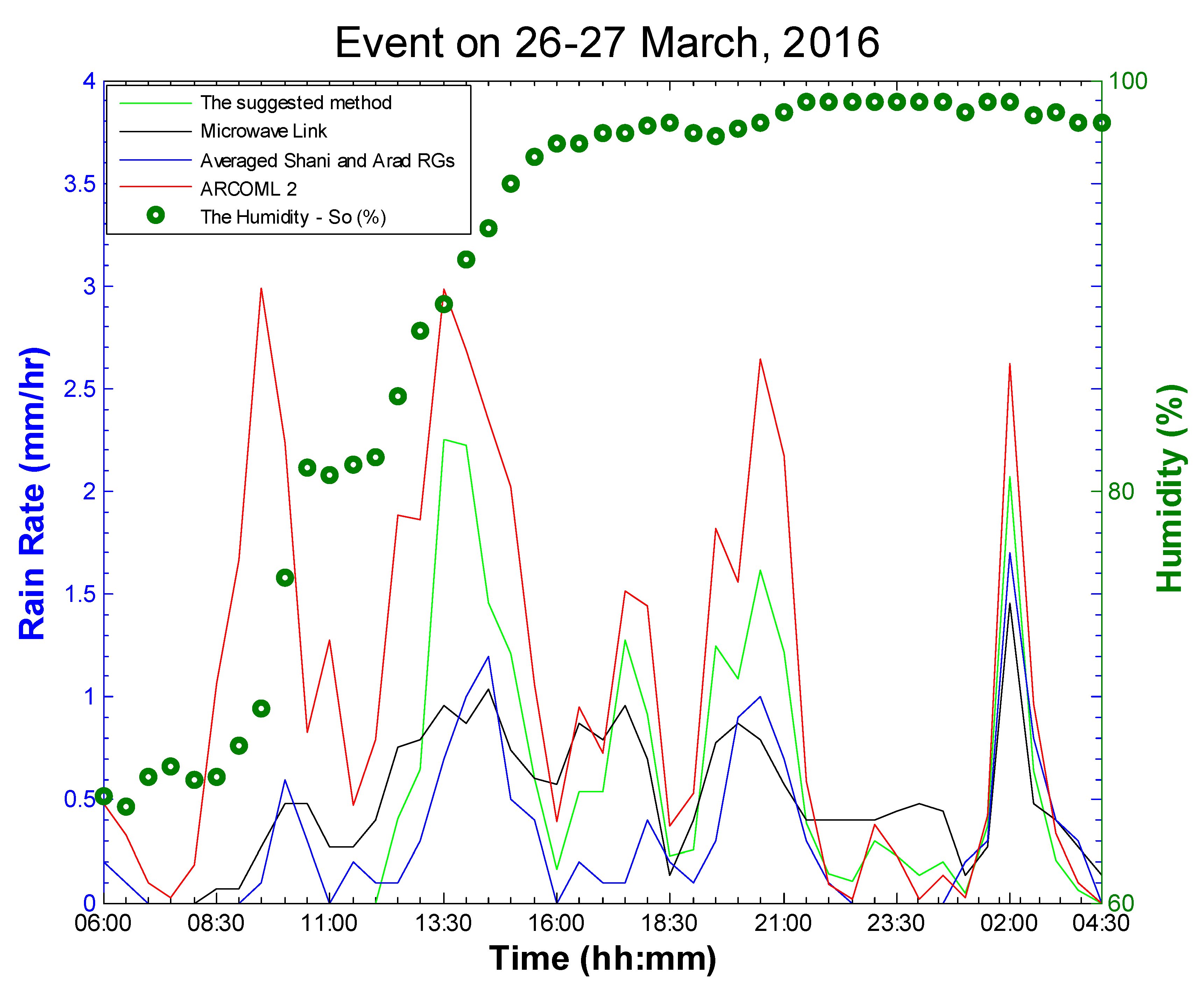
In addition to the storm event detailed above, we decided to include an additional event to test our suggested method. For the event of March 2016, the estimated values of are compared to actual (more accurate than for May 2014 storm) observances at a somewhat nearby weather station (about 30 km away) and are depicted in Figure 5; our estimated matches closely with those of the station. In Table 2, again, as we have no ground truth for , we calculated rain rates at ground level near the two rain gauges and calculated the correlations. Once again, our method provided the highest correlations, except when the rain gauges were compared to their own average (of course, this will show high correlation as for this storm, the correlation between the two rain gauges was high in the first place). In Figure 6, we show the temporal rain rate of the different sources for the March 2016 event, versus the humidity values, over 20 h on 26–27 March at southern Israel. Again, we see a good matching of our suggested method to the CML rain rates, and although it may seem that the values produced by our method are high, we need to remember that this storm produced very low rain rates, so the absolute difference between the ground sources (suggested method, rain gauges and ML) are low.
4. Conclusions
There are definitely some issues when trying to estimate near ground rain rates, using common currently used methods such as weather radar and RGs, in semi-arid regions. While RGs may produce relatively-accurate near-ground rain amounts, they are not necessarily representative of the surrounding rain amounts, particularly in a semi-arid region. And although the weather radar covers large areas with high resolution when measuring rain rates; some evaporation may occur when measuring at a high altitude above ground, and then the radar overestimates the rain rates at the ground level. In Figure 4, we observe both of these issues as we can clearly see that the RGs provide localized rain rates that do not match throughout the duration of the storm to the other methods, while the ARCOML shows significant over-estimations when the relative humidity is still low at around 50%. Moreover, when correlating Shani RG with Arad RG for the May 2014 storm, we get a value of 0.4768, emphasizing the pin-pointed representation of the RGs, when compared to the other methods.
In this research, we provided a method of overcoming these issues by using several radar beams at different heights, in conjunction with a near ground CML, which covers a long distance. The resulted method yielded the highest correlation values (or second best by a very small margin in one case) when compared to the RGs (in comparison to other methods).
Dealing with the lack of an accurate near-ground semi-arid precipitation monitoring method is one of the major goals of this work. The CMLs help us in researching and getting a better understanding of rain in semi-arid areas. In particular, the Virga phenomenon can be better understood, as well as the vertical profile of rain below the cloud base level. In this study, we have shown that the Virga phenomenon in semi-arid regions is neither uncommon nor negligible and thus cannot be disregarded when monitoring rain in these areas. We suggest a revolutionary tool that uses the already existing diversity of the CMLs in conjunction with the weather radar, which for the first time offers a solution to monitor near-ground precipitation, with the high resolution of the weather radar, for semi-arid regions by estimating the vertical profile of the rain rates and calculating the rain rates near the ground. This method of measuring near ground rain rates more accurately can assist in flash flood warnings [21], and in studying other weather phenomena in semi-arid regions. However, this study has its limitations: this research cannot provide test cases spanning over a few years, as the rain events for semi-arid regions are uncommon in Israel, and are limited to a few months a year.
Author Contributions
R.R. carried out the experiment. P.A. and H.M. contributed to the interpretation of the results. R.R. took the lead in writing the manuscript with input from all the authors. All authors provided critical feedback and helped shape the research, analysis and manuscript.
Funding
This research received no external funding.
Acknowledgments
We wish to thank the help of our friends within cellular network service providers: Cellcom, Pelephone, and PHI for providing us data over the last decade. In addition, we thank all members of our research team in Tel Aviv University, led by Hagit Messer and Pinhas Alpert for their cooperation and beneficial discussions.
Conflicts of Interest
The authors declare no conflict of interest.
References
- Olsen, R.O.; Rogers, D.V.; Hodge, D. The aRb relation in the calculation of rain attenuation. IEEE Trans. Antennas Propag. 1978, 26, 318–329. [Google Scholar] [CrossRef]
- Messer, H.; Zinevich, A.; Alpert, P. Environmental monitoring by wireless communication networks. Science 2006, 312, 713. [Google Scholar] [CrossRef] [PubMed]
- Messer, H. Rainfall Monitoring Using Cellular Networks [In the Spotlight]. IEEE Signal Process. Mag. 2007, 24, 144-142. [Google Scholar] [CrossRef]
- Leijnse, H.; Uijlenhoet, R.; Stricker, J.N.M. Rainfall measurement using radio links from cellular communication networks. Water Resour. Res. 2007, 43. [Google Scholar] [CrossRef] [Green Version]
- David, N.; Alpert, P.; Messer, H. Technical Note: Novel method for water vapour monitoring using wireless communication networks measurements. Atmos. Chem. Phys. 2009, 9, 2413–2418. [Google Scholar] [CrossRef] [Green Version]
- Harel, O.; Messer, H. Extension of the Mflrt to detect an unknown deterministic signal using multiple sensors, applied for precipitation detection. IEEE Signal Process. Lett. 2013, 20, 945–948. [Google Scholar] [CrossRef]
- Zinevich, A.; Alpert, P.; Messer, H. Estimation of rainfall fields using commercial microwave communication networks of variable density. Adv. Water Resour. 2008, 31, 1470–1480. [Google Scholar] [CrossRef]
- Goldshtein, O.; Messer, H.; Zinevich, A. Rain rate estimation using measurements from commercial telecommunications links. IEEE Trans. Signal Process. 2009, 57, 1616–1625. [Google Scholar] [CrossRef]
- Messer, H.; Sendik, O. A new approach to precipitation monitoring: A critical survey of existing technologies and challenges. IEEE Signal Process. Mag. 2015, 32, 110–122. [Google Scholar] [CrossRef]
- Liberman, Y.; Samuels, R.; Alpert, P.; Messer, H. New algorithm for integration between wireless microwave sensor network and radar for improved rainfall measurement and mapping. Atmos. Meas. Tech. 2014, 7, 3549–3563. [Google Scholar] [CrossRef] [Green Version]
- Evans, E.; Stewart, R.E.; Henson, W.; Saunders, K. On precipitation and Virga over three locations during the 1999–2004 Canadian Prairie drought. Atmos. Ocean 2011, 49, 366–379. [Google Scholar] [CrossRef]
- Fraser, A.B.; Bohren, C.F. Is Virga rain that evaporates before reaching the ground? Mon. Weather Rev. 1992, 120, 1565–1571. [Google Scholar] [CrossRef]
- Sassen, K.; Krueger, S.K. Toward an empirical definition of Virga: Comments on “Is virga rain that evaporates before reaching the ground?”. Mon. Weather Rev. 1993, 121, 2426–2428. [Google Scholar] [CrossRef]
- Ciach, G.J. Local random errors in tipping-bucket rain gauge measurements. J. Atmos. Ocean. Technol. 2003, 20, 752–759. [Google Scholar]
- Specific Attenuation Model for Rain for Use in Prediction Methods; ITU-R Recommendations; P Series Fasicle; ITU: Geneva, Switzerland, 2005.
- Millimeter Wave Propagation: Spectrum Management Implications. Available online: https://transition.fcc.gov/Bureaus/Engineering_Technology/Documents/bulletins/oet70/oet70a.pdf (accessed on 29 May 2018).
- Schlesinger, M.E.; Oh, J.H.; Rosenfeld, D. A parameterization of the evaporation of rainfall. Mon. Weather Rev. 1988, 116, 1887–1895. [Google Scholar] [CrossRef]
- Ostrometzky, J.; Raich, R.; Eshel, A.; Messer, H. Calibration of the attenuation-rain rate power-law parameters using measurements from commercial microwave networks. In Proceedings of the 2016 IEEE International Conference on Acoustics, Speech and Signal Processing (ICASSP), Shanghai, China, 20–25 March 2016; pp. 3736–3740. [Google Scholar]
- Eshel, A. Commercial Microwave Links and Radar Integration in Respect to Flash Floods in the Dead Sea Area. Master’s Thesis, Tel Aviv University, Tel Aviv, Israel, 2017. [Google Scholar]
- Raich, R. On the Use of Commercial Microwave Links for Rainfall Profile Estimation in Semi-Arid Areas. Master’s Thesis, Tel Aviv University, Tel Aviv, Israel, 2018. [Google Scholar]
- Rozalis, S.; Morin, E.; Yair, Y.; Price, C. Flash flood prediction using an uncalibrated hydrological model and radar rainfall data in a Mediterranean watershed under changing hydrological conditions. J. Hydrol. 2010, 394, 245–255. [Google Scholar] [CrossRef]
Figure 1.
A diagram of the different measurement sources in respect to the vertical axis Z. The picture depicts two radar beams at different elevation levels and gives an example of the heights the elevation of 0.44° observes: , , in respect to the Z-axis, which actually goes from the cloud base (ClB) downwards to the ground. On the ground level, we can see a rain gauge (RG) and cellular antennas of the CML.

Figure 2.
The experiment site area: Southern Israel, the weather radar of the Israeli Meteorological Service (IMS) (white target), Arad and Shani RGs (white triangles), and the commercial microwave link marked with two black antenna markers and the actual microwave link between them (purple).
Figure 2.
The experiment site area: Southern Israel, the weather radar of the Israeli Meteorological Service (IMS) (white target), Arad and Shani RGs (white triangles), and the commercial microwave link marked with two black antenna markers and the actual microwave link between them (purple).
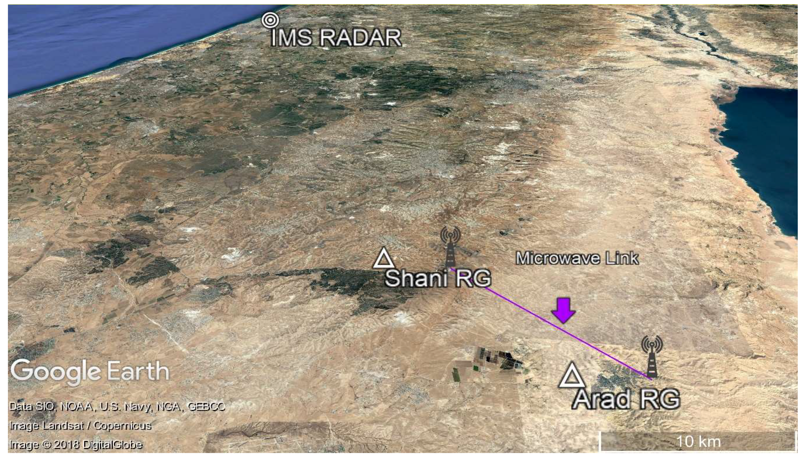
Figure 3.
May 2014 event, top subplot: estimated rain rates at the (brown) and the average humidity (green circles). Bottom subplot: estimated levels (brown stars), the average of the estimated (brown), the average of a real measurements nearby (blue), and the average humidity (green circles).
Figure 3.
May 2014 event, top subplot: estimated rain rates at the (brown) and the average humidity (green circles). Bottom subplot: estimated levels (brown stars), the average of the estimated (brown), the average of a real measurements nearby (blue), and the average humidity (green circles).
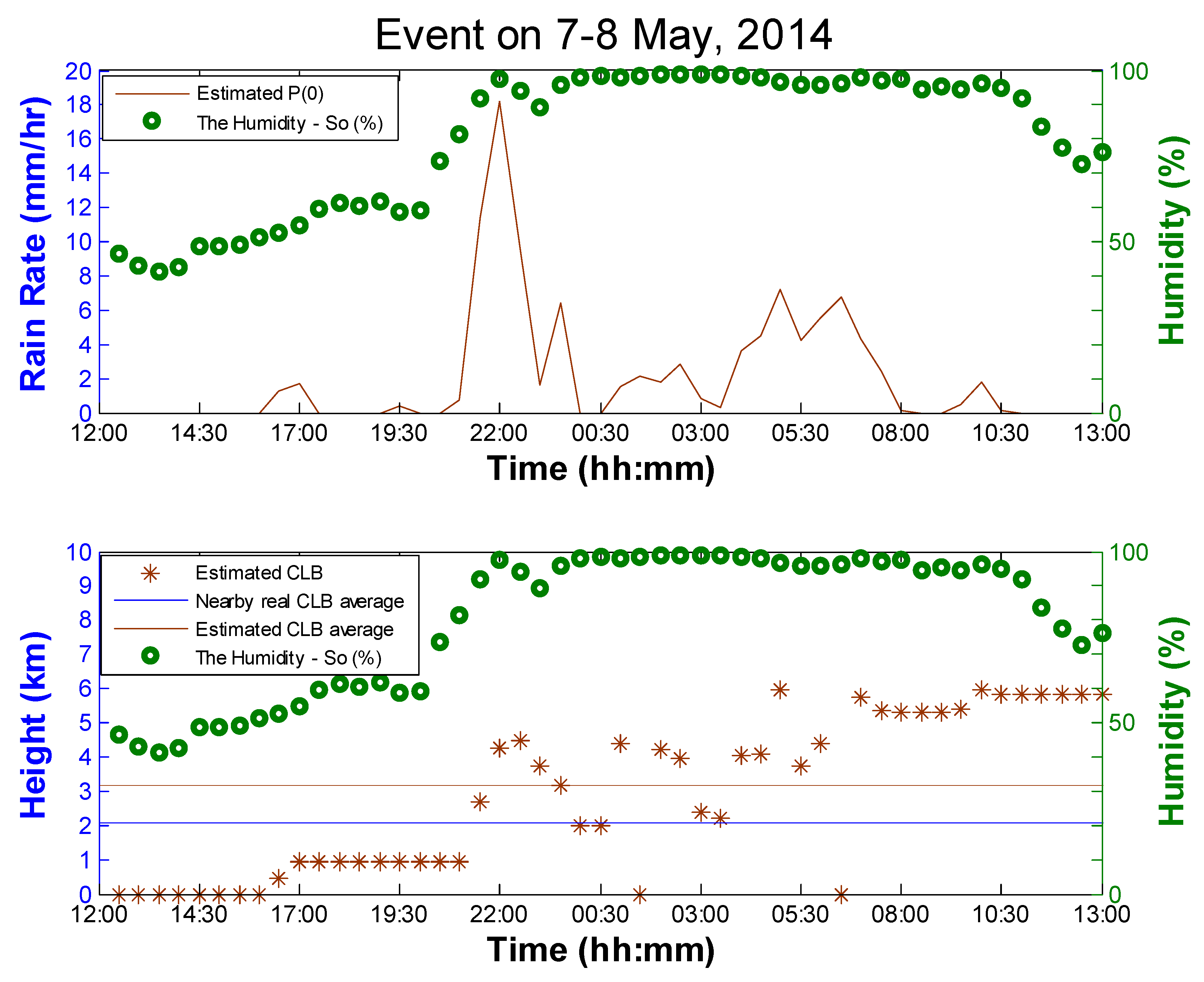
Figure 4.
The temporal rain rate according to the average of Arad and Shani RGs (in blue), the rain rate according to the microwave link (in black), the lower weather radar beam (ARCOML 1, in red), as well as according to the suggested method (in green) in correspondence with the event’s relative humidity averaged from measurements at the weather station in Arad and Shani, over 25 h on 7–8 May at southern Israel.
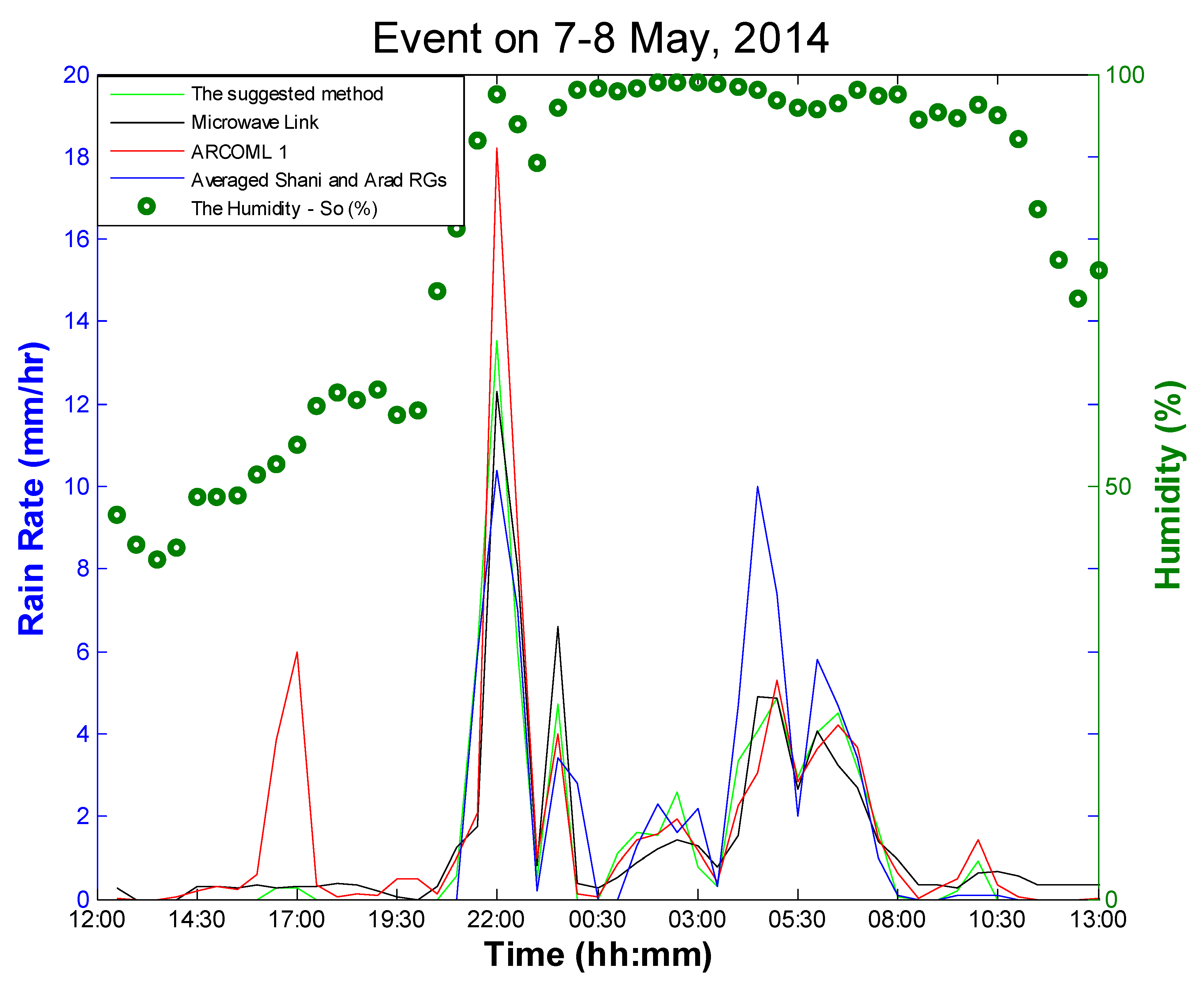
Figure 5.
March 2016 event, estimated levels (blue circles and dashes) and the ground truth of observed at nearby weather station (black).
Figure 5.
March 2016 event, estimated levels (blue circles and dashes) and the ground truth of observed at nearby weather station (black).
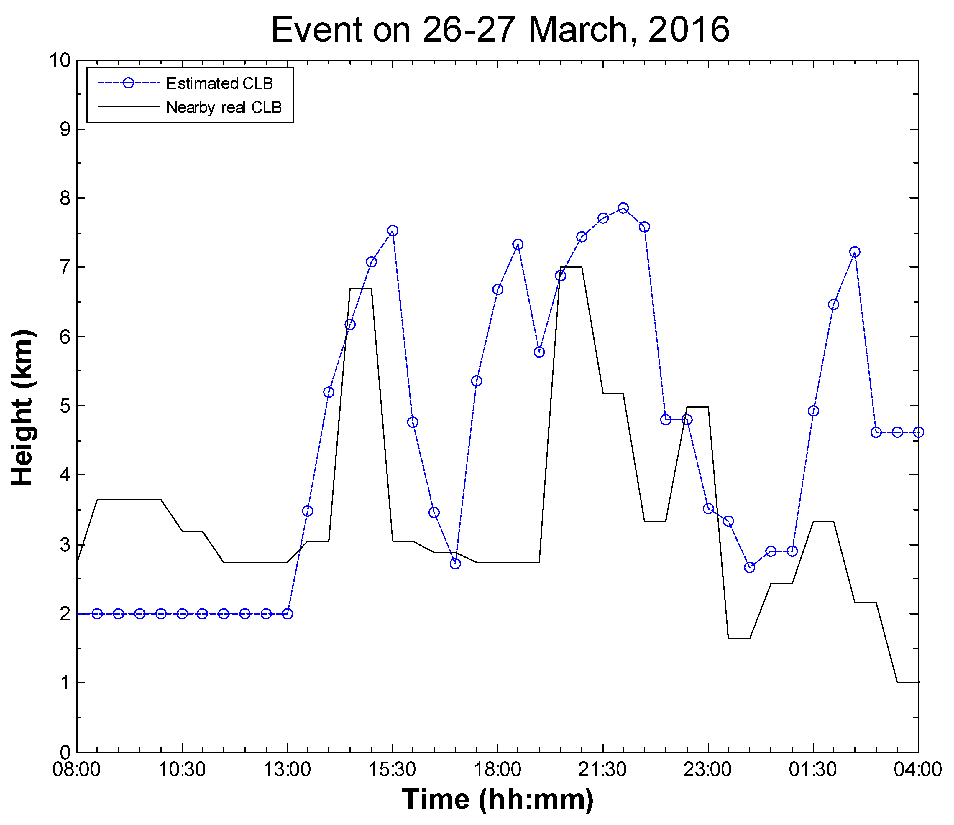
Figure 6.
The temporal rain rate according to the average of Arad and Shani RGs (in blue), the rain rate according to the microwave link (in black), the lower weather radar beam (ARCOML 2, in red), as well as according to the suggested method (in green) in correspondence with the event’s relative humidity averaged from the measurements at the weather station in Arad and Shani, over 20 h on 26–27 March at southern Israel.


Table 1.
The correlation of the ground truth rain rate measurements of Rain Gauges (RGs) in Arad, Shani and their average, with the different measurement sources for rain rate (RGs, Commercial Microwave Link (CML), Averaged Radar Cells Over Microwave Link (ARCOML) at two different elevations, and the suggested method of estimating rain rates near ground by combining radar and microwave link measurements) over the duration of 25 h on 7–8 May 2014 at the experiment site between the cities of Arad and Shani in southern Israel. Values marked in green show best values, values marked in yellow show second-best values for a specific column.
| Caption | Correlation with Shani RG | Correlation with Arad RG | Correlation with the Average of Arad & Shani RGs |
|---|---|---|---|
| Shani RG | 1 | 0.4768 | 0.8259 |
| Arad RG | 0.4768 | 1 | 0.8894 |
| CML | 0.4636 | 0.9627 | 0.8586 |
| ARCOML1 (0.35–1.94 km) | 0.3233 | 0.9060 | 0.7493 |
| ARCOML2 (1.28–2.86 km) | 0.4911 | 0.9385 | 0.8574 |
| The suggested method | 0.5569 | 0.9615 | 0.8926 |
Table 2.
The correlation of the ground truth rain rate measurements of rain gauges (RGs) in Arad, Shani and their average, with the different measurement sources for rain rate (RGs, commercial microwave link (CML), averaged radar cells over microwave link (ARCOML) at two different elevations, and the suggested method of estimating rain rates near ground by combining radar and microwave link measurements) over the duration of 20 h on 26–27 May 2016 at the experiment site between the cities of Arad and Shani in southern Israel. Values marked in green show best values, values marked at yellow show second best values, and third best marked in purple for a specific column.
| Caption | Correlation with Shani RG | Correlation with Arad RG | Correlation with the Average of Arad & Shani RGs |
|---|---|---|---|
| Shani RG | 1 | 0.6775 | 0.9300 |
| Arad RG | 0.6775 | 1 | 0.9003 |
| CML | 0.5956 | 0.6649 | 0.6909 |
| ARCOML1 (0.35–1.94 km) | 0.6650 | 0.6263 | 0.7028 |
| ARCOML2 (1.28–2.86 km) | 0.6443 | 0.5729 | 0.6608 |
| The suggested method | 0.6861 | 0.7543 | 0.7890 |
© 2018 by the authors. Licensee MDPI, Basel, Switzerland. This article is an open access article distributed under the terms and conditions of the Creative Commons Attribution (CC BY) license (http://creativecommons.org/licenses/by/4.0/).
Share and Cite
MDPI and ACS Style
Raich, R.; Alpert, P.; Messer, H. Vertical Precipitation Estimation Using Microwave Links in Conjunction with Weather Radar. Environments 2018, 5, 74. https://0-doi-org.brum.beds.ac.uk/10.3390/environments5070074
AMA Style
Raich R, Alpert P, Messer H. Vertical Precipitation Estimation Using Microwave Links in Conjunction with Weather Radar. Environments. 2018; 5(7):74. https://0-doi-org.brum.beds.ac.uk/10.3390/environments5070074
Chicago/Turabian StyleRaich, Roi, Pinhas Alpert, and Hagit Messer. 2018. "Vertical Precipitation Estimation Using Microwave Links in Conjunction with Weather Radar" Environments 5, no. 7: 74. https://0-doi-org.brum.beds.ac.uk/10.3390/environments5070074
Note that from the first issue of 2016, this journal uses article numbers instead of page numbers. See further details here.