Ecological Health Index: A Short Term Monitoring Method for Land Managers to Assess Grazing Lands Ecological Health


Abstract
:1. Introduction
2. Materials and Methods
2.1. Experimental Site
2.2. Ecological Health Index
- I = Index value (SSI, WCI, NCI, CDI or EFI),
- M = Max possible value of the total scores of related indicators,
- i = total scores of related indicators,
- D = Difference between max and min possible values of the total scores of related indicator.
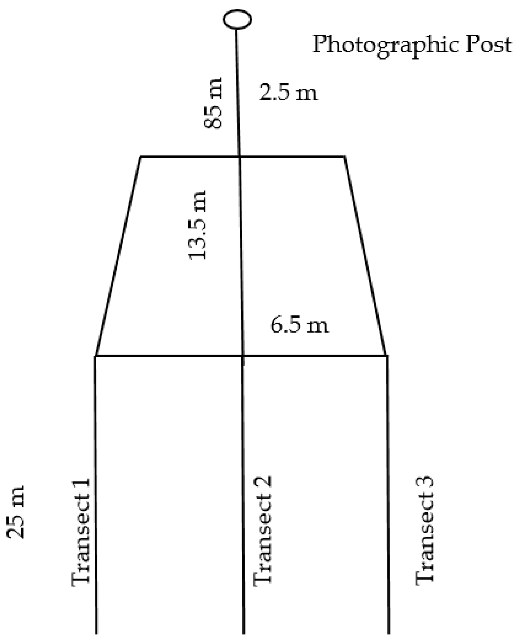
2.3. Long Term Fixed Transects
2.4. Statistical Analysis
3. Results
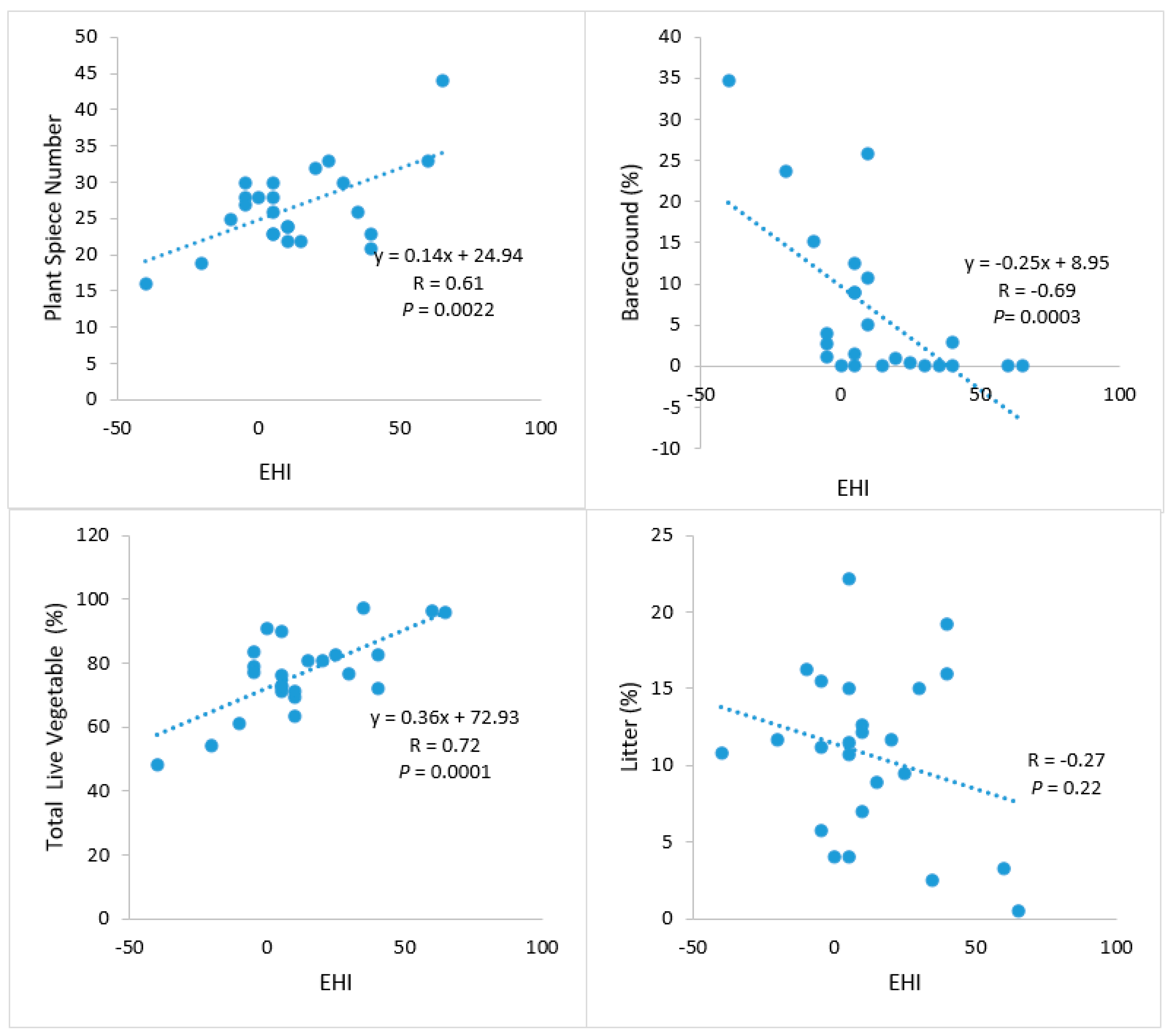
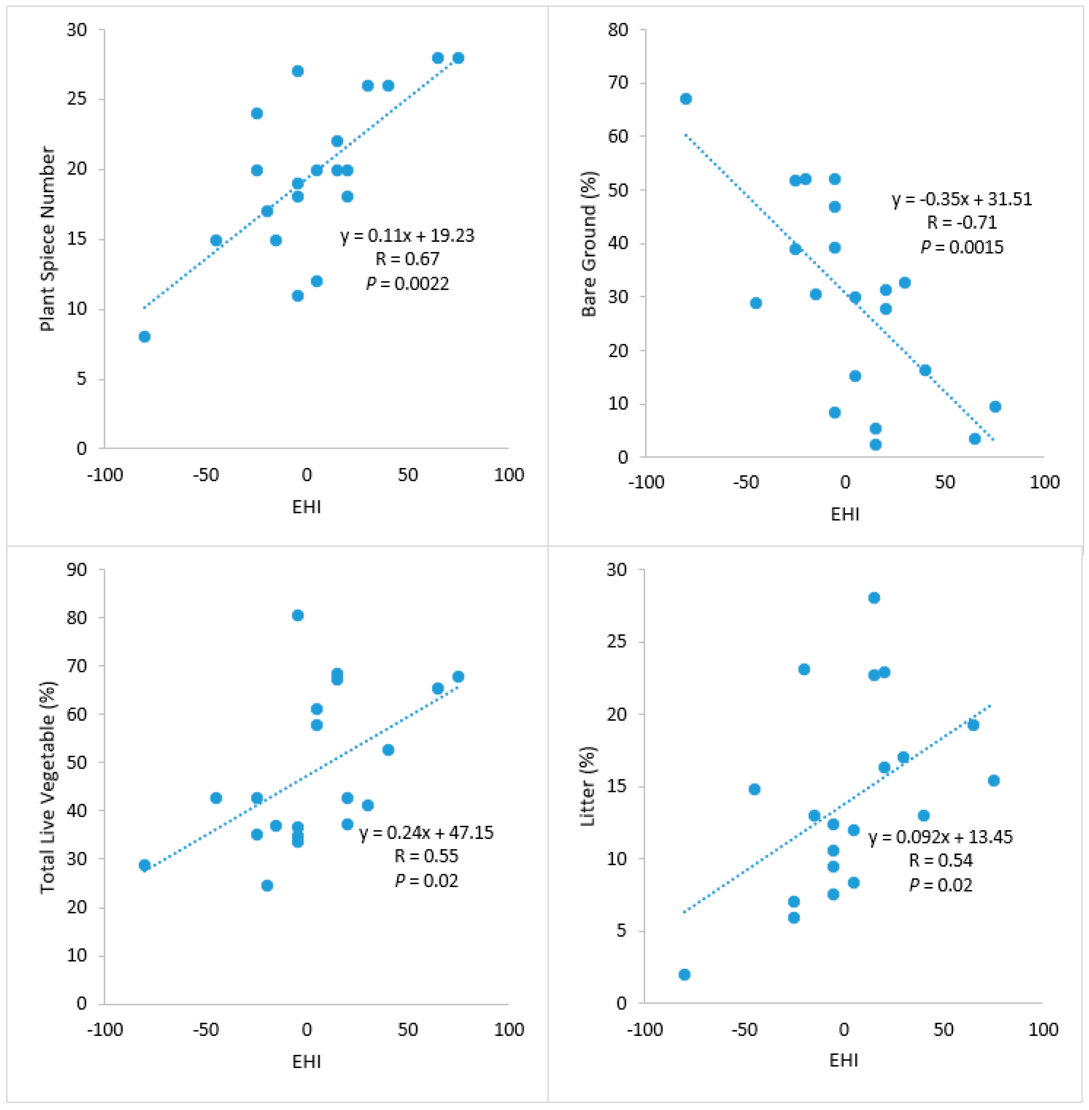
3.1. Ecological Health Index and Quantifiable Measurements
3.2. Carrying Capacity
4. Discussion
4.1. Ecological Health Index and Quantifiable Measurements
4.2. EHI and Carrying Capacity
5. Conclusions
Author Contributions
Funding
Acknowledgments
Conflicts of Interest
Appendix A

| Departure from Reference Sheet | ||||||||
|---|---|---|---|---|---|---|---|---|
| Num. | Atribute | Process Indicator | Score | N-S | S-M | M | M-E | E-T |
| 1 | Vegetation cover | % Vegetation cover | −10 to +10 | Total perennial vegetation cover exceeds 95% | Total perennial vegetation between 90–95% | Total perennial vegetation between 80–90% | Total perennial vegetation between 70–80% | Total perennial vegetation less than 70% |
| 10 | 5 | 0 | −5 | −10 | ||||
| 2 | Capping | Surface soil resistance | −10 to +10 | Loose soil or light capping that breaks easily with finger tip | Loose soil or light capping that breaks easily with finger tip | Loose soil or light capping that breaks easily with finger tip | Moderately hard capping requires pressure to break | Very hard capping requires metallic tool to break |
| 10 | 5 | 0 | −5 | −10 | ||||
| 3 | Wind erosion | Active blowout/deposition processes | 0 to −20 | Not present | Not present | Slight soil movement | Blowout/deposition areas cover 10–25% of the area | Blowout/deposition areas >25% of the area |
| Active pedestals | Not present | Not present | Few active active pedestals, hard to find | Active pedestals 5–10 cm deep | Pedestals abundant and active, more than 10 cm deep | |||
| Total | 0 | 0 | 0 | −10 | −20 | |||
| 4 | Water erosion | Active rills | 0 to −20 | Not present | Not present | Not present | Laminar erosion or active rills evident and well defined | Rill formation is severe and well defined throughout the site |
| Active water flows | Not present | Not present | Not present | Visible waterflows width < than 2 cm | Visible water flows, width > 2 cm | |||
| Active gullies | Not present | Not present | Not present | Active gullies present, low frequency | Active gullies frequent | |||
| Total | 0 | 0 | 0 | −10 | −20 | |||
| 5 | Litter incorporation | Litter/soil contact | 10 | More than 50% of the area with low incorporation | 20 to 50% of the area with low incorporation | Incorporation null | Incorporation null | Incorporation null |
| 10 | 5 | 0 | 0 | 0 | ||||
| 6 | Living organisms | Evidence of microfauna | 10 | Abundant presence of dung beetles, aunts, spiders and other species | Moderate presence of dung beetles, aunts, spiders and other species | Scarce presence of dung beetles, aunts, spiders and other species | Scarce presence of dung beetles, aunts, spiders and other species | Scarce presence of dung beetles, aunts, spiders and other species |
| 10 | 5 | 0 | 0 | 0 | ||||
| 7 | Dung decomposition | Dung age structure | 10 | Only fresh dung is present. Fast cycling | Fresh and old dung mixed | Most of dung patches are more than 1 year old (mummified) | Most of dung patches are more than 1 year old (mummified) | Most of dung patches are more than 1 year old (mummified) |
| 10 | 5 | 0 | 0 | 0 | ||||
| 8 | Tussock | Tussock in good condition | −10 to 10 | >30% | 20–30% | 10–20% | <10% | 0 |
| Decadent tussock | <20% | 20–30% | 30–40% | 40–50% | >50% | |||
| Total | 10 | 5 | 0 | −5 | −10 | |||
| 9 | Decreasers | Frequency | 10 | >10 plants/m2 | 1–10 plants/m2 | <1 plant/m2 | Decreaser species absent | Decreaser species absent |
| 10 | 5 | 0 | 0 | 0 | ||||
| 10 | Key species | Plants in good condition | −20 to 20 | >50% | 30–50% | 10–30% | <10% | <10% |
| Decadent plants | <10% | 10–30% | 30–50% | 50–70% | >70% | |||
| 20 | 10 | 0 | −10 | −20 | ||||
| 11 | Shrubs | Plants in good condition | −10 to 10 | >50% | 30–50% | 10–30% | <10% | Not observed |
| Decadent plants | <10% | 10–20% | 20–30% | 30–50% | >50% | |||
| 10 | 5 | 0 | −5 | −10 | ||||
| 12 | Invaders | Abundance | Not observed | Not observed | Not observed | Moderate presence of young plants of Empetrum rubrum, Azzorella or Hieracium pilosella | Abundant presence of young plants of Empetrum rubrum, Azzorella or Hieracium pilosella | |
| 0 | 0 | 0 | −10 | −20 | ||||
| 13 | Total production | % of Reference area | −10 to 10 | More than 75% of reference area | 60–75% of reference area | 50–60% of reference area | 25–50% of reference area | <25% of reference area |
| 10 | 5 | 0 | −5 | −10 | ||||
| 110 | 55 | 0 | −65 | −130 | ||||
| N-S | Nil to slight | |||||||
| S-M | Slight to moderate | |||||||
| M | Moderate | |||||||
| M-E | Moderate to extreme | |||||||
| E-T | Extreme to total | |||||||
| FUNCTIONAL GROUPS | ||||||||
| TUSSOCK | Tall, rough bunchgrasses—Provide structure, produce litter and have deep roots | |||||||
| Decreasers | Plants that disappear under continuous grazing. Usually broad leaved, more mesic grasses and native legumes | |||||||
| Key Species | Abundant, preferred species. Determine most of the high quality forage | |||||||
| Shrubs | Woody plants that create niches and provide forage in winter time | |||||||
| Invaders | (old term for contextually undesirable species). Plants that are emblematic of an undesired transition. Mostly exotic or unpalatable native woody plants | |||||||
| Departure from Reference Sheet | ||||||||
|---|---|---|---|---|---|---|---|---|
| Num. | Atribute | Process Indicator | Score | N-S | S-M | M | M-E | E-T |
| 1 | Litter | %Cover | 0 to 10 | Grade 3 litter or more, more than 15% cover | Grade 3 Litter: 10–15% cover | Grade 2 Litter: 1–10% cover | Grade 1 Litter: <1% cover | Grade 1 Litter: <1% cover |
| 10 | 5 | 0 | 0 | 0 | ||||
| 2 | Vegetation cover | % Vegetation cover | −10 to +10 | Perennial Vegetation cover exceeds 60% Bare ground less than 20% | Perennial Vegetation cover 55–60%. Bare Ground 20–25% | Perennial Vegetation cover 55–60%. Bare Ground 25–35% | Perennial Vegetation cover 40–55%. Bare Ground 35–50% | Perennial Vegetation cover <40%. Bare Ground >50% |
| 10 | 5 | 0 | −5 | −10 | ||||
| 3 | Capping | Surface soil resistance | −10 to +10 | Loose soil or light capping that breaks easily with finger tip | Loose soil or light capping that breaks easily with finger tip | Loose soil or light capping that breaks easily with finger tip | Moderately hard capping requires pressure to break | Very hard capping requires metallic tool to break |
| 0 | 0 | 0 | −5 | −10 | ||||
| 4 | Wind erosion | Active blowout/deposition processes | 20 to −20 | Not present (Grade 4) | Grade 4 predominant, less than 30% Grade 3 | Grade 3 predominant | Blowout/deposition areas cover 10–25% of the area | Blowout/deposition areas >25% of the area (Grade 2) |
| Active pedestals | Not present (Grade 4) | Not present (Grade 4) | Few active active pedestals, hard to find (Grade 3) | Active pedestals 5–10 cm deep (Grade 2) | Pedestals abundant and active, more than 10 cm deep | |||
| Total | 20 | 10 | 0 | −10 | −20 | |||
| 5 | Water erosion | Active rills | 0 to −20 | Not present (Grade 4) | Not present (Grade 4) | Not present (Grade 4) | Laminar erosion or active rills evident and well defined | Rill formation is severe and well defined throughout the site |
| Active water flows | Not present (Grade 4) | Not present (Grade 4) | Not present (Grade 4) | Visible waterflows width < than 2 cm (Grade 3) | Visible water flows, width > 2 cm (Grade 2 and 1) | |||
| Active gullies | Not present (Grade 4) | Not present (Grade 4) | Not present (Grade 4) | Active gullies present, low frequency | Active gullies frequent | |||
| Total | 0 | 0 | 0 | −10 | −20 | |||
| 6 | Biological crust | Cover | 0 to 10 | >5% (Grade 3) | Between 1–5% (Grade 2) | <1% (Grade1) | Not Present (Grade 0) | Not Present (Grade 0) |
| 10 | 5 | 0 | 0 | 0 | ||||
| 7 | Litter incorporation | Litter/soil contact | 0 to 10 | More than 50% of the area with low incorporation | 20 to 50% of the area with low incorporation | Incorporation null | Incorporation null | Incorporation null |
| 10 | 5 | 0 | 0 | 0 | ||||
| 8 | Living organisms | Evidence of microfauna | −10 to 10 | Moderate presence of dung beetles, aunts, spiders and other species | Scarce presence of dung beetles, aunts, spiders and other species | Scarce presence of dung beetles, aunts, spiders and other species | Scarce presence of dung beetles, aunts, spiders and other species | Scarce presence of dung beetles, aunts, spiders and other species |
| 5 | 0 | 0 | 0 | 0 | ||||
| 9 | Dung decomposition | Dung age structure | 0 to 10 | Does not apply | Does not apply | Does not apply | Does not apply | Does not apply |
| 0 | 0 | 0 | 0 | 0 | ||||
| 10 | Tussock | Tussock in good condition | −10 to 10 | >40% | 25–40% | 10–25% | <10% | Not observed |
| Decadent tussock | <10% | 10–25% | 25–40% | 40–60% | >60% | |||
| Total | 10 | 5 | 0 | −5 | −10 | |||
| 11 | Decreasers | Frequency | 0 to 10 | Very abundant >10 plants/m2 | 1–10 plants per m2 | less than 1 plant/m2 | Decreasers are absent | Decreasers are absent |
| 10 | 5 | 0 | 0 | 0 | ||||
| 12 | Key species | Plants in good condition | −20 to 20 | >40% | 25–40% | 10–25% | <10% | Not observed |
| Decadent plants | <10% | 10–25% | 25–40% | 40–60% | >60% | |||
| 20 | 10 | 0 | −10 | −20 | ||||
| 13 | Shrubs | Plants in good condition | −10 to 10 | >50% | 30–50% | 10–30% | <10% | Not observed |
| Decadent plants | <10% | 10–20% | 20–30% | 30–50% | >50% | |||
| 10 | 5 | 0 | −5 | −10 | ||||
| 14 | Invaders | Abundance | 0 to −20 | Not observed | Not observed | Not observed | Rare to moderate presence of young plants of Stipa sp, Nassauvia and Acaena | Frequent presence of young plants of Stipa sp, Nassauvia and Acaena |
| 0 | 0 | 0 | −10 | −20 | ||||
| 15 | Total production | % of Reference area | More than 75% of Reference Area | 60–75% of Reference Area | 50–60% of Reference Area | 25–50% of Reference Area | <25% of Reference Area | |
| 10 | 5 | 0 | −5 | −10 | ||||
| 125 | 60 | 0 | −65 | −130 | ||||
References
- Follett, R.F.; Reed, D.A. Soil carbon sequestration in grazing lands: Societal benefits and policy implications. Rangel. Ecol. Manag. 2010, 63, 4–15. [Google Scholar] [CrossRef]
- Thornton, P.K. Livestock production: Recent trends, future prospects. Philos. Trans. R. Soc. Lond. B Biol. Sci. 2010, 365, 2853–2867. [Google Scholar] [CrossRef] [PubMed]
- Oba, G.; Vetaas, O.R.; Stenseth, N.C. Relationships between biomass and plant species richness in arid-zone grazinglands. J. Appl. Ecol. 2001, 38, 836–845. [Google Scholar] [CrossRef]
- Parkpian, P.; Leong, S.T.; Laortanakul, P.; Thunthaisong, N. Regional monitoring of lead and cadmium contamination in a tropical grazingland site, Thailand. Environ. Monit. Assess. 2003, 85, 157–173. [Google Scholar] [CrossRef] [PubMed]
- Veblen, K.E.; Pyke, D.A.; Aldridge, C.L.; Casazza, M.L.; Assal, T.J.; Farinha, M.A. Monitoring of livestock grazing effects on Bureau of Land Management land. Rangel. Ecol. Manag. 2014, 67, 68–77. [Google Scholar] [CrossRef]
- Slimani, H.; Aidoud, A.; Roze, F. 30 Years of protection and monitoring of a steppic rangeland undergoing desertification. J. Arid Environ. 2010, 74, 685–691. [Google Scholar] [CrossRef]
- USDA NRCS. Inventorying and Monitoring Grazing Land Resources. In National Range and Pasture Handbook; USDA: Washington, DC, USA, 2006. Available online: https://directives.sc.egov.usda.gov/OpenNonWebContent.aspx?content=17739.wba (accessed on 27 June 2018).
- Pickup, G.; Bastin, G.N.; Chewings, V.H. Remote-sensing-based condition assessment for nonequilibrium rangelands under large-scale commercial grazing. Ecol. Appl. 1994, 4, 497–517. [Google Scholar] [CrossRef]
- Hill, J.; Hostert, P.; Tsiourlis, G.; Kasapidis, P.; Udelhoven, T.; Diemer, C. Monitoring 20 years of increased grazing impact on the Greek island of Crete with earth observation satellites. J. Arid Environ. 1998, 39, 165–178. [Google Scholar] [CrossRef]
- Del Barrio, G.; Puigdefabregas, J.; Sanjuan, M.E.; Stellmes, M.; Ruiz, A. Assessment and monitoring of land condition in the Iberian Peninsula, 1989–2000. Remote Sens. Environ. 2010, 114, 1817–1832. [Google Scholar] [CrossRef]
- Martin, R.; Müller, B.; Linstädter, A.; Frank, K. How much climate change can pastoral livelihoods tolerate? Modelling rangeland use and evaluating risk. Glob. Environ. Chang. 2014, 24, 183–192. [Google Scholar] [CrossRef]
- Gessesse, B.; Bewket, W.; Bräuning, A. Model-based characterization and monitoring of runoff and soil erosion in response to land use/land cover changes in the Modjo watershed, Ethiopia. Land Degrad. Dev. 2015, 26, 711–724. [Google Scholar] [CrossRef]
- Henderson, B.B.; Gerber, P.J.; Hilinski, T.E.; Falcucci, A.; Ojima, D.S.; Salvatore, M.; Conant, R.T. Greenhouse gas mitigation potential of the world’s grazinglands: Modeling soil carbon and nitrogen fluxes of mitigation practices. Agric. Ecosyst. Environ. 2015, 207, 91–100. [Google Scholar] [CrossRef]
- Kosmas, C.; Kairis, O.; Karavitis, C.; Ritsema, C.; Salvati, L.; Acikalin, S.; Alcalá, M.; Alfama, P.; Atlhopheng, J.; Barrera, J.; et al. Evaluation and selection of indicators for land degradation and desertification monitoring: Methodological approach. Environ. Manag. 2014, 54, 951–970. [Google Scholar] [CrossRef] [PubMed]
- Čuček, L.; Klemeš, J.J.; Kravanja, Z. A review of footprint analysis tools for monitoring impacts on sustainability. J. Clean. Prod. 2012, 34, 9–20. [Google Scholar] [CrossRef]
- Pyke, D.A.; Herrick, J.E.; Shaver, P.; Pellant, M. Rangeland health attributes and indicators for qualitative assessment. J. Range Manag. 2002, 55, 584–597. [Google Scholar] [CrossRef]
- Pellant, M.; Shaver, P.; Pyke, D.; Herrick, J. Interpreting Indicators of Rangeland Health, Version 4; Technical Reference 1734-6; US Department of Interior, Bureau of Land Management, National Science and Technology Center: Denver, CO, USA, 2005; 122p.
- Herrick, J.E.; Bestelmeyer, B.T.; Archer, S.; Tugel, A.J.; Brown, J.R. An integrated framework for science-based arid land management. J. Arid Environ. 2006, 65, 319–335. [Google Scholar] [CrossRef]
- Schwilch, G.; Bestelmeyer, B.; Bunning, S.; Critchley, W.; Herrick, J.; Kellner, K.; Liniger, H.P.; Nachtergaele, F.; Ritsema, C.J.; Schuster, B.; et al. Experiences in monitoring and assessment of sustainable land management. Land Degrad. Dev. 2011, 22, 214–225. [Google Scholar] [CrossRef]
- Toevs, G.R.; Karl, J.W.; Taylor, J.J.; Spurrier, C.S.; Karl, M.S.; Bobo, M.R.; Herrick, J.E. Consistent indicators and methods and a scalable sample design to meet assessment, inventory, and monitoring information needs across scales. Rangelands 2011, 33, 14–20. [Google Scholar] [CrossRef]
- Mitchell, J.E. Criteria and Indicators for Sustainable Rangeland Management; Cooperative Extension Service Publication SM-56; University of Wyoming: Laramie, WY, USA, 2010; p. 227. [Google Scholar]
- Ludwig, J.A.; Bastin, G.N.; Eager, R.W.; Karfs, R.; Ketner, P.; Pearce, G. Monitoring Australian rangeland sites using landscape function indicators and ground-and remote-based techniques. Environ. Monit. Assess. 2000, 64, 167–178. [Google Scholar] [CrossRef]
- Borrelli, P.; Oliva, G. Evaluación de Pastizales. Capítulo 6. In Ganadería Ovina Sustentable en la Patagonia Austral; Borrelli, P., Oliva, G., Eds.; Centro Regional Patagonia Sur INTA: Río Gallegos: Santa Cruz, Argentina, 2001. [Google Scholar]
- Tongway, D.J.; Hindley, N.L. Landscape Function Analysis: Procedures for Monitoring and Assessing Landscapes with Special Reference to Minesite and Rangelands; CSIRO: Canberra, Australia, 2004; 80p. [Google Scholar]
- Bartley, R.; Roth, C.H.; Ludwig, J.; McJannet, D.; Liedloff, A.; Corfield, J.; Hawdon, A.; Abbott, B. Runoff and erosion from Australia’s tropical semi-arid rangelands: Influence of ground cover for differing space and time scales. Hydrol. Process. 2006, 20, 3317–3333. [Google Scholar] [CrossRef]
- Read, Z.J.; King, H.P.; Tongway, D.J.; Ogilvy, S.; Greene, R.S.B.; Hand, G. Landscape function analysis to assess soil processes on farms following ecological restoration and changes in grazing management. Eur. J. Soil Sci. 2016, 67, 409–420. [Google Scholar] [CrossRef]
- Van der Walt, L.; Cilliers, S.S.; Kellner, K.; Tongway, D.; Van Rensburg, L. Landscape functionality of plant communities in the Impala Platinum mining area, Rustenburg. J. Environ. Manag. 2012, 113, 103–116. [Google Scholar] [CrossRef] [PubMed]
- Canfield, R.H. Application of the line interception method in sampling range vegetation. J. For. 1941, 39, 388–394. [Google Scholar]
- Tothill, J.C.; Hargreaves, J.N.G.; Jones, R.M.; McDonald, C.K. BOTANAL—A comprehensive sampling and computing procedure for estimating pasture yield and composition. 1. Field sampling. Trop. Agron. Tech. Memo. 1992, 78, 1–24. Available online: https://www.researchgate.net/profile/Cam_Mcdonald/publication/303169091_BOTANAL_A_comprehensive_sampling_procedure_for_estimating_pasture_yield_and_composition_I_Field_sampling/links/5a3a12f4458515889d2bd450/BOTANAL-A-comprehensive-sampling-procedure-for-estimating-pasture-yield-and-composition-I-Field-sampling.pdf (accessed on 30 May 2018).
- Buckland, S.T.; Anderson, D.R.; Burnham, K.P.; Laake, J.L.; Borchers, D.L.; Thomas, L. Introduction to Distance Sampling Estimating Abundance of Biological Populations; Oxford University Press: New York, NY, USA, 2001. [Google Scholar]
- Borrelli, P.F.; Boggio, P.; Sturzenbaum, M.; Paramidani, R.; Heinken, C.; Pague, M. Stevens and A. Nogués. Grassland Regeneration and Sustainable Standard (GRASS); The Nature Conservancy: Arlington County, VA, USA, 2012; p. 109. Available online: http://www.fao.org/fileadmin/user_upload/nr/sustainability_pathways/docs/GRASS%20english.pdf (accessed on 20 June 2018).
- Oliva, G.; Gaitán, J.; Bran, D.; Nakamatsu, V.; Salomone, J.; Buono, G.; Escobar, J.; Frank, F.; Ferrante, D.; Humano, G.; et al. Monitoreo Ambiental Para Regiones Áridas y Semiáridas. Available online: http://gefpatagonia.ambiente.gob.ar/archivos/web/MSEAySACDP/file/MARAS_Manual_mayo_2010.pdf (accessed on 15 May 2018).
- Halloy, S.; Ibañez, M.; Yager, K. Point and flexible area sampling for rapid inventories of biodiversity status. Ecología en Bolivia 2011, 46, 46–56. [Google Scholar]
- Asbjornsen, H.; Hernandez-Santana, V.; Liebman, M.; Bayala, J.; Chen, J.; Helmers, M.; Ong, C.K.; Schulte, L.A. Targeting perennial vegetation in agricultural landscapes for enhancing ecosystem services. Renew. Agric. Food Syst. 2014, 29, 101–125. [Google Scholar] [CrossRef]
- Symstad, A.J.; Jonas, J.L. Incorporating biodiversity into rangeland health: Plant species richness and diversity in Great Plains grasslands. Rangel. Ecol. Manag. 2011, 64, 555–572. [Google Scholar] [CrossRef]
- Zavaleta, E.S.; Pasari, J.R.; Hulvey, K.B.; Tilman, G.D. Sustaining multiple ecosystem functions in grassland communities requires higher biodiversity. Proc. Natl. Acad. Sci. USA 2010, 107, 1443–1446. [Google Scholar] [CrossRef] [Green Version]
- Allan, E.; Manning, P.; Alt, F.; Binkenstein, J.; Blaser, S.; Blüthgen, N.; Böhm, S.; Grassein, F.; Hölzel, N.; Klaus, V.H.; et al. Land use intensification alters ecosystem multifunctionality via loss of biodiversity and changes to functional composition. Ecol. Lett. 2015, 18, 834–843. [Google Scholar] [CrossRef]
- Hallett, L.M.; Stein, C.; Suding, K.N. Functional diversity increases ecological stability in a grazed grassland. Oecologia 2017, 183, 831–840. [Google Scholar] [CrossRef]
- Papanastasis, V.P.; Bautista, S.; Chouvardas, D.; Mantzanas, K.; Papadimitriou, M.; Mayor, A.G.; Koukioumi, P.; Papaioannou, A.; Vallejo, R.V. Comparative assessment of goods and services provided by grazing regulation and reforestation in degraded Mediterranean rangelands. Land Degrad. Dev. 2015, 28, 1178–1187. [Google Scholar] [CrossRef]
- Toledo, D.; Sanderson, M.; Herrick, J.; Goslee, S. An integrated approach to grazingland ecological assessments and management interpretations. J. Soil Water Conserv. 2014, 69, 110A–114A. [Google Scholar] [CrossRef] [Green Version]
- Weber, K.T.; Gokhale, B.S. Effect of grazing on soil-water content in semiarid rangelands of southeast Idaho. J. Arid Environ. 2011, 75, 464–470. [Google Scholar] [CrossRef]
- Shamoot, S.; McDonald, L.; Bartholomew, W.V. Rhizo-deposition of organic debris in soil. Soil Sci. Soc. Am. J. 1968, 32, 817–820. [Google Scholar] [CrossRef]
- Descroix, L.; Viramontes, D.; Vauclin, M.; Barrios, J.G.; Esteves, M. Influence of soil surface features and vegetation on runoff and erosion in the Western Sierra Madre (Durango, Northwest Mexico). Catena 2001, 43, 115–135. [Google Scholar] [CrossRef]
- Kachergis, E.; Rocca, M.E.; Fernandez-Gimenez, M.E. Indicators of ecosystem function identify alternate states in the sagebrush steppe. Ecol. Appl. 2011, 21, 2781–2792. [Google Scholar] [CrossRef]
- Waldron, B.L.; Greenhalgh, L.K.; ZoBell, D.R.; Olson, K.C.; Davenport, B.W.; Palmer, M.D. Forage Kochia Increases Nutritional Value, Carrying Capacity, and Livestock Performance on Semiarid Rangelands. Forage Grazinglands 2011, 9. [Google Scholar] [CrossRef]
- Sanderson, M.A.; Skinner, R.H.; Barker, D.J.; Edwards, G.R.; Tracy, B.F.; Wedin, D.A. Plant species diversity and management of temperate forage and grazing land ecosystems. Crop Sci. 2004, 44, 1132–1144. [Google Scholar] [CrossRef]


| Farm Name | Hectarage (Ha) | Monitored Subsidiaries within Farm | Year of Monitoring | Average Rainfall (mm) | Temperature (°C) |
|---|---|---|---|---|---|
| HMS | |||||
| Monte Dinero | 8000 | 1 | 2011 | 270 | 6.5 |
| Morro Chico | 26,025 | 2 | 2012 | 300 | 5.5 |
| Namuncura | 22,135 | 4 | 2012 | 250 | 5 |
| Rupai Pacha | 25,000 | 2 | 2012 | 200 | 5 |
| Viamonte | 40,600 | 1 | 2012 | 400 | 5 |
| Punta Delgada | 93,000 | 6 | 2013 | 250 | 6.5 |
| Teraike | 29,605 | 3 | 2013 | 400 | 6 |
| Pamela Christian | 9018 | 3 | 2013 | 400 | 6 |
| Armonia | 8000 | 2 | 2014 | 350 | 6 |
| SG | |||||
| La Paulina | 4306 | 2 | 2012 | 250 | 8 |
| Numancia | 23,000 | 5 | 2012 | 400–600 | 8 |
| Bajada de los Orientales | 56,000 | 3 | 2012 | 200 | 7 |
| El Amanecer | 4661 | 1 | 2012 | 350 | 8 |
| El Cronometro | 4746 | 2 | 2012 | 350 | 8 |
| La Legua | 2500 | 1 | 2012 | 250 | 8 |
| Montoso | 2500 | 1 | 2012 | 250 | 9 |
| Media Luna | 1200 | 1 | 2012 | 350 | 8 |
| Bajada de los Orientales | 58,000 | 1 | 2013 | 180 | 5.8 |
| Fortin Chacabuco | 4382 | 3 | 2014 | 400 | 8 |
| # | INDICATOR | UNIT | Source | Type | Water Cycle | Mineral Cycle | Energy Flow | Community Dynamics |
|---|---|---|---|---|---|---|---|---|
| 1 | Live Canopy Abundance | Total green biomass production/Site potential | [24,29] | Ref. Area | ||||
| 2 | Living Organisms | Evidence of microfauna | [24,30] | Absolute | ||||
| 3 | FG 1—Warm Season Grasses | Vigor, reproduction, crown integrity | [24,29,30] | Absolute | ||||
| 4 | FG 2—Cool Season Grasses | Vigor, reproduction, crown integrity | [24,29,30] | Absolute | ||||
| 5 | FG 3—Forbs/Legumes | Vigor, reproduction, crown integrity | [24,29,30] | Absolute | ||||
| 6 | FG 4—Desirable Trees/shrubs | Vigor, reproduction, crown integrity | [24,29,30] | Absolute | ||||
| 7 | Contextually Desirable Rare Species | Frequency | [24] | Ref. Area | ||||
| 8 | Contextually Undesirable Species | Abundance | [24,29,30] | Ref. Area | ||||
| 9 | Litter Abundance | % Cover | [23,24,29,30,31] | Ref. Area | ||||
| 10 | Litter Incorporation | Litter type, Soil contact | [23,24,29,30,31] | Absolute | ||||
| 11 | Dung Decomposition | Dung Disappearance rate | [24] | Absolute | ||||
| 12 | Bare Soil | % Bare soil | [23,24,29,30,31] | Ref. Area | ||||
| 13 | Capping | Soil surface resistance | [23,24,29,31] | Absolute | ||||
| 14 | Wind Erosion | Blowout/Deposition | [23,24,29,30,31] | Absolute | ||||
| Active pedestals | [23,24,29,30,31] | Absolute | ||||||
| 15 | Water Erosion | Rills/water flows | [23,24,29,30,31] | Absolute | ||||
| Gullies | [23,24,29,30,31] | Absolute |
| Species Richness | Litter | Standing Dead | Cryptogams | Ephemeral | Total Live Vegetation | Bare Ground | |
|---|---|---|---|---|---|---|---|
| _________________________________________SSI §__________________________________________ | |||||||
| HMS | |||||||
| R | 0.44 | −0.10 | −0.43 | 0.29 | −0.41 | 0.80 | −0.92 |
| R2 | 0.19 | 0.01 | 0.19 | 0.09 | 0.17 | 0.64 | 0.84 |
| P | 0.04 | 0.67 | 0.04 | 0.18 | 0.05 | <0.0001 | <0.0001 |
| SG | |||||||
| R | 0.51 | 0.37 | 0.06 | 0.27 | 0.22 | 0.77 | −0.83 |
| R2 | 0.26 | 0.13 | 0.003 | 0.07 | 0.05 | 0.59 | 0.70 |
| P | 0.02 | 0.11 | 0.82 | 0.25 | 0.36 | <0.0001 | <0.0001 |
| _________________________________________WCI__________________________________________ | |||||||
| HMS | |||||||
| R | 0.53 | −0.16 | −0.43 | 0.28 | −0.42 | 0.84 | −0.93 |
| R2 | 0.28 | 0.02 | 0.19 | 0.08 | 0.18 | 0.71 | 0.86 |
| P | 0.01 | 0.49 | 0.05 | 0.21 | 0.05 | <0.0001 | <0.0001 |
| SG | |||||||
| R | 0.58 | 0.48 | 0.13 | 0.28 | 0.17 | 0.69 | −0.82 |
| R2 | 0.34 | 0.23 | 0.02 | 0.08 | 0.03 | 0.47 | 0.68 |
| P | 0.01 | 0.03 | 0.58 | 0.24 | 0.48 | 0.001 | <0.0001 |
| _________________________________________CDI__________________________________________ | |||||||
| HMS | |||||||
| R | 0.49 | −0.36 | −0.13 | −0.23 | −0.10 | 0.49 | −0.29 |
| R2 | 0.24 | 0.13 | 0.02 | 0.05 | 0.01 | 0.24 | 0.08 |
| P | 0.02 | 0.10 | 0.56 | 0.30 | 0.65 | 0.02 | 0.19 |
| SG | |||||||
| R | 0.66 | 0.37 | 0.06 | 0.52 | −0.11 | 0.45 | −0.54 |
| R2 | 0.44 | 0.13 | 0.004 | 0.27 | 0.01 | 0.20 | 0.30 |
| P | 0.002 | 0.11 | 0.79 | 0.02 | 0.64 | 0.05 | 0.01 |
| _________________________________________EFI__________________________________________ | |||||||
| HMS | |||||||
| R | 0.68 | −0.25 | −0.34 | 0.06 | −0.29 | 0.76 | −0.74 |
| R2 | 0.46 | 0.06 | 0.12 | 0.003 | 0.09 | 0.58 | 0.55 |
| P | 0.001 | 0.27 | 0.12 | 0.81 | 0.19 | <0.0001 | <0.0001 |
| SG | |||||||
| R | 0.27 | 0.26 | 0.02 | 0.37 | 0.24 | 0.85 | −0.85 |
| R2 | 0.07 | 0.07 | 0.0004 | 0.14 | 0.06 | 0.73 | 0.73 |
| P | 0.25 | 0.27 | 0.93 | 0.11 | 0.31 | <0.0001 | <0.0001 |
| EHI | Species Richness | Litter | Total Live Vegetation | Bare Ground | |
|---|---|---|---|---|---|
| HMS | |||||
| R | 0.72 | 0.62 | −0.63 | 0.54 | −0.37 |
| R2 | 0.51 | 0.39 | 0.40 | 0.30 | 0.14 |
| P | 0.0003 | 0.0025 | 0.0021 | 0.01 | 0.08 |
| SG | |||||
| R | 0.57 | 0.40 | 0.41 | 0.48 | −0.36 |
| R2 | 0.33 | 0.16 | 0.17 | 0.23 | 0.13 |
| P | 0.02 | 0.11 | 0.10 | 0.05 | 0.12 |
© 2019 by the authors. Licensee MDPI, Basel, Switzerland. This article is an open access article distributed under the terms and conditions of the Creative Commons Attribution (CC BY) license (http://creativecommons.org/licenses/by/4.0/).
Share and Cite
Xu, S.; Rowntree, J.; Borrelli, P.; Hodbod, J.; Raven, M.R. Ecological Health Index: A Short Term Monitoring Method for Land Managers to Assess Grazing Lands Ecological Health. Environments 2019, 6, 67. https://0-doi-org.brum.beds.ac.uk/10.3390/environments6060067
Xu S, Rowntree J, Borrelli P, Hodbod J, Raven MR. Ecological Health Index: A Short Term Monitoring Method for Land Managers to Assess Grazing Lands Ecological Health. Environments. 2019; 6(6):67. https://0-doi-org.brum.beds.ac.uk/10.3390/environments6060067
Chicago/Turabian StyleXu, Sutie, Jason Rowntree, Pablo Borrelli, Jennifer Hodbod, and Matt R. Raven. 2019. "Ecological Health Index: A Short Term Monitoring Method for Land Managers to Assess Grazing Lands Ecological Health" Environments 6, no. 6: 67. https://0-doi-org.brum.beds.ac.uk/10.3390/environments6060067