Assessment of Remote Sensing Data to Model PM10 Estimation in Cities with a Low Number of Air Quality Stations: A Case of Study in Quito, Ecuador


Abstract
:1. Introduction
2. Materials and Methods
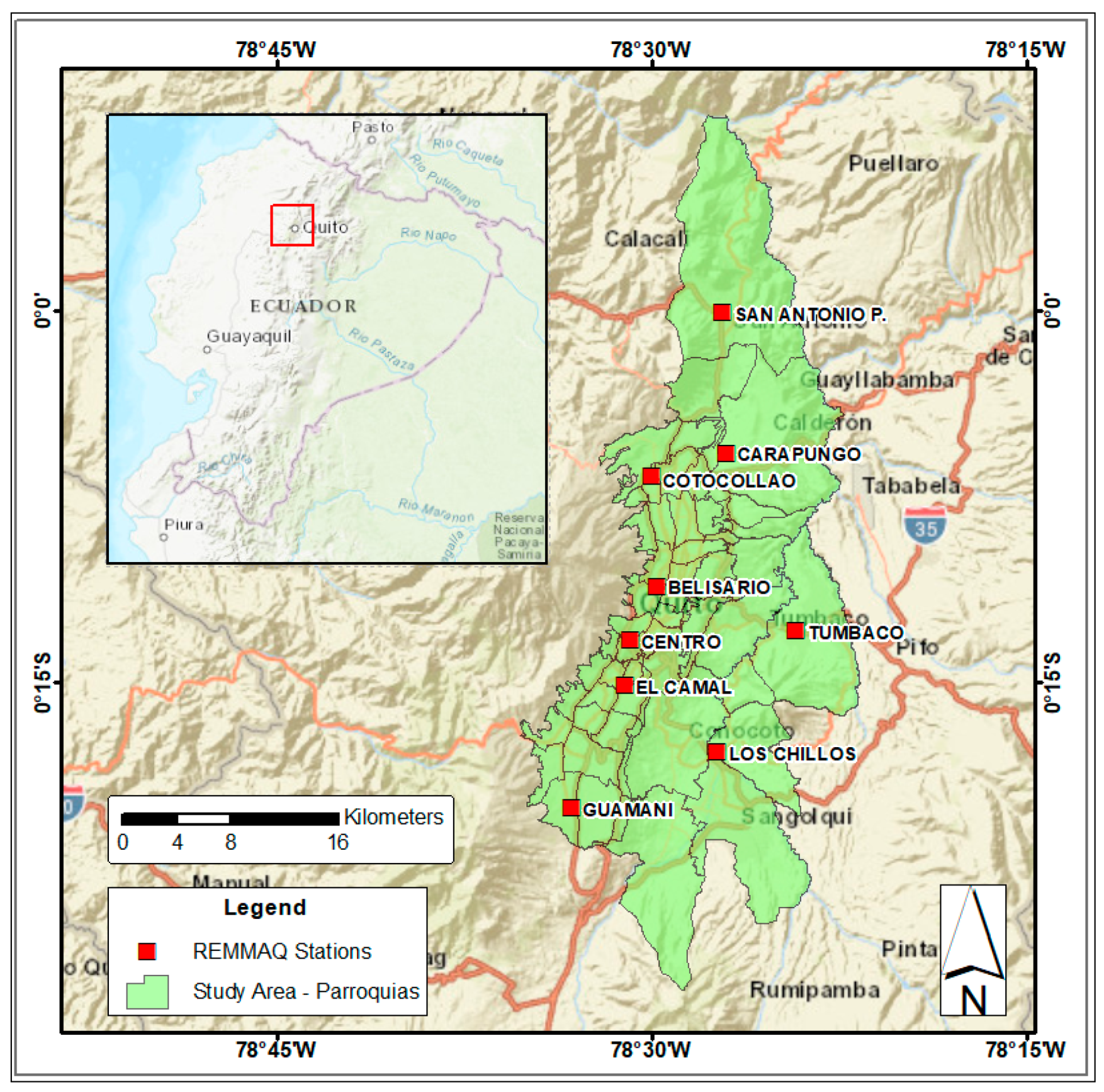
2.1. Study Area
2.2. PM10 Data from AQMN Stations
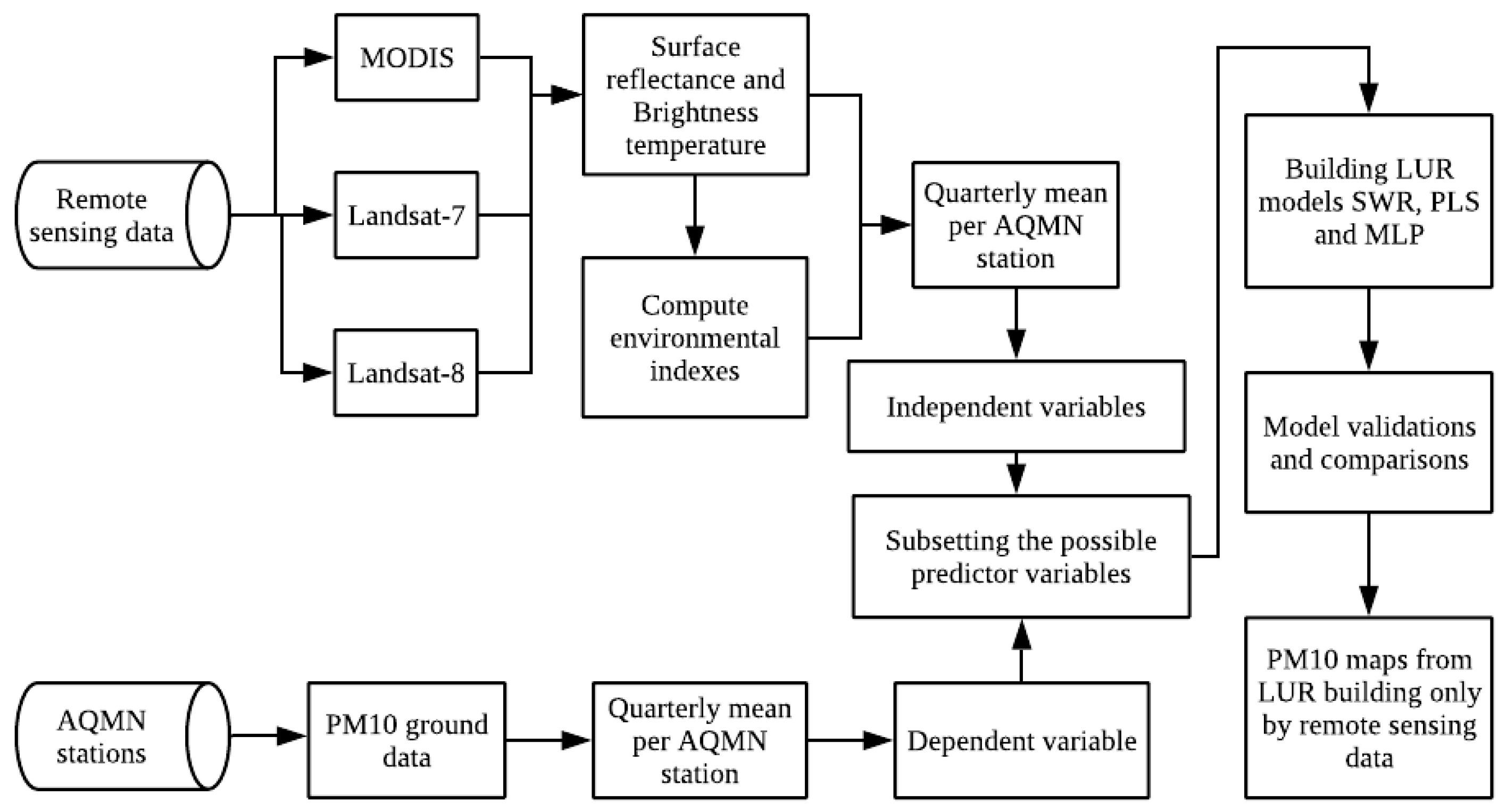
2.3. Remote Sensing Data Predictors
2.4. LUR Models
3. Results
4. Discussion
5. Conclusions
Author Contributions
Acknowledgments
Conflicts of Interest
References
- WHO Ambient (Outdoor) Air Quality and Health. Available online: http://www.who.int/news-room/fact-sheets/detail/ambient-(outdoor)-air-quality-and-health (accessed on 30 August 2018).
- Kutlar Joss, M.; Eeftens, M.; Gintowt, E.; Kappeler, R.; Künzli, N. Time to harmonize national ambient air quality standards. Int. J. Public Health 2017, 62, 453–462. [Google Scholar] [CrossRef] [PubMed] [Green Version]
- Kobza, J.; Geremek, M.; Dul, L. Characteristics of air quality and sources affecting high levels of PM10 and PM2.5 in Poland, Upper Silesia urban area. Environ. Monit. Assess. 2018, 190, 515. [Google Scholar] [CrossRef] [PubMed]
- World Health Organization Regional Office for Europe. Health Effects of Particulate Matter; World Health Organization Regional Office for Europe: København, Denmark, 2013. [Google Scholar]
- Ielpo, P.; Paolillo, V.; de Gennaro, G.; Dambruoso, P.R. PM10 and gaseous pollutants trends from air quality monitoring networks in Bari province: Principal component analysis and absolute principal component scores on a two years and half data set. Chem. Cent. J. 2014, 8, 14. [Google Scholar] [CrossRef] [PubMed]
- Pope, R.; Wu, J. A multi-objective assessment of an air quality monitoring network using environmental, economic, and social indicators and GIS-based models. J. Air Waste Manag. Assoc. 2014, 64, 721–737. [Google Scholar] [CrossRef] [PubMed] [Green Version]
- Capezzuto, L.; Abbamonte, L.; De Vito, S.; Massera, E.; Formisano, F.; Fattoruso, G.; Di Francia, G.; Buonanno, A. A maker friendly mobile and social sensing approach to urban air quality monitoring. In Proceedings of the IEEE SENSORS 2014, Valencia, Spain, 2–5 November 2014; pp. 12–16. [Google Scholar]
- Hasenfratz, D.; Saukh, O.; Walser, C.; Hueglin, C.; Fierz, M.; Thiele, L. Pushing the spatio-temporal resolution limit of urban air pollution maps. In Proceedings of the 2014 IEEE International Conference on Pervasive Computing and Communications (PerCom), Budapest, Hungary, 24–28 March 2014; pp. 69–77. [Google Scholar]
- Alvarez, C.I.; Padilla Almeida, O.; Álvarez Mendoza, C.I.; Padilla Almeida, O. Estimación de la contaminación del aire por PM10 en Quito a través de índices ambientales con imágenes LANDSAT ETM+. Rev. Cart 2016, 135–147. [Google Scholar]
- Cevallos, V.M.; Díaz, V.; Sirois, C.M. Particulate matter air pollution from the city of Quito, Ecuador, activates inflammatory signaling pathways in vitro. Innate Immun. 2017, 23, 392–400. [Google Scholar] [CrossRef] [PubMed] [Green Version]
- Raysoni, A.U.; Armijos, R.X.; Weigel, M.M.; Montoya, T.; Eschanique, P.; Racines, M.; Li, W.-W. Assessment of indoor and outdoor PM species at schools and residences in a high-altitude Ecuadorian urban center. Environ. Pollut. 2016, 214, 668–679. [Google Scholar] [CrossRef] [Green Version]
- Alvarez-Mendoza, C.I.; Teodoro, A.; Torres, N.; Vivanco, V.; Ramirez-Cando, L. Comparison of satellite remote sensing data in the retrieve of PM10 air pollutant over Quito, Ecuador. In Proceedings of the SPIE - The International Society for Optical Engineering, Berlin, Germany, 9 October 2018. [Google Scholar]
- Yang, X.; Zheng, Y.; Geng, G.; Liu, H.; Man, H.; Lv, Z.; He, K.; de Hoogh, K. Development of PM2.5 and NO2 models in a LUR framework incorporating satellite remote sensing and air quality model data in Pearl River Delta region, China. Environ. Pollut. 2017, 226, 143–153. [Google Scholar] [CrossRef]
- Stafoggia, M.; Schwartz, J.; Badaloni, C.; Bellander, T.; Alessandrini, E.; Cattani, G.; de’ Donato, F.; Gaeta, A.; Leone, G.; Lyapustin, A.; et al. Estimation of daily PM10 concentrations in Italy (2006–2012) using finely resolved satellite data, land use variables and meteorology. Environ. Int. 2017, 99, 234–244. [Google Scholar] [CrossRef]
- Shi, Y.; Lau, K.K.-L.; Ng, E. Incorporating wind availability into land use regression modelling of air quality in mountainous high-density urban environment. Environ. Res. 2017, 157, 17–29. [Google Scholar] [CrossRef]
- Son, Y.; Osornio-Vargas, Á.R.; O’Neill, M.S.; Hystad, P.; Texcalac-Sangrador, J.L.; Ohman-Strickland, P.; Meng, Q.; Schwander, S. Land use regression models to assess air pollution exposure in Mexico City using finer spatial and temporal input parameters. Sci. Total Environ. 2018, 639, 40–48. [Google Scholar] [CrossRef]
- Zou, B.; Chen, J.; Zhai, L.; Fang, X.; Zheng, Z.; Zou, B.; Chen, J.; Zhai, L.; Fang, X.; Zheng, Z. Satellite Based Mapping of Ground PM2.5 Concentration Using Generalized Additive Modeling. Remote Sens. 2016, 9, 1. [Google Scholar] [CrossRef]
- Wu, C.-D.; Chen, Y.-C.; Pan, W.-C.; Zeng, Y.-T.; Chen, M.-J.; Guo, Y.L.; Lung, S.-C.C. Land-use regression with long-term satellite-based greenness index and culture-specific sources to model PM2.5 spatial-temporal variability. Environ. Pollut. 2017, 224, 148–157. [Google Scholar] [CrossRef]
- He, J.; Zha, Y.; Zhang, J.; Gao, J. Aerosol indices derived from MODIS data for indicating aerosol-induced air pollution. Remote Sens. 2014, 6, 1587–1604. [Google Scholar] [CrossRef]
- Just, A.; De Carli, M.; Shtein, A.; Dorman, M.; Lyapustin, A.; Kloog, I.; Just, A.C.; De Carli, M.M.; Shtein, A.; Dorman, M.; et al. Correcting Measurement Error in Satellite Aerosol Optical Depth with Machine Learning for Modeling PM2.5 in the Northeastern USA. Remote Sens. 2018, 10, 803. [Google Scholar] [CrossRef]
- Wan, Z. MODIS Land Surface Temperature Products Users’ Guide; Institute for Computational Earth System Science, University of California: Santa Barbara, CA, USA, 2006. [Google Scholar]
- U.S. Geological Survey. Landsat—Earth Observation Satellites; Version 1.; U.S. Geological Survey: Reston, VA, USA, 2015; Volume 2015–3081.
- Olmanson, L.G.; Brezonik, P.L.; Finlay, J.C.; Bauer, M.E. Comparison of Landsat 8 and Landsat 7 for regional measurements of CDOM and water clarity in lakes. Remote Sens. Environ. 2016, 185, 119–128. [Google Scholar] [CrossRef]
- Bilal, M.; Nichol, J.E.; Bleiweiss, M.P.; Dubois, D. A Simplified high resolution MODIS aerosol retrieval algorithm (SARA) for use over mixed surfaces. Remote Sens. Environ. 2013, 136, 135–145. [Google Scholar] [CrossRef]
- Meng, X.; Fu, Q.; Ma, Z.; Chen, L.; Zou, B.; Zhang, Y.; Xue, W.; Wang, J.; Wang, D.; Kan, H.; et al. Estimating ground-level PM10 in a Chinese city by combining satellite data, meteorological information and a land use regression model. Environ. Pollut. 2016, 208, 177–184. [Google Scholar] [CrossRef]
- Shahraiyni, H.T.; Sodoudi, S. Statistical modeling approaches for pm10prediction in urban areas; A review of 21st-century studies. Atmosphere 2016, 7, 15. [Google Scholar] [CrossRef]
- Vermote, E.; Justice, C.; Claverie, M.; Franch, B. Preliminary analysis of the performance of the Landsat 8/OLI land surface reflectance product. Remote Sens. Environ. 2016, 185, 46–56. [Google Scholar] [CrossRef]
- Ayres-Sampaio, D.; Teodoro, A.C.; Sillero, N.; Santos, C.; Fonseca, J.; Freitas, A. An investigation of the environmental determinants of asthma hospitalizations: An applied spatial approach. Appl. Geogr. 2014, 47, 10–19. [Google Scholar] [CrossRef]
- Naughton, O.; Donnelly, A.; Nolan, P.; Pilla, F.; Misstear, B.D.; Broderick, B. A land use regression model for explaining spatial variation in air pollution levels using a wind sector based approach. Sci. Total Environ. 2018, 630, 1324–1334. [Google Scholar] [CrossRef] [Green Version]
- Li, X.; Zhang, Y.; Bao, Y.; Luo, J.; Jin, X.; Xu, X.; Song, X.; Yang, G. Exploring the Best Hyperspectral Features for LAI Estimation Using Partial Least Squares Regression. Remote Sens. 2014, 6, 6221–6241. [Google Scholar] [CrossRef] [Green Version]
- Chen, G.; Meentemeyer, R. Remote Sensing of Forest Damage by Diseases and Insects. In Remote Sensing for Sustainability; Weng, Q., Ed.; Remote Sensing Applications Series; CRC Press: Boca Raton, FL, USA, 2016; p. 357. ISBN 9781315354644. [Google Scholar]
- Xu, W.; Riley, E.A.; Austin, E.; Sasakura, M.; Schaal, L.; Gould, T.R.; Hartin, K.; Simpson, C.D.; Sampson, P.D.; Yost, M.G.; et al. Use of mobile and passive badge air monitoring data for NO X and ozone air pollution spatial exposure prediction models. J. Expo. Sci. Environ. Epidemiol. 2017, 27, 184–192. [Google Scholar] [CrossRef]
- Rosero-Vlasova, O.A.; Vlassova, L.; Pérez-Cabello, F.; Montorio, R.; Nadal-Romero, E. Modeling soil organic matter and texture from satellite data in areas affected by wildfires and cropland abandonment in Aragón, Northern Spain. J. Appl. Remote Sens. 2018, 12, 1. [Google Scholar] [CrossRef]
- Alvarez-Mendoza, C.I.; Teodoro, A.; Ramirez-Cando, L. Spatial estimation of surface ozone concentrations in Quito Ecuador with remote sensing data, air pollution measurements and meteorological variables. Environ. Monit. Assess. 2019, 191, 155. [Google Scholar] [CrossRef]
- Liu, W.; Li, X.; Chen, Z.; Zeng, G.; León, T.; Liang, J.; Huang, G.; Gao, Z.; Jiao, S.; He, X.; et al. Land use regression models coupled with meteorology to model spatial and temporal variability of NO2 and PM10 in Changsha, China. Atmos. Environ. 2015, 116, 272–280. [Google Scholar] [CrossRef]
- Gardner, M.; Dorling, S. Artificial neural networks (the multilayer perceptron)—A review of applications in the atmospheric sciences. Atmos. Environ. 1998, 32, 2627–2636. [Google Scholar] [CrossRef]
- Secretaria del Ambiente de Quito Red Metropolitana de Monitoreo Atmosférico de Quito. Available online: http://www.quitoambiente.gob.ec/ambiente/index.php/generalidades (accessed on 26 June 2018).
- Alvarez, C.I.; Teodoro, A.; Tierra, A. Evaluation of automatic cloud removal method for high elevation areas in Landsat 8 OLI images to improve environmental indexes computation. In Proceedings of the SPIE 10428, Earth Resources and Environmental Remote Sensing/GIS Applications VIII 1042809, Warsaw, Poland, 5 October 2017; Volume 10428, pp. 1042809–1042812. [Google Scholar]
- Alvarez-Mendoza, C.I.; Teodoro, A.; Ramirez-Cando, L. Improving NDVI by removing cirrus clouds with optical remote sensing data from Landsat-8—A case study in Quito, Ecuador. Remote Sens. Appl. Soc. Environ. 2019, 13, 257–274. [Google Scholar] [CrossRef]
- Othman, N.; Jafri, M.Z.M.; San, L.H. Estimating particulate matter concentration over arid region using satellite remote sensing: A case study in Makkah, Saudi Arabia. Mod. Appl. Sci. 2010, 4, 131. [Google Scholar] [CrossRef]
- Bilguunmaa, M.; Batbayar, J.; Tuya, S. Estimation of PM10 concentration using satellite data in Ulaanbaatar City. SPIE Asia Pac. Remote Sens. 2014, 92591O. [Google Scholar] [CrossRef]
- Ángel, M.; Gutiérrez, R. Uso de Modelos Lineales Generalizados (MLG) para la interpolación espacial de PM10 utilizando imágenes satelitales Landsat para la ciudad de Bogotá, Colombia. Perspectiva Geográfica. 2017, 22, 105–121. [Google Scholar] [CrossRef]
- Lee, J.H.; Ryu, J.E.; Chung, H.I.; Choi, Y.Y.; Jeon, S.W.; Kim, S.H. Development of spatial scaling technique of forest health sample point information. In Proceedings of the International Archives of the Photogrammetry, Remote Sensing and Spatial Information Sciences—ISPRS Archives, Beijing, China, 30 April 2018; Volume 42, pp. 751–756. [Google Scholar]
- Ghaleb, F.; Mario, M.; Sandra, A. Regional Landsat-Based Drought Monitoring from 1982 to 2014. Climate 2015, 3, 563–577. [Google Scholar] [CrossRef] [Green Version]
- Sobrino, J.A.; Jiménez-Muñoz, J.C.; Sòria, G.; Romaguera, M.; Guanter, L.; Moreno, J.; Plaza, A.; Martínez, P. Land surface emissivity retrieval from different VNIR and TIR sensors. IEEE Trans. Geosci. Remote Sens. 2008, 46, 316–327. [Google Scholar] [CrossRef]
- Li, S.; Jiang, G.M. Land Surface Temperature Retrieval from Landsat-8 Data with the Generalized Split-Window Algorithm. IEEE Access 2018, 6, 18149–18162. [Google Scholar] [CrossRef]
- Habermann, M.; Billger, M.; Haeger-Eugensson, M. Land use Regression as Method to Model Air Pollution. Previous Results for Gothenburg/Sweden. Procedia Eng. 2015, 115, 21–28. [Google Scholar] [CrossRef] [Green Version]
- Zhang, J.J.Y.; Sun, L.; Barrett, O.; Bertazzon, S.; Underwood, F.E.; Johnson, M. Development of land-use regression models for metals associated with airborne particulate matter in a North American city. Atmos. Environ. 2015, 106, 165–177. [Google Scholar] [CrossRef]
- Williams, L.J.; Abdi, H.; Williams, L.J. Partial Least Squares Methods: Partial Least Squares Correlation and Partial Least Square Regression. In Computational Toxicology: Volume II.; Reisfeld, B., Mayeno, A.N., Eds.; Humana Press: Totowa, NJ, USA, 2013; Volume 930, pp. 549–579. ISBN 978-1-62703-059-5. [Google Scholar]
- Sheela, K.G.; Deepa, S.N. Review on Methods to Fix Number of Hidden Neurons in Neural Networks. Math. Probl. Eng. 2013, 2013, 1–11. [Google Scholar] [CrossRef] [Green Version]
- Cattani, G.; Gaeta, A.; Di Menno di Bucchianico, A.; De Santis, A.; Gaddi, R.; Cusano, M.; Ancona, C.; Badaloni, C.; Forastiere, F.; Gariazzo, C.; et al. Development of land-use regression models for exposure assessment to ultrafine particles in Rome, Italy. Atmos. Environ. 2017, 156, 52–60. [Google Scholar] [CrossRef]
- Wang, M.; Sampson, P.D.; Hu, J.; Kleeman, M.; Keller, J.P.; Olives, C.; Szpiro, A.A.; Vedal, S.; Kaufman, J.D. Combining Land-Use Regression and Chemical Transport Modeling in a Spatiotemporal Geostatistical Model for Ozone and PM 2.5. Environ. Sci. Technol. 2016, 50, 5111–5118. [Google Scholar] [CrossRef]
- Alexeeff, S.E.; Schwartz, J.; Kloog, I.; Chudnovsky, A.; Koutrakis, P.; Coull, B.A. Consequences of kriging and land use regression for PM2.5 predictions in epidemiologic analyses: Insights into spatial variability using high-resolution satellite data. J. Expo. Sci. Environ. Epidemiol. 2015, 25, 138–144. [Google Scholar] [CrossRef]
- Beloconi, A.; Chrysoulakis, N.; Lyapustin, A.; Utzinger, J.; Vounatsou, P. Bayesian geostatistical modelling of PM10 and PM2.5 surface level concentrations in Europe using high-resolution satellite-derived products. Environ. Int. 2018, 121, 57–70. [Google Scholar] [CrossRef]
- Remer, L.A.; Mattoo, S.; Levy, R.C.; Munchak, L.A. MODIS 3 km aerosol product: Algorithm and global perspective. Atmos. Meas. Tech. 2013, 6, 1829–1844. [Google Scholar] [CrossRef]
- Teodoro, A. A study on the Quality of the Vegetation Index obtainded from MODIS Data. In Proceedings of the 2015 IEEE International Geoscience and Remote Sensing Symposium, Milan, Italy, 26–31 July 2015; pp. 3365–3368. [Google Scholar]
- Saucy, A.; Röösli, M.; Künzli, N.; Tsai, M.Y.; Sieber, C.; Olaniyan, T.; Baatjies, R.; Jeebhay, M.; Davey, M.; Flückiger, B.; et al. Land use regression modelling of outdoor NO2 and PM2.5 concentrations in three low income areas in the western cape province, South Africa. Int. J. Environ. Res. Public Health 2018, 15, 1452. [Google Scholar] [CrossRef]
- Lv, Y.; Liu, J.; Yang, T. Nonlinear PLS Integrated with Error-Based LSSVM and Its Application to NO2 Modeling. Ind. Eng. Chem. Res. 2012, 51, 16092–16100. [Google Scholar] [CrossRef]
- Secretaria del Ambiente de Quito. IAMQ/18; Secretaria del Ambiente de Quito: Quito, Ecuador, 2018.
- Romero, D.; El parque automotor aumenta y complica más la movilidad. El Comer. 2017, 1. Available online: https://www.elcomercio.com/actualidad/aumento-parque-automotor-quito-movilidad.html (accessed on 13 June 2019).
- Todoroski Air Sciences. Air Quality Impact Assessment Sandy Point Quarry Epl Variation; Todoroski Air Sciences: Eastwood, Australia, 2019. [Google Scholar]


| Satellite | Sensor | Overpass Time of Satellite | Spatial Resolution |
|---|---|---|---|
| Landsat-7 | Enhanced Thematic Mapper Plus (ETM+) | 16 days | 30 m |
| Landsat-8 | Operational Land Imager (OLI) Thermal Infrared Sensor (TIRS) | 16 days | 30 m |
| Terra (EOS AM-1) Aqua (EOS PM-1) | Moderate Resolution Imaging Spectroradiometer (MODIS) MCD43A4 | 1 to 2 days | 500 m |
| Predictors | Landsat-7 | Landsat-8 | MODIS |
|---|---|---|---|
| Blue band (B) Green band (G) Red band (R) Near Infrared (NIR) Short Wave infrared (SWIR) | Landsat surface data Level-2 | Landsat surface data Level-2 | MODIS MOD09A1 MYD09A1 products |
| Normalized Difference Vegetation Index (NDVI) | (1) | MODIS MOD13Q1 MYD13Q1products | |
| Normalized Difference Soil Index (NDSI) | (2) | ||
| Soil-Adjusted Vegetation Index (SAVI) | (3) where L represents a minimal change in the soil brightness with a value of 0.5 [43] | ||
| Normalized Difference Water Index (NDWI) | (4) | ||
| Land Surface Temperature (LST) | (5) where BT is the brightness temperature, λ is the center wavelength (Landsat-7 = 11.45 μm, Landsat-8 = 10.8 μm) [44], is a constant and ε is the emissivity [45,46]. | MODIS MOD11A1 MYD11A1 products | |
| Variable | Landsat-7 | Landsat-8 | MODIS |
|---|---|---|---|
| No. Observations | 35 | 93 | 108 |
| No. Predictors | 5 | 8 | 6 |
| Predictors | NDVI B R NIR S | NDVI SAVI LST B G R NIR Y | NDVI B G R NIR S |
| Sensor | Model | Equation/Method | Coefficient of Determination (R2) | Root-Mean-Square Error (RMSE) |
|---|---|---|---|---|
| Landsat-7 ETM+ | Stepwise regression (STW) | (7) | 0.37 | 9.47 |
| Partial least square regression (PLS) | (8) | 0.36 | 10.14 | |
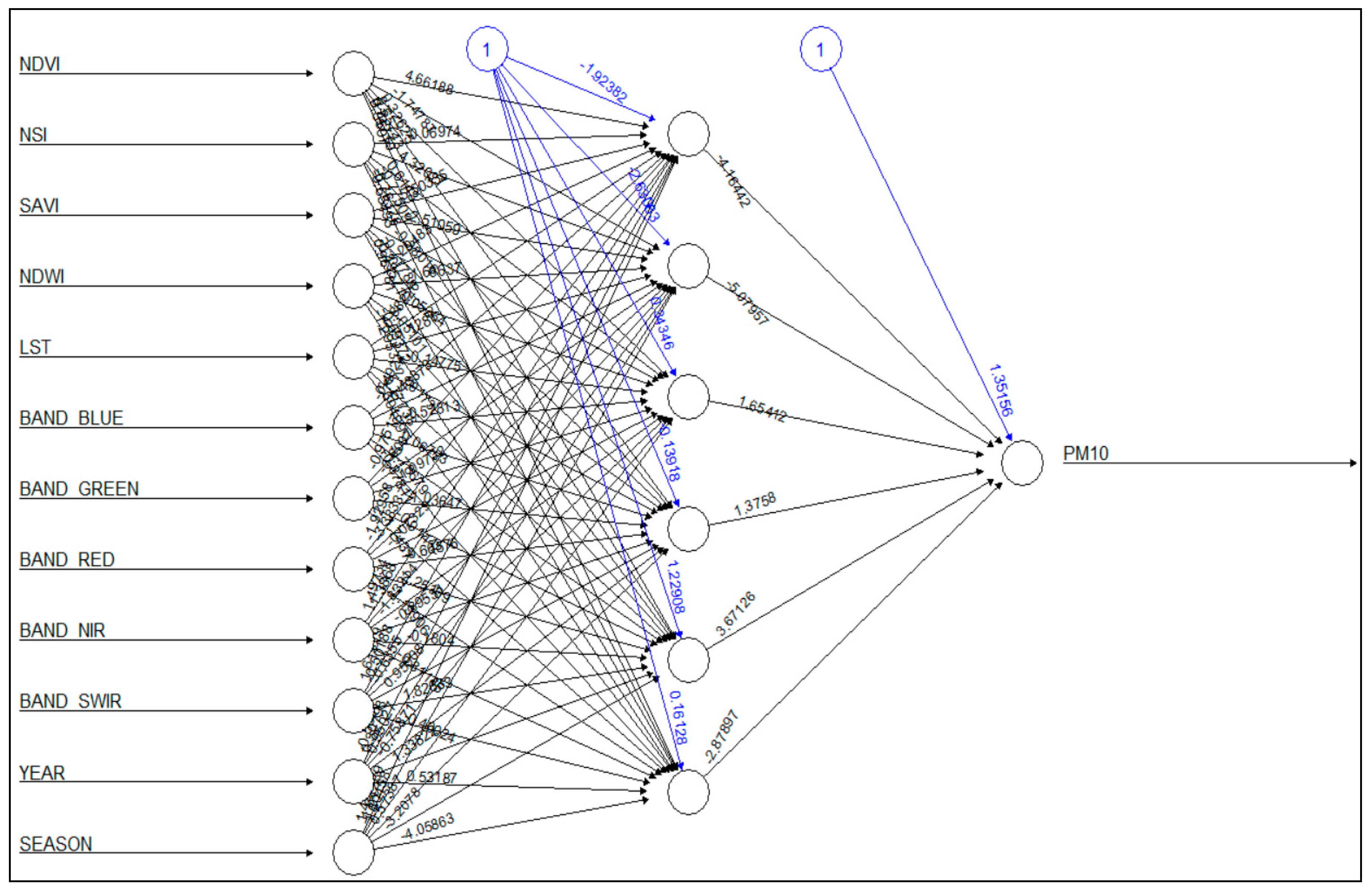
| Multilayer perceptron (MLP) | Non-linear. One hidden layer and six hidden nodes. | 0.46 | 12.69 | |
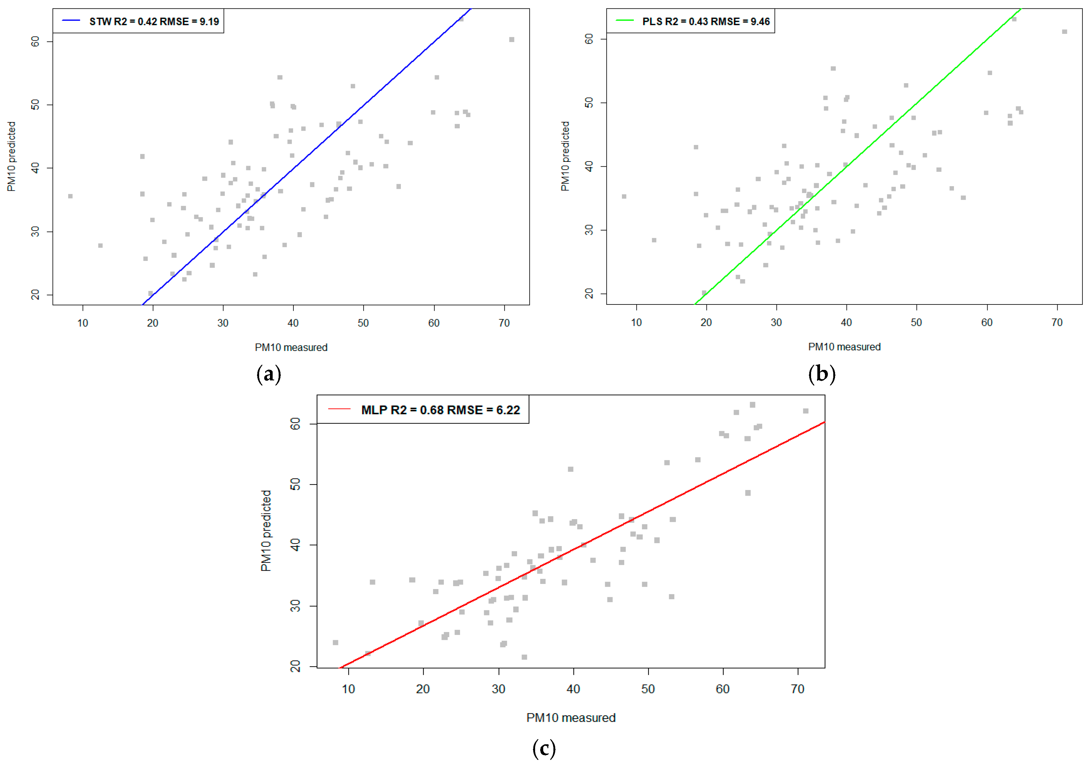
| Landsat-8 OLI/TIRS | STW | (9) | 0.42 | 9.19 |
| PLS | (10) | 0.43 | 9.46 | |
| MLP | Non-linear. One hidden layer and six hidden nodes. | 0.68 | 6.22 | |
| MODIS | STW | (11) | 0.15 | 12.91 |
| PLS | (12) | 0.19 | 12.93 | |
| MLP | Non-linear. One hidden layer and six hidden nodes. | 0.25 | 16.38 |
© 2019 by the authors. Licensee MDPI, Basel, Switzerland. This article is an open access article distributed under the terms and conditions of the Creative Commons Attribution (CC BY) license (http://creativecommons.org/licenses/by/4.0/).
Share and Cite
Alvarez-Mendoza, C.I.; Teodoro, A.C.; Torres, N.; Vivanco, V. Assessment of Remote Sensing Data to Model PM10 Estimation in Cities with a Low Number of Air Quality Stations: A Case of Study in Quito, Ecuador. Environments 2019, 6, 85. https://0-doi-org.brum.beds.ac.uk/10.3390/environments6070085
Alvarez-Mendoza CI, Teodoro AC, Torres N, Vivanco V. Assessment of Remote Sensing Data to Model PM10 Estimation in Cities with a Low Number of Air Quality Stations: A Case of Study in Quito, Ecuador. Environments. 2019; 6(7):85. https://0-doi-org.brum.beds.ac.uk/10.3390/environments6070085
Chicago/Turabian StyleAlvarez-Mendoza, Cesar I., Ana Claudia Teodoro, Nelly Torres, and Valeria Vivanco. 2019. "Assessment of Remote Sensing Data to Model PM10 Estimation in Cities with a Low Number of Air Quality Stations: A Case of Study in Quito, Ecuador" Environments 6, no. 7: 85. https://0-doi-org.brum.beds.ac.uk/10.3390/environments6070085