Is a Land Use Regression Model Capable of Predicting the Cleanest Route to School?

 , ,
, , 

Abstract
:1. Introduction
2. Materials and Methods
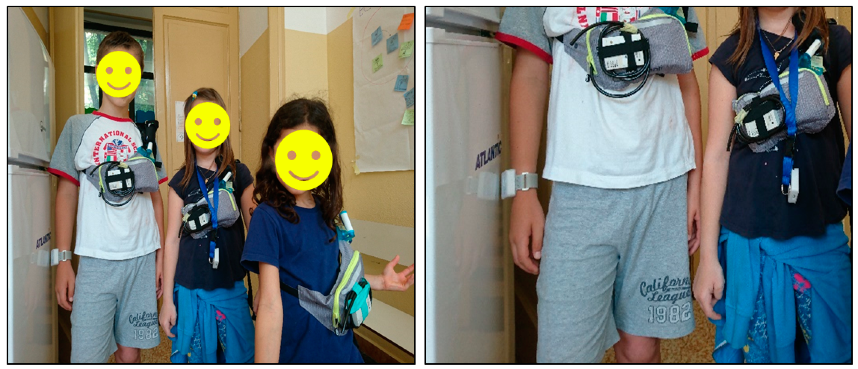
2.1. Study Design
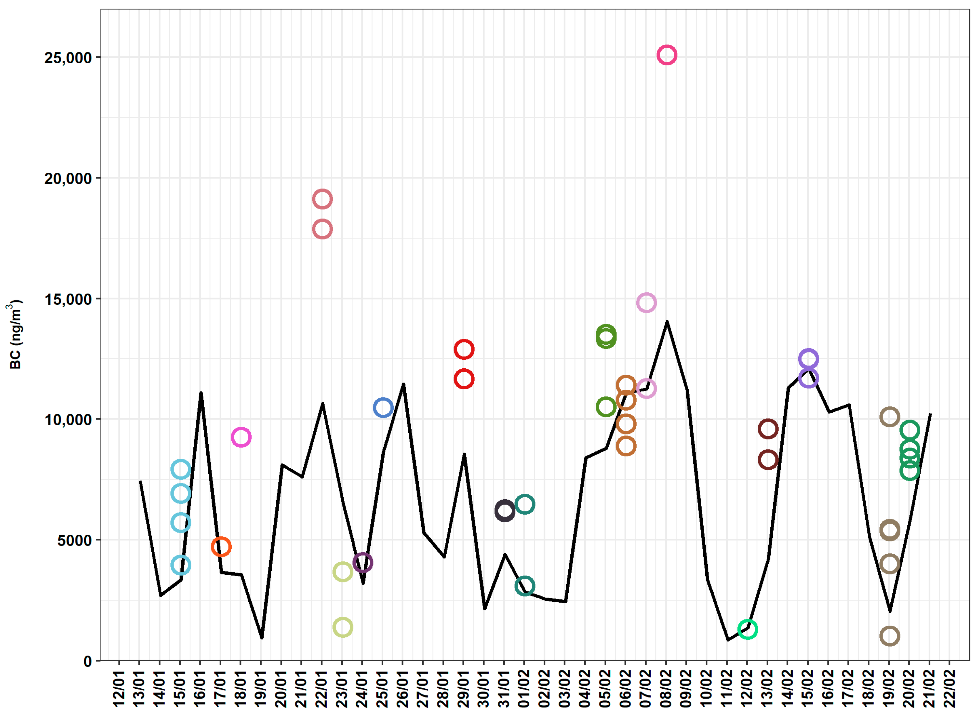
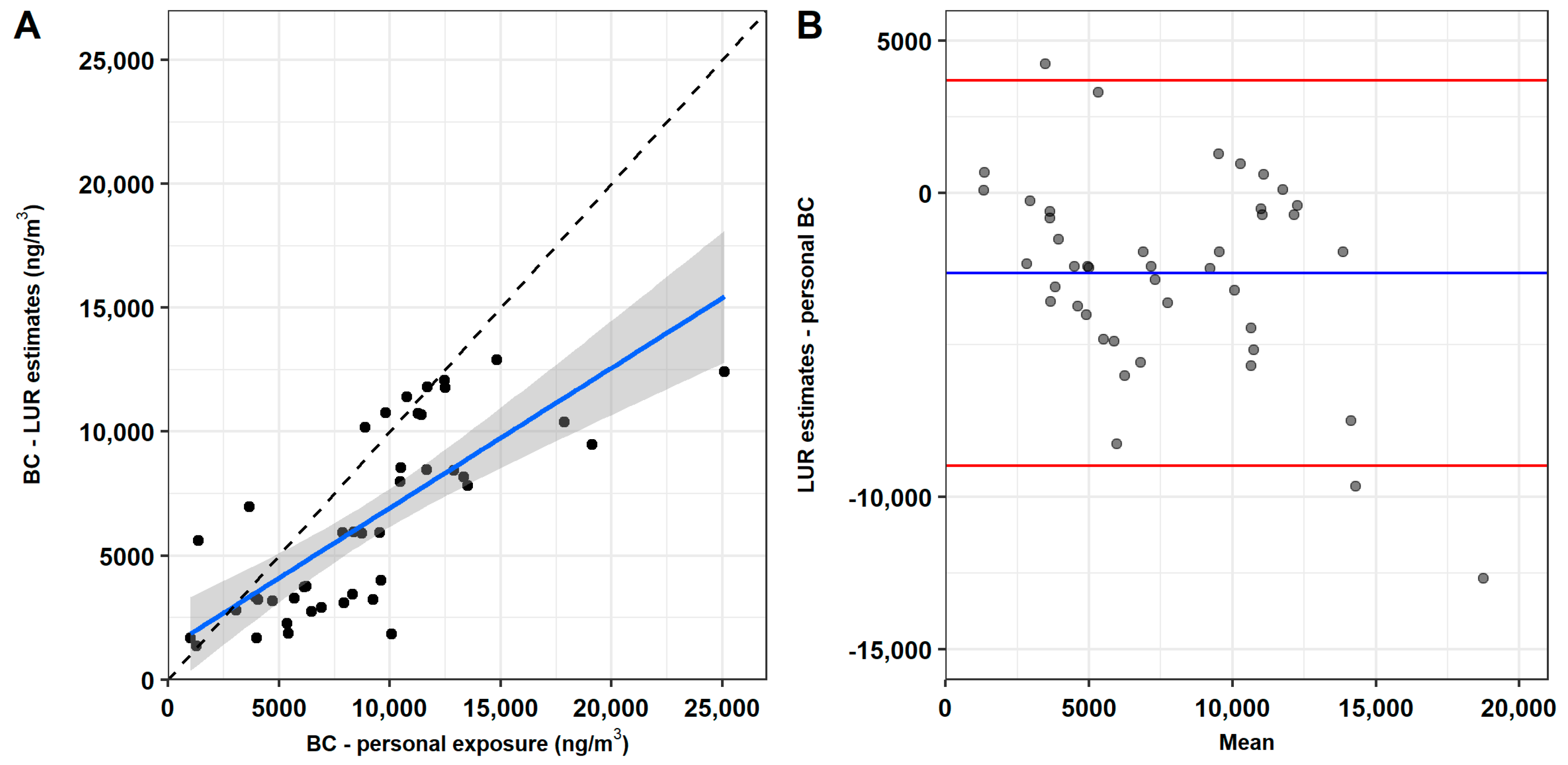
2.2. Data Analysis
3. Results
4. Discussion
5. Conclusions
Author Contributions
Funding
Acknowledgments
Conflicts of Interest
References
- Ryan, P.H.; LeMasters, G.K. A review of land-use regression models for characterizing intraurban air pollution exposure. Inhal. Toxicol. 2007, 19 (Suppl. 1), 127–133. [Google Scholar] [CrossRef] [PubMed]
- Hoek, G.; Beelen, R.; de Hoogh, K.; Vienneau, D.; Gulliver, J.; Fischer, P.; Briggs, D. A review of land-use regression models to assess spatial variation of outdoor air pollution. Atmos. Environ. 2008, 42, 7561–7578. [Google Scholar] [CrossRef]
- Dias, D.; Tchepel, O. Spatial and Temporal Dynamics in Air Pollution Exposure Assessmen. Int. J. Environ. Res. Public Health 2018, 15, 558. [Google Scholar] [CrossRef] [PubMed]
- Dons, E.; Laeremans, M.; Orjuela, J.P.; Palencia, I.A.; de Nazelled, A.; Nieuwenhuijsen, M.; Van Poppel, M.; Carrasco-Turigase, G.; Standaert, A.; De Boever, P.; et al. Transport most likely to cause air pollution peak exposures in everyday life: Evidence from over 2000 days of personal monitoring. Atmos. Environ. 2009, 213, 424–432. [Google Scholar] [CrossRef]
- Dons, E.; Int Panis, L.; Van Poppel, M.; Theunis, J.; Wets, G. Personal exposure to Black Carbon in transport microenvironments. Atmos. Environ. 2012, 55, 392–398. [Google Scholar] [CrossRef]
- Buonanno, G.; Stabile, L.; Morawska, L.; Russi, A. Children exposure assessment to ultrafine particles and black carbon: The role of transport and cooking activities. Atmos. Environ. 2013, 79, 53–58. [Google Scholar] [CrossRef] [Green Version]
- WHO. Health and environment: Addressing the health impact of air pollution. 2015. Available online: https://apps.who.int/iris/handle/10665/253206 (accessed on 27 July 2019).
- Health Effect Institute (HEI). Understanding the Health Effects of Ambient Ultrafine Particles. 2012. Available online: https://www.healtheffects.org/system/files/Perspectives3.pdf (accessed on 27 July 2019).
- Janssen, N.A.; Hoek, G.; Simic-Lawson, M.; Fischer, P.; van Bree, L.; ten Brink, H.; Keuken, M.; Atkinson, R.W.; Anderson, H.R.; Brunekreef, B.; et al. Black Carbon as an Additional Indicator of the Adverse Health Effects of Airborne Particles Compared with PM10 and PM2.5. Environ. Health Perspect. 2011, 119, 1691–1699. [Google Scholar] [CrossRef]
- WHO. Health effects of Black Carbon. 2012. Available online: http://www.euro.who.int/en/health-topics/environment-and-health/air-quality/publications/2012/health-effects-of-black-carbon-2012 (accessed on 27 July 2019).
- Rivas, I.; Donaire-Gonzalez, D.; Bouso, L.; Esnaola, M.; Pandolfi, M.; de Castro, M.; Viana, M.; Alvarez-Pedrerol, M.; Nieuwenhuijsen, M.; Alastuey, A.; et al. Spatiotemporally resolved black carbon concentration, schoolchildren’s exposure and dose in Barcelona. Indoor Air 2016, 26, 391–402. [Google Scholar] [CrossRef]
- Boniardi, L.; Dons, E.; Campo, L.; Van Poppel, M.; Int Panis, L.; Fustinoni, S. Annual, seasonal, and morning rush hour Land Use Regression models for black carbon in a school catchment area of Milan, Italy. Environ. Res. 2019, 176, 108520. [Google Scholar] [CrossRef]
- Provost, E.B.; Int Panis, L.; Saenen, N.D.; Kicinskia, M.; Louwies, T.; Vrijens, K.; De Boever, P.; Nawrot, T.S. Recent versus chronic fine particulate air pollution exposure as determinant of the retinal microvasculature in school children. Environ. Res. 2017, 159, 103–110. [Google Scholar] [CrossRef]
- Rice, M.B.; Rifas-Shiman, S.L.; Litonjua, A.A.; Oken, E.; Gillman, M.W.; Kloog, I.; Luttmann-Gibson, H.; Zanobetti, A.; Coull, B.A.; Schwartz, J.; et al. Lifetime Exposure to Ambient Pollution and Lung Function in Children. Am. J. Respir. Crit. Care Med. 2016, 193, 881–888. [Google Scholar] [CrossRef] [PubMed] [Green Version]
- Lin, W.; Huang, W.; Zhu, T.; Hu, M.; Brunekreef, B.; Zhang, Y.; Liu, X.; Cheng, H.; Gehring, U.; Li, C.; et al. Acute respiratory inflammation in children and black carbon in ambient air before and during the 2008 Beijing Olympics. Environ. Health Perspect. 2011, 119, 1507–1512. [Google Scholar] [CrossRef] [PubMed]
- Chiu, Y.H.; Bellinger, D.C.; Coull, B.A.; Anderson, S.; Barber, R.; Wright, R.O.; Wright, R.J. Associations between traffic-related black carbon exposure and attention in a prospective birth cohort of urban children. Environ. Health Perspect. 2013, 121, 859–864. [Google Scholar] [CrossRef] [PubMed]
- Guxens, M.; Lubczyńska, M.J.; Muetzel, R.L.; Dalmau-Bueno, A.; Jaddoe, V.W.V.; Hoek, G.; van der Lugt, A.; Verhulst, F.C.; White, T.; Brunekreef, B.; et al. Air Pollution Exposure During Fetal Life, Brain Morphology, and Cognitive Function in School-Age Children. Biol. Psychiatry 2018, 84, 295–303. [Google Scholar] [CrossRef] [PubMed] [Green Version]
- Sunyer, J.; Esnaola, M.; Alvarez-Pedrerol, M.; Forns, J.; Rivas, I.; López-Vicente, M.; Suades-González, E.; Foraster, M.; Garcia-Esteban, R.; Basagaña, X.; et al. Association between traffic-related air pollution in schools and cognitive development in primary school children: A prospective cohort study. PLoS Med. 2015, 12, e1001792. [Google Scholar] [CrossRef] [PubMed]
- Bose, S.; Romero, K.; Psoter, K.J.; Curriero, F.C.; Chen, C.; Johnson, C.M.; Kaji, D.; Breysse, P.N.; Williams, D.L.; Ramanathan, M.; et al. Association of traffic air pollution and rhinitis quality of life in Peruvian children with asthma. PLoS ONE 2018, 13, e0193910. [Google Scholar] [CrossRef] [PubMed]
- Alvarez-Pedrerol, M.; Rivas, I.; López-Vicente, M.; Suades-González, E.; Donaire-Gonzalez, D.; Cirach, M.; de Castro, M.; Esnaola, M.; Basagaña, X.; Dadvand, P.; et al. Impact of commuting exposure to traffic-related air pollution on cognitive development in children walking to school. Environ. Pollut. 2017, 231 Pt 1, 837–844. [Google Scholar] [CrossRef] [PubMed] [Green Version]
- Hankey, S.; Lindsey, G.; Marshall, J.D. Population-Level Exposure to Particulate Air Pollution during Active Travel: Planning for Low-Exposure, Health-Promoting Cities. Environ. Health Perspect. 2017, 125, 527–534. [Google Scholar] [CrossRef]
- Tainio, M.; de Nazelle, A.J.; Götschi, T.; Kahlmeier, S.; Rojas-Rueda, D.; Nieuwenhuijsen, M.J.; de Sá, T.H.; Kelly, P.; Woodcock, J. Can air pollution negate the health benefits of cycling and walking? Prev. Med. 2016, 87, 233–236. [Google Scholar] [CrossRef] [Green Version]
- Mueller, N.; Rojas-Rueda, D.; Basagaña, X.; Cirach, M.; Cole-Hunter, T.; Dadvand, P.; Donaire-Gonzalez, D.; Foraster, M.; Gascon, M.; Martinez, D.; et al. Health impacts related to urban and transport planning: A burden of disease assessment. Environ. Int. 2017, 107, 243–257. [Google Scholar] [CrossRef] [Green Version]
- Khreis, H.; Nieuwenhuijsen, M.J. Traffic-Related Air Pollution and Childhood Asthma: Recent Advances and Remaining Gaps in the Exposure Assessment Methods. Int. J. Environ. Res. Public Health 2017, 14, 312. [Google Scholar] [CrossRef] [PubMed]
- National Statistics Institute (ISTAT). 2018. Available online: http://dati.istat.it/Index.aspx?DataSetCode=DCIS_POPRES1 (accessed on 27 July 2019).
- Weingartner, E.; Saatho, H.; Schnaiterb, M.; Streita, N.; Bitnarc, B.; Baltensperger, U. Absorption of light by soot particles: Determination of the absorption coefficient by means of aethalometers. J. Aerosol. Sci. 2003, 34, 1445–1463. [Google Scholar] [CrossRef]
- Good, N.; Molter, A.; Peel, J.L.; Volckens, J. An accurate filter loading correction is essential for assessing personal exposure to black carbon using an Aethalometer. J. Expo. Sci. Environ. Epidemiol. 2017, 27, 409–416. [Google Scholar] [CrossRef] [PubMed]
- Hagler, G.S.W.; Yelverton, T.L.B.; Vedantham, R.; Hansen, A.D.A.; Turner, J.D. Post-processing method to reduce noise while preserving high time resolution in Aethalometer real-time black carbon data. Aerosol. Air Qual. Res. 2011, 11, 539–546. [Google Scholar] [CrossRef]
- Virkkula, A.; Mäkelä, T.; Hillamo, R.; Yli-Tuomi, T.; Hirsikko, A.; Hämeri, K.; Koponen, I.K. A simple procedure for correcting loading effects of aethalometer data. J. Air Waste Manag. Assoc. 2007, 57, 1214–1222. [Google Scholar] [CrossRef] [PubMed]
- Eeftens, M.; Beelen, R.; de Hoogh, K.; Bellander, T.; Cesaroni, G.; Cirach, M.; Declercq, C.; Dėdelė, A.; Dons, E.; de Nazelle, A.; et al. Development of Land Use Regression Models for PM2.5, PM2.5 absorbance, PM10 and Pmcoarse in 20 European Study Areas; Results of the Escape Project. Environ. Sci. Technol. 2012, 46, 11195–11205. [Google Scholar] [CrossRef] [PubMed]
- QGIS Development Team. QGIS Geographic Information System. Open Source Geospatial Foundation Project. 2016. Available online: http://qgis.osgeo.org (accessed on 27 July 2019).
- Henderson, S.B.; Beckerman, B.; Jerrett, M.; Brauer, M. Application of land use regression to estimate long-term concentrations of traffic-related nitrogen oxides and fine particulate matter. Environ. Sci. Technol. 2007, 41, 2422–2428. [Google Scholar] [CrossRef]
- R Core Team. R: A Language and Environment for Statistical Computing; R Foundation for Statistical Computing: Vienna, Austria, 2014; Available online: http://www.R-project.org/ (accessed on 27 July 2019).
- Nieuwenhuijsen, M.J.; Donaire-Gonzalez, D.; Rivas, I.; de Castro, M.; Cirach, M.; Hoek, G.; Seto, E.; Jerrett, M.; Sunyer, J. Variability in and agreement between modeled and personal continuously measured black carbon levels using novel smartphone and sensor technologies. Environ. Sci. Technol. 2015, 49, 2977–2982. [Google Scholar] [CrossRef]
- Paunescu, A.C.; Attoui, M.; Bouallala, S.; Sunyer, J.; Momas, I. Personal measurement of exposure to black carbon and ultrafine particles in schoolchildren from PARIS cohort (Paris, France). Indoor Air 2017, 27, 766–779. [Google Scholar] [CrossRef]
- Cunha-Lopes, I.; Martins, V.; Faria, T.; Correia, C.; Almeida, S.M. Children’s exposure to sized-fractioned particulate matter and black carbon in an urban environment. Build. Environ. 2019, 155, 187–194. [Google Scholar] [CrossRef]
- Minet, L.; Liu, R.; Valois, M.F.; Xu, J.; Weichenthal, S.; Hatzopoulou, M. Development and Comparison of Air Pollution Exposure Surfaces Derived from On-Road Mobile Monitoring and Short-Term Stationary Sidewalk Measurements. Environ. Sci. Technol. 2018, 52, 3512–3519. [Google Scholar] [CrossRef] [PubMed]
- Van Nunen, E.; Vermeulen, R.; Tsai, M.Y.; Probst-Hensch, N.; Ineichen, A.; Davey, M.; Imboden, M.; Ducret-Stich, R.; Naccarati, A.; Raffaele, D.; et al. Land Use Regression Models for Ultrafine Particles in Six European Areas. Environ. Sci. Technol. 2017, 51, 3336–3345. [Google Scholar] [CrossRef] [PubMed] [Green Version]
- Tunno, B.J. Spatial Patterns in Rush-Hour vs. Work-Week Diesel-Related Pollution across a Downtown CoreInt. J. Environ. Res. Public Health 2018, 15, 1968. [Google Scholar] [CrossRef] [PubMed]
- Anowar, S.; Eluru, N.; Hatzopoulou, M. Quantifying the value of a clean ride: How far would you bicycle to avoid exposure to traffic-related air pollution? Transp. Res. Part A 2017, 105, 66–78. [Google Scholar] [CrossRef]


| Mean ± SD | Min–Max | |
|---|---|---|
| Age (years) | 9.1 ± 0.7 | 7–11 |
| Distance (m) | 650 ± 258 | 114–1403 |
| Measured BC (ng/m3) | 9003 ± 4864 | 1014–25,097 |
| MRH LUR BC estimate (ng/m3) | 6365 ± 3676 | 1365–12,886 |
| MRH AQN background BC (ng/m3) | 6635 ± 3730 | 1350–14,050 |
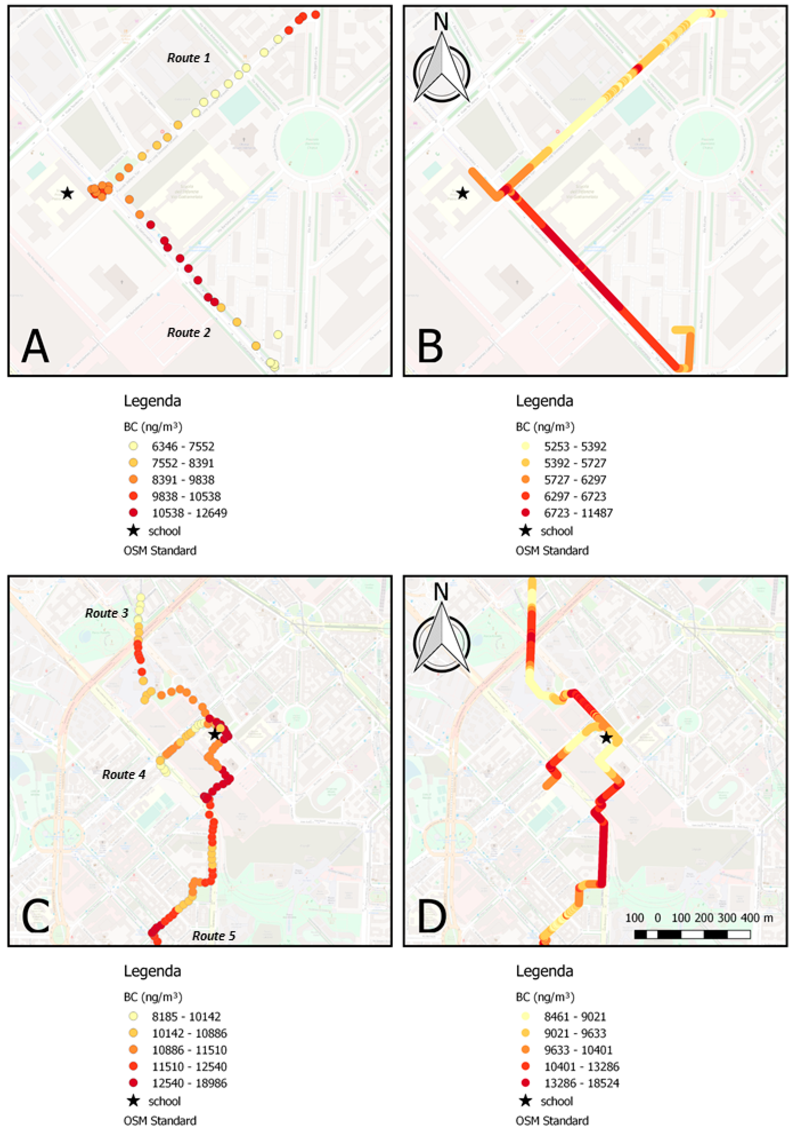
| Route | Day | Distance (m) | Measured BC (Mean ± SD, ng/m3) | MRH LUR BC Estimate (Mean ± SD, ng/m3) | MRH AQN Background BC (Mean, ng/m3) |
|---|---|---|---|---|---|
| Route 1 | 13/02/2019 | 482 | 8320 ± 1892 | 5633 ± 761 | 4200 |
| Route 2 | 13/02/2019 | 486 | 9591 ± 2189 | 6576 ± 871 | 4200 |
| Route 3 | 06/02/2019 | 939 | 9798 ± 2217 | 10,753 ± 2510 | 11,100 |
| Route 4 | 06/02/2019 | 492 | 8884 ± 2125 | 10,169 ± 1954 | 11,100 |
| Route 5 | 06/02/2019 | 1403 | 10,779 ± 4594 | 11,390 ± 2490 | 11,100 |
© 2019 by the authors. Licensee MDPI, Basel, Switzerland. This article is an open access article distributed under the terms and conditions of the Creative Commons Attribution (CC BY) license (http://creativecommons.org/licenses/by/4.0/).
Share and Cite
Boniardi, L.; Dons, E.; Campo, L.; Van Poppel, M.; Int Panis, L.; Fustinoni, S. Is a Land Use Regression Model Capable of Predicting the Cleanest Route to School? Environments 2019, 6, 90. https://0-doi-org.brum.beds.ac.uk/10.3390/environments6080090
Boniardi L, Dons E, Campo L, Van Poppel M, Int Panis L, Fustinoni S. Is a Land Use Regression Model Capable of Predicting the Cleanest Route to School? Environments. 2019; 6(8):90. https://0-doi-org.brum.beds.ac.uk/10.3390/environments6080090
Chicago/Turabian StyleBoniardi, Luca, Evi Dons, Laura Campo, Martine Van Poppel, Luc Int Panis, and Silvia Fustinoni. 2019. "Is a Land Use Regression Model Capable of Predicting the Cleanest Route to School?" Environments 6, no. 8: 90. https://0-doi-org.brum.beds.ac.uk/10.3390/environments6080090