
Multi-Year Monitoring of Ecosystem Metabolism in Two Branches of a Cold-Water Stream


Department of Environmental Studies, Macalester College, St. Paul, MN 55113, USA
Environments 2021, 8(3), 19; https://0-doi-org.brum.beds.ac.uk/10.3390/environments8030019
Submission received: 26 January 2021
/
Revised: 23 February 2021
/
Accepted: 24 February 2021
/
Published: 28 February 2021
(This article belongs to the Special Issue Monitoring and Management of Inland Waters)
Abstract
:Climate change is likely to have large impacts on freshwater biodiversity and ecosystem function, especially in cold-water streams. Ecosystem metabolism is affected by water temperature and discharge, both of which are expected to be affected by climate change and, thus, require long-term monitoring to assess alterations in stream function. This study examined ecosystem metabolism in two branches of a trout stream in Minnesota, USA over 3 years. One branch was warmer, allowing the examination of elevated temperature on metabolism. Dissolved oxygen levels were assessed every 10 min from spring through fall in 2017–2019. Gross primary production (GPP) was higher in the colder branch in all years. GPP in both branches was highest before leaf-out in the spring. Ecosystem respiration (ER) was greater in the warmer stream in two of three years. Both streams were heterotrophic in all years (net ecosystem production—NEP < 0). There were significant effects of temperature and light on GPP, ER, and NEP. Stream discharge had a significant impact on all GPP, ER, and NEP in the colder stream, but only on ER and NEP in the warmer stream. This study indicated that the impacts of temperature, light, and discharge differ among years, and, at least at the local scale, may not follow expected patterns.
1. Introduction
Freshwater biodiversity and ecosystem function are vulnerable to climate change [1,2,3,4]. The major impacts of climate change on stream systems are likely to cause alterations in water temperature, light regime due to shifting phenological patterns in watersheds, and hydrological function because of changing precipitation patterns [5]. These changes are projected to have impacts on water quality [6,7,8] and are expected to influence individual organisms, populations, and communities [9], substantially impacting food webs [10]. Since their value in providing ecosystem services (such as nutrient cycling, water purification, carbon sequestration, and recreational opportunities) and the impacts that climate change may have on these resources, there must be long-term monitoring of these systems [11].
Climate change is especially likely to have major effects on cold-water streams [12], with the impact depending on the spatial scale examined [13]. Warming temperatures in cold-water streams may influence stenothermal organisms that often occupy these habitats, potentially resulting in their replacement with more thermally tolerant species [14,15]. There is a particular concern about the potential loss of cold-water fish species because of their importance for recreational and commercial fisheries [16,17,18,19,20]. While many cold-water systems are fed by groundwater, climate change may result in increasing groundwater temperatures or a decline in groundwater input leading to increasing stream temperatures [21,22,23].
Ecosystem metabolism measures the collective metabolic activity of all of the organisms in an ecosystem [24,25]. In stream systems, ecosystem metabolism is most often based on changes in the oxygen content of the water related to two metabolic processes: photosynthesis and respiration [26,27,28]. Young et al. [29] provide a series of expected changes to ecosystem metabolism to a range of environmental stressors such as toxic chemicals, channelization and nutrient enrichment, and natural variation. Bernhardt et al. [5] provided an overview of the drivers of ecosystem metabolism, including light, heat, allochthonous inputs, and hydrologic disturbance, and developed a set of recommendations for additional research necessary to better characterize these drivers. Since ecosystem metabolism varies with differences in annual climatic patterns, climate change is also likely to influence stream metabolism [30]. Staehr et al. [31] reviewed how climate change could influence aquatic ecosystem metabolism. They suggested that new and more affordable instrumentation will increase our understanding of how processes such as climate change and management actions influence ecosystem metabolism.
Using ecosystem metabolism in streams has been suggested as a measure of ecosystem health, since it can be influenced by pollution, eutrophication, alterations of the physical stream habitat, drought, salinization, acidification, and land use [32,33,34]. For example, Huang et al. [35] indicated that ecosystem metabolism could be used as a means to measure the response of rivers to changes in minimum environmental flows. Human land use can influence both the level and variability of stream metabolism [36], and stream metabolism has been used to compare agricultural catchments employing different best management practices [37]. Several studies have suggested using stream metabolism measures to better manage stream ecosystems [5,30,38].
The components of ecosystem metabolism include gross primary production (GPP), ecosystem respiration (ER), and the balance between these, net ecosystem production (NEP). GPP and ER play a significant role in organic carbon fluxes in stream systems [39]. Warming temperatures associated with climate change are likely to result in streams becoming more heterotrophic and contributing more CO2 to the atmosphere [40,41]. Even though small streams have relatively low GPP, they can disproportionately affect the GPP of a river network because of their large overall surface area [42].
Despite the potential usefulness of using measures of ecosystem metabolism to track the impact of climate change on streams, few studies have looked at interannual variability, which is necessary to track long-term trends in warming. Large river systems can have substantial interannual variation in measures of ecosystem metabolism, often related to stochastic events, although seasonal variation can account for about half of the total variation [43]. In headwater streams, interannual variability also seems to be controlled mainly by local stochastic events (storm frequency and macroalgal blooms) or global events (El Niño—Southern Oscillation) [44,45]. Interannual variability can also be influenced by varying human land use over time, and thus, long-term temporal monitoring is required to assess how streams respond to changes in both natural and human impacts [36].
In this study, ecosystem metabolism was assessed in two branches of a cold-water stream. Metabolism in these locations was studied in the fall of 2015 by Hornbach et al. [46]. One location was generally colder than the other but unexpectedly had higher GPP. While this location had similar dissolved phosphate levels, it did have higher levels of nitrate [46]. Several studies have indicated that warmer temperatures result in increasing rates of GPP and ER [47,48,49]. The goal of this study was to examine whether the differences in ecosystem metabolism between the two locations persisted over seasons and in different years and if groundwater input also varied. It was predicted that gross primary production and ecosystem respiration would be greater when temperatures were warmer both seasonally and between years and that the streams might be autotrophic in the spring when light availability is greatest (less shading from the surrounding forest). It was also expected that higher discharge might influence ecosystem respiration bringing in more allochthonous material to be decomposed.
2. Materials and Methods
2.1. Sampling Location
Stream metabolism was assessed in two branches of Valley Creek in east-central Minnesota, USA (Figure 1). The Valley Creek watershed currently has an area of approximately 32 km2, although before 1987, it was much larger but was hydrologically divided to reduce localized flooding [50]. The watershed is primarily dominated by forest, grasslands, and wetlands (27.3, 15.0, and 33.2%, respectively) with the remaining 25% being primarily low percentage (5–25%) impervious surfaces associated with large-lot residential areas and roads [50]. There are no point source discharges into Valley Creek. Both branches of the creek are designated as trout streams. Hydrological studies indicate that the South Branch receives water from groundwater that moderates its temperature [51]. The North Branch drains from Lake Edith, which is fed by groundwater from a marsh. The warming of the water in Lake Edith before it enters the North Branch results in fewer trout and more warm water fish [46,51]. The sampling location on the North Branch is located in an open area where the stream passes through a small wetland (approximately 14,500 m2). The stream emerges from a wooded area about 100 m upstream. There is local groundwater input at the sampling site, but the stream loses water to the groundwater in the wooded area upstream. The sampling location on the South Branch is in a mostly wooded area (Figure 1).
2.2. Physical and Chemical Data
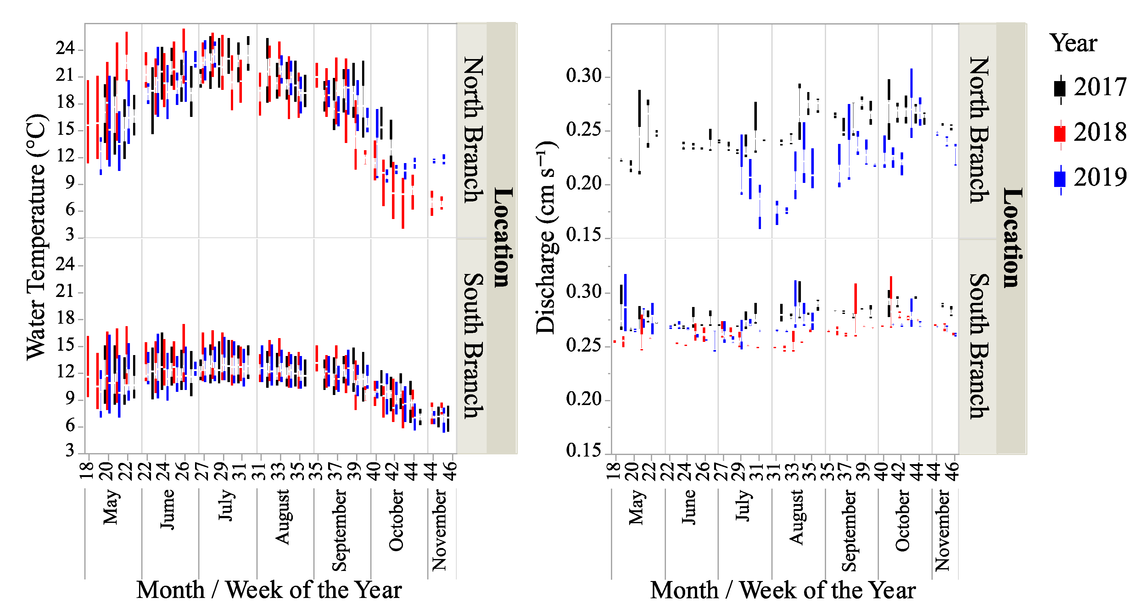
Water temperature and dissolved oxygen were measured every 10 min from mid-May through early November in 2017, 2018, and 2019 using a HOBO® Model U26-001 (Onset Computer Corporation, Bourne, MA, USA) probe. The probes were placed mid-stream in riffle areas and approximately 15 cm above the bottom. Conductivity was measured with a HOBO® Model U24-001 (Onset Computer Corporation, Bourne, MA, USA) probe for 2017 in the North Branch and 2017 and 2018 in the South Branch. Water depth was measured with a HOBO® Model U20L-04 (Onset Computer Corporation, Bourne, MA, USA) probe. A HOBO® weather station was deployed next to the North Branch site in full sunlight. The weather station was outfitted with photosynthetically active radiation (PAR) (HOBO® Model S-LIA-M003, Onset Computer Corporation, Bourne, MA, USA) and barometric pressure sensors (HOBO® Model BPB-CM50, Onset Computer Corporation, Bourne, MA, USA). For a portion of 2018, the PAR sensor malfunctioned. Fortunately, a PAR sensor (Li-Corr® LI-190R sensor, Onset Computer Corporation, Bourne, MA, USA) was functioning at another site 21.8 km away throughout this study. We developed a regression relationship between this more distant site and the Valley Creek site when both were functioning (R2 = 0.86) and an estimate of PAR at Valley Creek was made for the time when the PAR sensor was malfunctioning by taking data from the more distant site. An additional HOBO® PAR sensor was placed in a forested area 250 m upstream of the North Branch sampling site and 600 m from the South Branch site. This allowed for the assessment of the potential impact of forest shading on light availability.
Discharge measures were provided by the Washington County Minnesota Conservation District (Oakdale, MN). On the North Branch, the discharge station was about 250 m upstream of the sampling location. On the South Branch, the station was about 5 m upstream of the sampling location. Discharge data were not available for the North Branch for 2018 and 2019 until 18 July 2019, due to a malfunction of the gauge. Both of the streams are in a well-defined channel with the North Branch being approximately 2.5 m wide during base flow and the South Branch being about 4 m wide at base flow. The South Branch has coarser substrate (average ϕ size = −1.14—fine gravel) than the North Branch (average ϕ size = −0.43—coarse sand) [46]. There are few macrophytes in the channels and with the little biofilm being found on the relatively fine substrates.
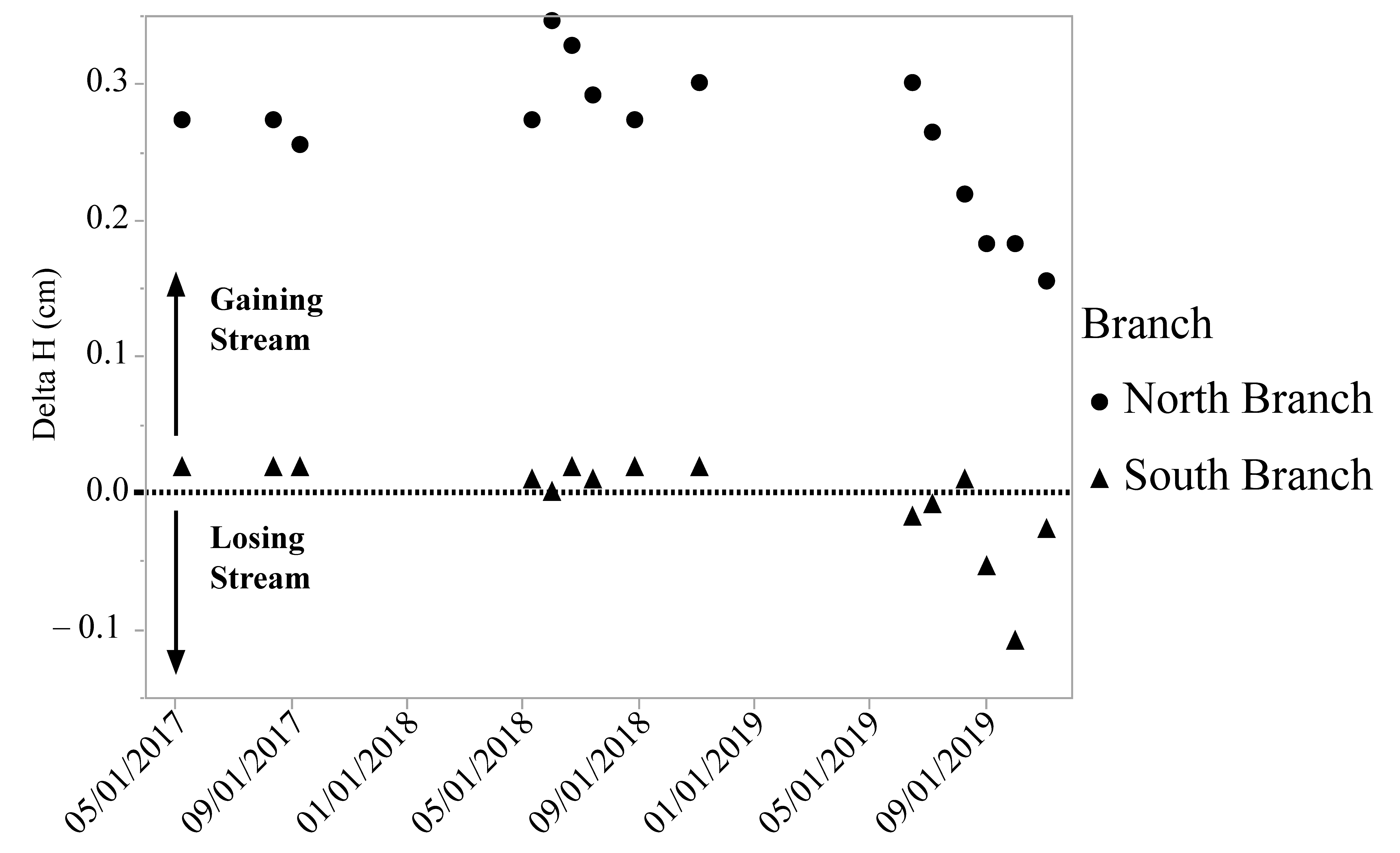
Minipiezometers were installed in both streams to assess the level of groundwater input or recharge (inside diameter—0.7 cm, screen length—4.3 cm) to a depth of 1.1 m below the sediment–water interface. Stream depth and water depth in the piezometer were measured to calculate the vertical hydraulic gradient, an indication of the amount of groundwater entering or leaving a stream [52].
Weather data, including daily precipitation, and maximum and minimum air temperatures were retrieved from the Utah Climate Center (http://climate.usu.edu, accessed on 30 April 2020) for the GHCN:COOP station USC00218039, Stillwater2SW, MN which is approximately 15 km from the study site. Nitrogen (N) and phosphorus (P) levels were measured by the Washington County Conservation District and the St. Croix Watershed Station (Science Museum of Minnesota, Marine on St. Croix, MN, USA) twice each year in 2017–2019.
Differences in the physical and chemical characteristics in the two branches of Valley Creek and between years were assessed using mixed-model ANOVAs. ANOVAs are used to test whether there are significant difference in the means of dependent variables for different values of independent variables. Water temperature, depth, discharge, or conductivity were used as dependent variables and location, year (as nominal variables), and their interactions were used as the independent variables. The day of the year was used as the random variable in these analyses. Since there were few measures of dissolved N and P, two-way ANOVAs were used with location, year, and their interaction as the independent variables. For weather data, only the difference between years was examined. For those factors that were statistically significant at the 5% level, pairwise Tukey tests were used to detect where the differences lie. Tukey tests allow for the comparison of the means of multiple levels of an independent variable after a significant ANOVA test.
2.3. Ecosystem Metabolism
Elements of ecosystem metabolism were determined using the single station method [53], which relies on measuring the daily changes in dissolved oxygen levels. Gross primary production (GPP) was assessed as the increase in oxygen in the stream due to photosynthesis. Ecosystem respiration (ER) was assessed as the decrease in oxygen in the stream due to respiration and assumes that respiration is constant during the day and night. Both GPP and ER were corrected for oxygen loss or gain from the atmosphere, termed reaeration. Finally, net ecosystem production (NEP) was calculated as the amount of production that exceeds GPP. The relationship between these measures of ecosystem metabolism is described in Equations (1) and (2):
where C = concentration of oxygen, Cs = concentration of oxygen at saturation, k = reaeration coefficient, and GWA = oxygen accrual from groundwater. The Bayesian single-station estimation model (BASE—version 2.3) was used to estimate k, GPP, and ER [54]. This model is available as an R-package (https://github.com/dgiling/BASEmetab, accessed on 19 July 2018). To ensure valid estimates of ecosystem metabolism, the convergence of the Markov chain Monte Carlo method used in the model, the posterior prediction fit, the R2 for the model, the effective number of parameters, and the visual fit of the model were all assessed. In 2019, oxygen data were not available from August 3 to August 12 due to issues with the probe, so values of ecosystem metabolism could not be modeled for those dates. Mixed-model ANOVAs were used to test whether there were significant differences between locations and years (as independent nominal variables) for GPP, ER, and NEP, with day of the year as the random variable. The metabolism data were not normally distributed and, thus, were natural log (ln)-transformed. For analysis of ln(NEP), since NEP is often negative, constant (43—the minimum NEP measured) was added to each value to ensure that all values were positive.
NEP = GPP − ER
ANCOVAs were performed to examine the influence of water temperature, light input (PAR), or discharge (covariables) and location (independent variable) and their interaction on ln-transformed ecosystem metabolism parameters dependent variables (GPP, ER, and NEP). ANCOVAs are a blend of ANOVA and linear regression. They test for the difference in the mean of a dependent variable for various levels of an independent variable, while controlling for the effects of a continuous variable (the covariable). For discharge, separate analyses were conducted for the North and South Branches, since discharge data were available for all three years for the South Branch but only for 2017 a July 13–November 8 in 2019 when data were available.
All statistical analyses were conducted with JMP® Pro version 14.2 (SAS Institute, Cary, NC, USA).
3. Results
3.1. Physical–Chemical Parameters
Water temperature was significantly different between locations and years (Table 1 and Table 2, Figure 2) with the water temperature greater in the North Branch than the South Branch. Overall, the water temperature was more variable in the North Branch than the South Branch (coefficient of variation was 17.4 and 27.8% for the South and North Branches, respectively.) Water depth was also significantly different between locations and years with both locations having the greatest depth in 2019 and the lowest depth in 2018 (Table 1 and Table 2). Overall, the water depth was more variable in the North Branch than the South Branch (coefficient of variation 16.8 and 31.9% for the South and North Branches, respectively). Discharge data were only available from the North Branch for 2017 and half of 2019 (Figure 2). Based on comparing these data with those from the South Branch for the same time periods showed that discharge was slightly (but significantly) higher in the South Branch than the North Branch and was higher in 2017 than 2019 for both branches (Table 1 and Table 2).
Discharge was more variable in the North Branch than the South Branch (coefficient of variation 11.8 versus 3.9%, respectively). The conductivity, measured in both locations in 2017 was higher in the North Branch than the South Branch (Table 1, t-test − t39222 = 51.9, p < 0.0001). From data provided by the St. Croix Watershed Research Station (Science Museum of Minnesota—Table 1), there was no significant difference in dissolved P levels between the branches or years (two-way ANOVA—location: F1,11 = 6.8, p = 0.6; year: F2,11 = 1.3, p = 0.3; location*year: F2,11 = 0.7, p = 0.5). There was a significant difference in dissolved N between branches with the South Branch having higher levels of N but no difference between years (two-way ANOVA—location: F1,11 = 249.9, p < 0.0001; year: F2,11 = 1.2, p = 0.4; location*year: F2,11 = 1.0, p = 0.4).
There were no significant differences between years in the amount of light reaching the streams (mixed-model ANOVA—F2,327 = 0.6, p = 0.5). However, for PAR levels measured in the forested part of the stream, there were significant differences (mixed-model ANOVA—F2,288 = 3.1, p = 0.04) with PAR being significantly lower in 2018 than in 2017 or 2019 (Figure 3). There was a large change in PAR values in the forested site over the seasons, with light levels decreasing greatly in early spring (May) and then remaining fairly constant after leaf-out (Figure 3). There was not as much change in PAR in the spring at the open site, used in calculating stream metabolism parameters, but a decline in the fall as the sun angle decreased.
The North Branch is a gaining stream in the section of the creek where the DO levels were measured, while the water in the South Branch is close to being in equilibrium with the groundwater (Figure 4) at the sampling location. For both branches, the exchange between surface and groundwater was fairly stable in 2017 and 2018 with a drop in the gradient in both streams in 2019 (Figure 4).
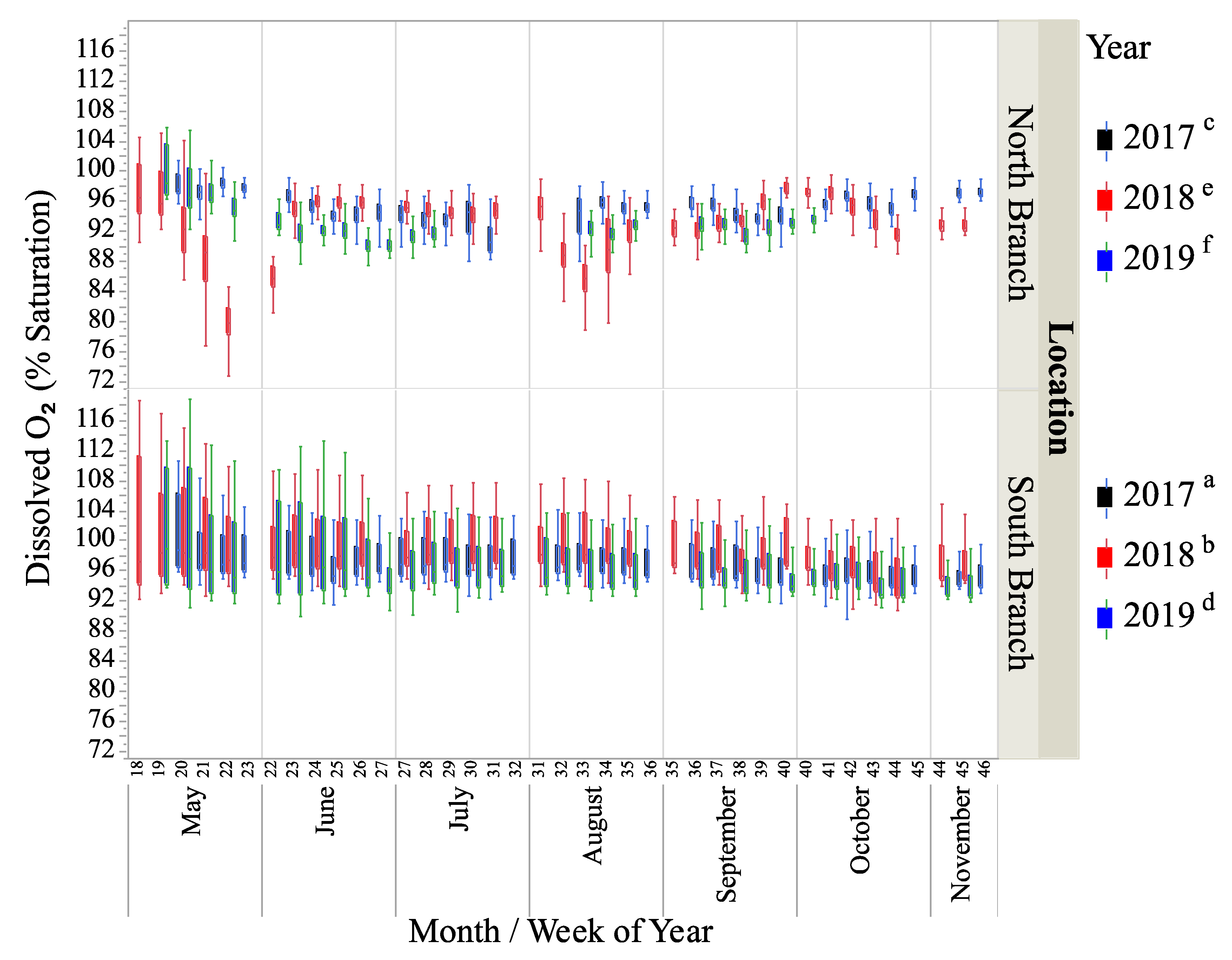
The percent saturation of dissolved oxygen (DO) was significantly different between locations and years (Figure 5, Table 1 and Table 2). Based on a Tukey test of the significant interaction term (Table 2), % DO saturation was greatest in the South Branch in 2018 and 2017, followed by the North Branch in 2017, the South Branch in 2019, and the North Branch in 2018 and 2019, respectively (Figure 5, Table 2). Despite the statistical significance between years and locations, the range of average DO levels was only 93–96.8%. The South Branch on average had a DO saturation of 97.5%, while the North Branch average was 93.8%.
Analysis of weather data indicated that the average daily precipitation varied between years (mixed-model ANOVA—F2,582 = 4.3, p = 0.01) with 2019 being significantly wetter (4.3 mm day−1) than either 2017 or 2018 (2.4 mm day−1 each). The average daily maximum temperature was lower for 2019 than for 2017 or 2018 (mixed-model ANOVA—F2,600 = 8.2, p = 0.0003; 10.1, 11.9, and 11.1 °C for 2019, 2017, and 2018, respectively). There was no significant difference in the minimum daily temperatures between 2017, 2018, or 2019 (mixed-model ANOVA—F2,588 = 2.6, p = 0.07), although 2019 minimum temperatures were lower than 2017 or 2018 (0.6, 1.3, and 1.3 °C for 2019, 2017, and 2018, respectively).
3.2. Ecosystem Metabolism
Rates of ecosystem metabolism were calculated for 1068 days. Of these, 73 days (7%) were excluded from the analysis because the model did not converge or the R2 values for the model fit were less than 0.5. Of these, 21, 23, and 29 days were excluded for 2017, 2018, and 2019, respectively, and 70 of the 73 were for the North Branch location.
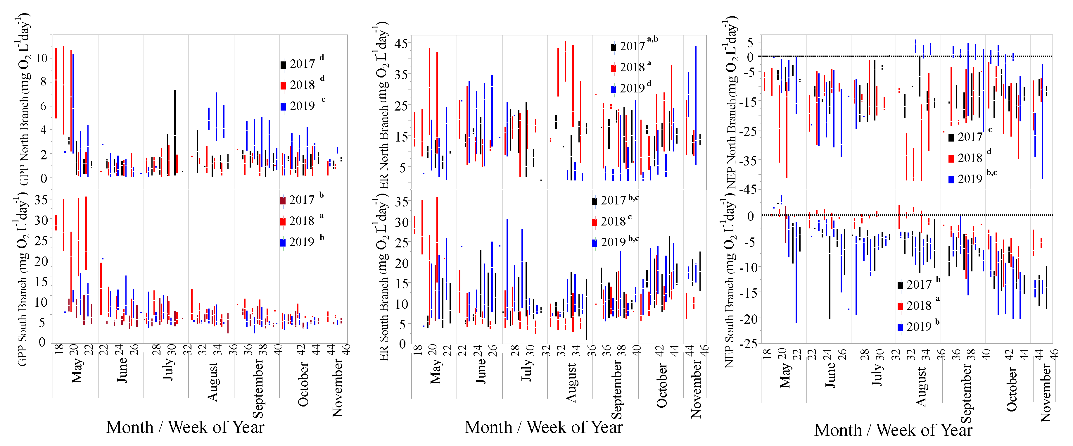
There were significant differences for GPP, ER, and NEP between years and locations and their interaction (Figure 6, Table 2). A Tukey test indicated that GPP was significantly lower in 2017 than in 2018 or 2019 (Table 3). GPP was greater in the South Branch than the North Branch (Table 3). The significant interaction term (Table 2) showed that GPP was highest in 2019 in the North Branch, but highest in 2018 for the South Branch (Table 3). GPP was also highest in May in most years (Figure 6).
For ER, there were significant differences between years but not between locations (Figure 6, Table 2). However, there was a significant interaction between location and year; thus, location did play a role in the differences between years. For ER, there was no significant difference between years for the South Branch, while for the North Branch, ER was significantly lower in 2019 than in 2017 or 2018 (Table 3). Generally, ER was lower in the South Branch than the North Branch except for 2019 (Table 3).
NEP was generally < 0 for both locations and all 3 years (Figure 6). There were significant differences between locations and years in NEP (Figure 6, Table 2). NEP was generally greater (less negative) in the South Branch than the North Branch except for 2019 (Table 3). NEP was greatest in the South Branch in 2018, while it was lowest in 2018 for the North Branch, demonstrating the importance of the interaction term (Table 2 and Table 3).
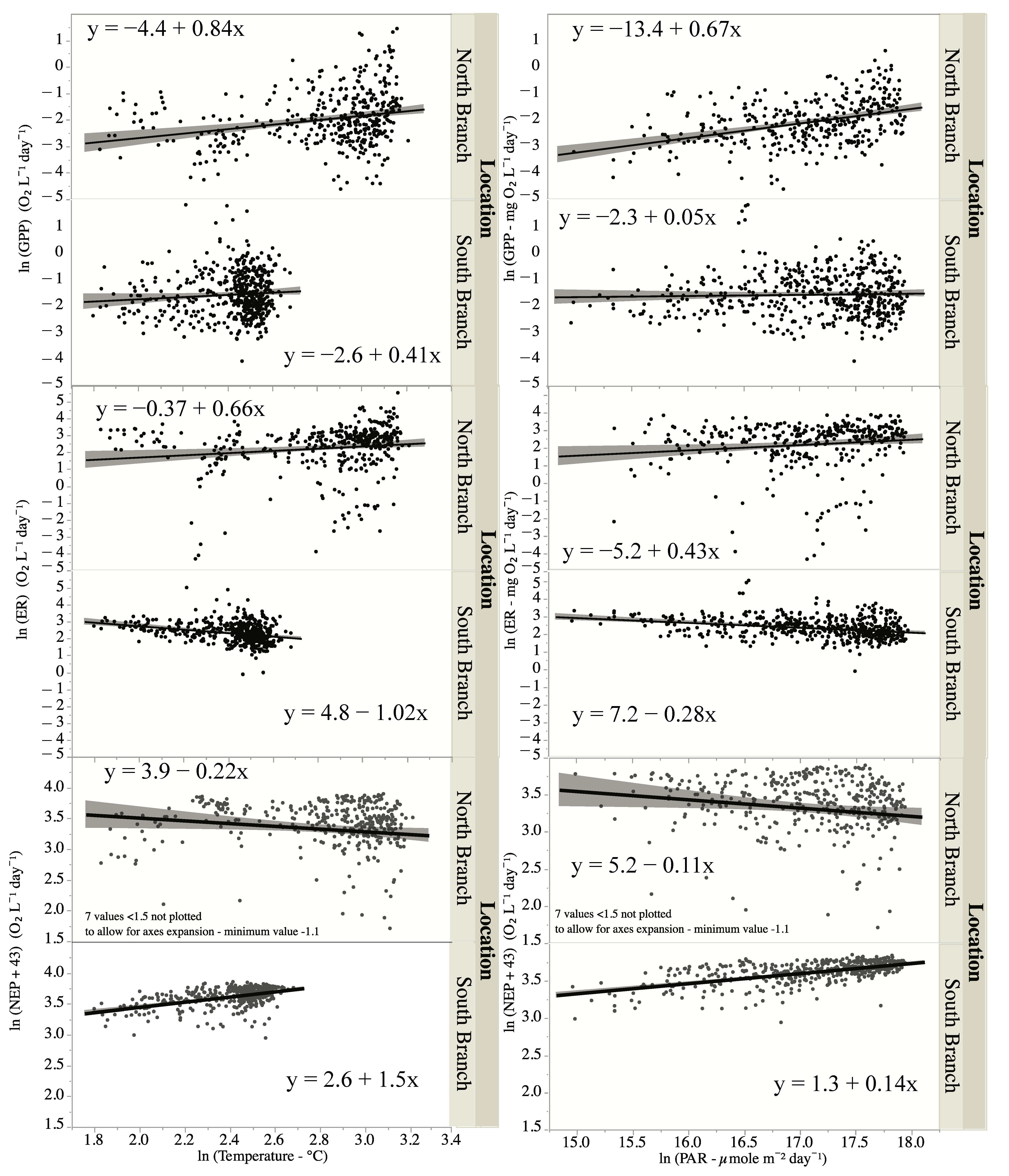
An ANCOVA showed that water temperature had a significant impact on GPP and through significant interaction terms on ER and NEP (Table 4). Since there was no significant interaction term for GPP, thus, the temperature impacts on GPP were similar although small (Figure 7). There was an increase in ER with temperature in the North Branch but a small but negative effect in the South Branch (Figure 7). For NEP, the increased temperature had a positive effect on NEP in the South Branch but a negative effect in the North Branch (Figure 7).
Light intensity, measured as PAR, had a significant impact on GPP, and this impact varied by location (Figure 7, Table 5). The impact was greater for the North Branch than the South Branch (Figure 7). PAR did not have a significant effect on either ER or NEP except through its interaction with location (Figure 7, Table 5). For the North Branch, there was a slight positive effect of PAR on ER but a slight negative effect in the South Branch. For NEP, the effects of PAR were just the opposite; slightly negative for the South Branch and slightly negative for the North Branch (Figure 7). PAR used in these calculations were from a sensor in full sunlight.
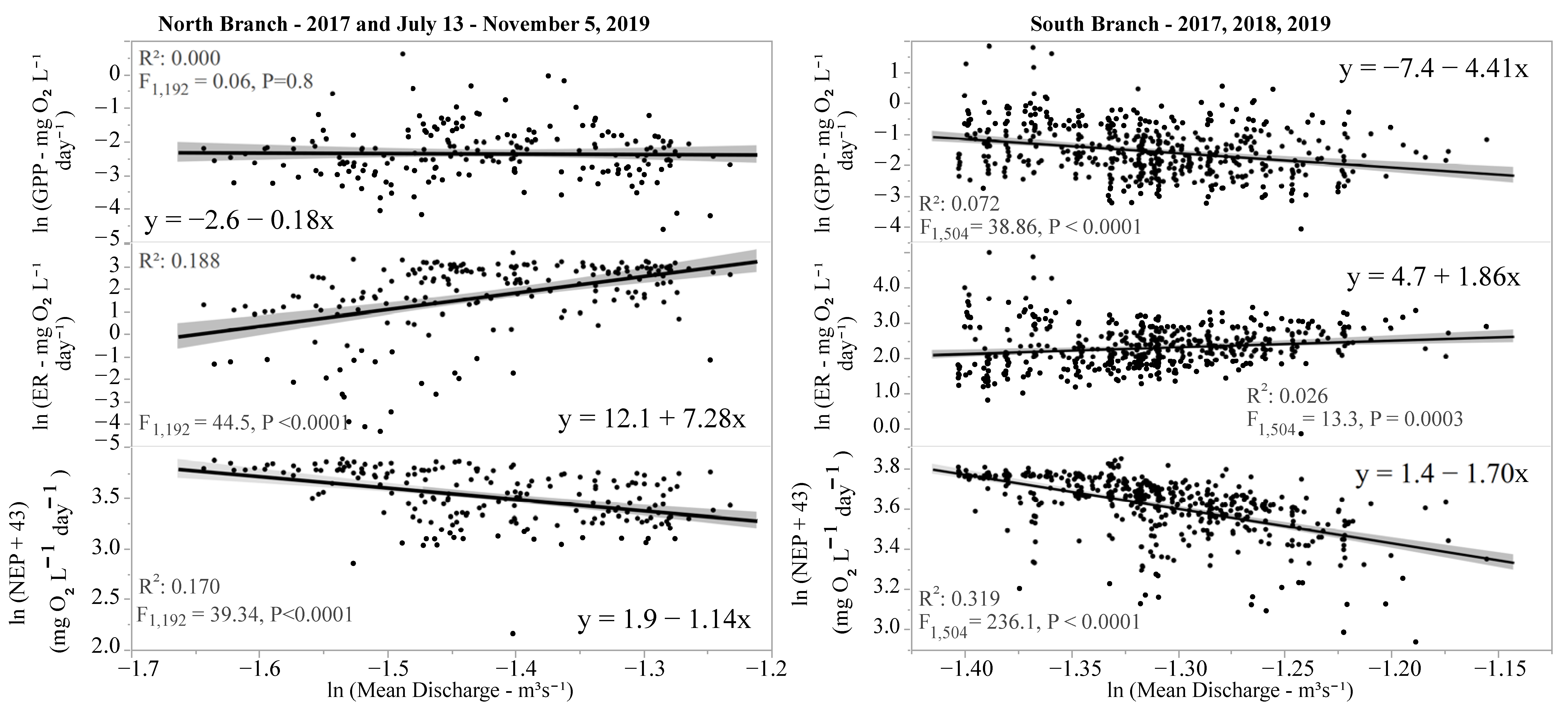
Since there were no discharge data for the North Branch for 2018 and May–early July 2019, the relationship between discharge and ecosystem metabolism was examined separately for each location. There was a small but negative impact of discharge on GPP in the South Branch but no impact in the North Branch (Figure 8). In both locations, discharge was positively correlated with ER, resulting in significant negative relationships between discharge and NEP (Figure 8). The R2 values were quite low for these regressions, indicating that while in most cases there was a significant influence of discharge on various components of stream metabolism, the effect was quite modest, at most explaining 32% of the variability in NEP and often explaining less than 20% (Figure 8).
4. Discussion
This study found differences in measures of ecosystem metabolism between the two branches of Valley Creek with differences between years. There were also significant impacts of temperature, PAR, and discharge for at least some measures of stream metabolism. Several factors can influence aquatic ecosystem metabolism. These include temperature, light intensity, hydrologic disturbance [42,55,56], fish spawning [57], nutrient input [58,59], and urban local inflows [60]. Land use and riparian canopy cover influence GPP, with agricultural, grassland, and urban streams having higher GPP than forested or desert streams, but little difference in ER between land-use types [61].
Changes in dissolved oxygen levels are used to calculate ecosystem metabolism [60]. Both biotic and abiotic factors can influence the oxygen content in stream systems. Biotic influences include primary production and respiration [62], which are reflected in measures of ecosystem metabolism. Abiotic factors include temperature, water velocity, and oxygen exchange with the atmosphere and groundwater [62,63]. There were differences in oxygen levels between the two locations in this study and between years. Hornbach et al. [46] found that the dissolved oxygen level in groundwater was lower than surface water in both of the locations in this study (10.8 versus 93% saturation in groundwater and surface water in the North Branch, respectively, and 23 vs. 95% saturation in groundwater and surface water in the South Branch, respectively). Groundwater input can have a substantial impact on the measurement of steam metabolism [64], although more research is needed into the role of groundwater input on these measures [65]. Some of the differences in the dissolved oxygen levels and measures of ecosystem metabolism between branches could be explained by the North Branch’s greater groundwater input and its lower DO content. In 2019, the groundwater hydraulic head was lower in both streams, indicating less groundwater input into the streams. However, the DO levels in 2019 were not significantly higher than in either 2017 or 2018. In 2019, the weather was wetter and cooler than the other years in this study. This may have resulted in the greater stream water depth found, and if the groundwater level stayed the same then, the hydraulic head would be lower. Despite the greater water depth in 2019, it did not result in greater discharge. This could be a result of water depth being measured for the full sampling period, but discharge data are only available for July–November 5. Consequently, the impact of the differing groundwater inputs on DO between years is difficult to ascertain.
Hornbach et al. [46] found that the groundwater in both branches had low levels of oxygen (10.8 and 23.0% for the North and South Branches, respectively). This resulted in the North Branch site having a mean bias in GPP (GPP uncorrected for groundwater/GPP corrected for groundwater) of 0.57, indicating GPP estimates may be lower than if corrected for groundwater input. For ER, the bias was 1.12, indicating that our measures of ER may be higher than if corrected for groundwater input. Both GPP and ER were only measured in the fall in the 2015 study. However, the groundwater input in the North Branch were fairly steady throughout the 2017–2019 period with a slight decrease in 2019. Applying the 0.57 bias for GPP brings the levels of GPP up, but all were still lower than the level of GPP in the South Branch. For ER, applying the 1.17 bias does not affect the ranking of ER between years and locations. There may be unaccounted for changes in DO concentrations in the aquifer, which, in addition to changes in groundwater input, could influence changes in the measures of DO in this study. Water table level, flooding, and rainfall inputs can all influence subsurface DO levels resulting in seasonal and diel changes in groundwater DO levels ranging from hypoxic to 91% saturation [66].
Even when GPP levels in the North Branch were corrected for groundwater input, the South Branch had higher GPP levels, which was unexpected given the colder temperature of this stream. Hornbach et al. [46] found similar results for the fall of 2015 with GPP higher in the South Branch. They also found that periphyton production was higher in the North Branch than the South Branch, which was also unexpected given the higher GPP in the South Branch. They found that nutrient additions, especially of P, increased periphyton production in both streams, suggesting it may be a limiting nutrient. The levels of N in both branches are considered relatively high (>1 mg/L), while phosphorus levels are considered low (<0.1 mg/L) [67]. Nitrogen levels were higher in the South Branch, which might support greater GPP. The lower N levels in the North Branch may be due to denitrification occurring in the wetlands associated with Lake Edith at the head of this branch. While nutrient levels may not be greatly important in influencing GPP, nitrate-N was the third most important predictor of GPP after temperature and light [68]. However, even though nutrient levels within a river are often poorly correlated with GPP, nutrient supplies, rather than concentrations, often limit GPP [68]. The land use in the South Branch contains more cultivated crops and hay/pasture land than the North Branch [69], and thus, nutrient supplies may be greater in the South Branch supporting higher GPP. Another possibility is that there are differences in the types of primary producers in the two branches. Autotrophs from cold-water streams can have higher photosynthetic rates than those from warmer streams and which could lead to higher GPP in cold-water streams [70].
Several studies have shown that there are both seasonal and interannual variation in ecosystem metabolism. There are two major types of seasonal variability in U.S. rivers: a summer peak or a spring peak [71]. Spring peak rivers had daily patterns of GPP that were only weakly correlated with water temperature, discharge, or PAR and tend to be associated with smaller watersheds such as headwater streams. In this study, GPP was higher in the spring and corresponded to a time when light levels were greater in the forested area near the sampling sites. Seasonal patterns of ecosystem metabolism can be greatly affected by leaf phenology, with higher rates of GPP rates and NEP approaching autotrophy under an open canopy in the spring [44,56]. Models with season as a main effect were the best predictors of GPP, ER, and NEP [72], with approximately 50% of the variation in GPP and ER related to season [43]. The sag in percent oxygen in the North Branch in May and August of 2018 could be due to inputs of organic material from the surrounding wetland. This corresponded to peaks of ER during these months.
In addition to seasonal variability, there can be interannual variability in ecosystem metabolism in streams attributable to a combination of light availability, water temperature, storm flow, and desiccation [44,73]. In this study, interannual variation differed between the two locations. GPP was higher in the South Branch than the North Branch in each year of the study, even though water temperatures were colder and P levels were similar. However, the years in which GPP peaked differed between branches. In the North Branch, GPP was the highest in 2019, but in the South Branch, it was the highest in 2018. Interannual variation was different for ER, being the highest for the North Branch in 2018, with no significant difference between years for the South Branch. The North Branch was more heterotrophic than the South Branch with NEP greatest for the South Branch in 2018 and in 2019 for the North Branch with higher levels of GPP driving these trends.
Since seasonal and interannual variability in ecosystem metabolism could be due to differences in temperature, PAR, and discharge, we examined the correlations between these factors and GPP, ER, and NEP. As expected [65,74,75], PAR was positively correlated with GPP in both locations. The slope for PAR versus GPP was greater in the North Branch than in the South Branch (0.6 versus 0.04 for the North and South branches, respectively) indicating a great impact of PAR on GPP in the North Branch. Hornbach et al. [46] found that instream light levels were greater in the North Branch than the South Branch and that periphyton production, at least in the fall, was greater in the North Branch. This could account for the greater impact of light on GPP. Water temperature and PAR can interact synergistically with higher water temperature, enhancing the response of PAR on GPP [73], which was apparently the case in the warmer North Branch. However, the correlation between PAR and temperature makes disentangling the impacts of temperature and PAR difficult [76].
While there were significant interaction terms between PAR and location with both ER and NEP, there were no significant main effects (PAR only), indicating that most of the difference in the interaction term stemmed from the differences between the branches. Since ER in streams may be more influenced by allochthonous sources of carbon than autochthonous sources [75,77], the lack of relationship between PAR and ER was not unexpected. NEP is correlated with PAR, but mainly through its influence on GPP and not ER [76].
Water temperature was positively correlated with GPP in both locations. ER on the other hand was positively correlated with temperature in the North Branch but negatively correlated in the South Branch. The slope for temperature versus GPP was 0.8 for the North Branch and 0.7 for ER, indicating that the impact of temperature was similar for both GPP and ER at this site. For the South Branch, the slope of the temperature versus GPP was 0.4, while the slope was −1.0 for temperature versus ER, indicating differential impacts of temperature on GPP and ER. Unlike this study where there was either little difference in temperature effects between GPP and ER (North Branch) or where temperature had different impacts on GPP than ER (South Branch), others have found that temperature had a greater influence on ER than on GPP [78]. This was attributed to the higher temperature dependence of respiration compared to photosynthesis [78]. Others, however, have found that temperature sensitivities of GPP and ER at the ecosystem level may not follow the differential sensitivities to temperature at the cellular level [41], while still, others have found that GPP did not vary with temperature when adjusted for differences in autotrophic biomass [70]. The temperature dependence of ER could be influenced by the amount of dissolved organic matter (DOM) with ER increasing more with temperature with higher amounts of DOM [79]. Since the North Branch was found in a wetland, it may have received more DOM than the South Branch resulting in the greater dependence of ER on temperature in this branch.
The negative relationship between temperature and ER was unexpected in the South Branch, but there was little variation in temperature in this branch (~13 °C). The R2 for this relationship was only 0.09, indicating little impact of temperature on ER. The greater effect of temperature on both ER and GPP in the North Branch could be due to the greater temperature range experienced there (~23 °C). Generally, NEP increases with temperature due to the greater temperature sensitivity of ER relative to GPP [41,78]. In this study, NEP increased with increasing temperature in the South Branch but not in the North Branch. In the South Branch, the negative relationship between ER and temperature drove NEP to be positively correlated with temperature (GPP increased while ER decreased), while in the North Branch, the similar impact of temperature on GPP and ER results in no change in NEP with temperature.
Discharge had no effect on GPP in the North Branch and a small but negative impact in the South Branch. While some have found little correlation between discharge and GPP [45], others found that in large rivers increased discharge may have a negative relationship with GPP presumably due to light attenuation in these systems [75]. A positive correlation between discharge and ER, similar to that found in this study, has been noted [45,75], likely due to the greater amounts of allochthonous material reaching streams and rivers resulting in higher ER. The impact of discharge on ER was greater in the North Branch than the South Branch (slope 7.3 versus 1.9 for the North and South Branches, respectively). The North Branch sampling location is in a wetland area, and greater discharge may bring in larger amounts of allochthonous materials or dissolved organic carbon (DOC) than in the South Branch resulting in increased ER [80]. In both branches, NEP decreased, likely due to the increased ER.
5. Conclusions
It was predicted that gross primary production and ecosystem respiration would be greater when temperatures were warmer both seasonally and between years and that the streams might be autotrophic in the spring when light availability is greatest (less shading from the surrounding forest). It was also expected that higher discharge might influence ecosystem respiration bringing in more allochthonous material to be decomposed. Within our streams, increasing temperature was correlated with increased GPP, as predicted. However, between streams, the colder stream had higher levels of GPP each year, which could be due to differences in N availability and/or differences in autotrophic communities. There was increased GPP in the spring apparently correlated with greater light intensity before leaf-out and increased ER with increase discharge. The years of peak GPP and ER differed between sites indicating the need for long-term monitoring at multiple locations.
While the continuous monitoring of various parameters (temperature, conductivity, discharge, and PAR) assisted with the examination of those factors influencing ecosystem metabolism in this study, monitoring of other features that might be important in explaining both annual and interannual variability would be helpful. Continuous monitoring of chl a, soluble reactive phosphorus, turbidity, and others, important in influencing ecosystem metabolism, is needed to enhance our understanding of the response of aquatic ecosystems to changing human impacts and climate [81].
Funding
This research received no external funding.
Data Availability Statement
The data presented in this study are available on request from the corresponding author.
Acknowledgments
I would like to acknowledge the Belwin Conservancy for providing access to Valley Creek. Thanks to Ken Moffett who constructed the piezometers and holders for the water sensors and to Jim Almendinger of the St. Croix Watershed Research Station of the Science Museum of Minnesota for providing water quality data. Erik Anderson from the Washington County Watershed District, MN provided discharge data. Thanks to the Macalester College Aquatic Ecology class who helped collect data in the fall of 2017. Additionally, thanks to Mark Hove who helped install water sensors and retrieve data on many occasions.
Conflicts of Interest
The author declares no conflict of interest. The funders had no role in the design of the study; in the collection, analyses, or interpretation of data; in the writing of the manuscript, or in the decision to publish the results.
References
- Caissie, D. The thermal regime of rivers: A review. Freshw. Biol. 2006, 51, 1389–1406. [Google Scholar] [CrossRef]
- Heino, J.; Virkkala, R.; Toivonen, H. Climate change and freshwater biodiversity: Detected patterns, future trends, and adaptations in northern regions. Biol. Rev. 2009, 84, 39–54. [Google Scholar] [CrossRef] [PubMed]
- Markovic, D.; Carrizo, S.F.; Kärcher, O.; Walz, A.; David, J.N.W. Vulnerability of European freshwater catchments to climate change. Glob. Change Biol. 2017, 23, 3567–3580. [Google Scholar] [CrossRef]
- Pyne, M.I.; Poff, L. Vulnerability of stream community composition and function to projected thermal warming and hydrologic change across ecoregions in the western United States. Glob. Change Biol. 2017, 23, 77–93. [Google Scholar] [CrossRef] [PubMed] [Green Version]
- Bernhardt, E.S.; Heffernan, J.B.; Grimm, N.B.; Stanley, E.H.; Harvey, J.W.; Arroita, M.; Appling, A.P.; Cohen, M.J.; McDowell, W.H.; Hall, R.O., Jr.; et al. The metabolic regimes of flowing waters. Limnol. Oceanogr. 2018, 63, S99–S118. [Google Scholar] [CrossRef] [Green Version]
- Coffey, R.; Paul, M.J.; Stamp, J.; Hamilton, A.; Johnson, T. A review of water quality responses to air temperature and precipitation changes 2: Nutrients, algal blooms, sediment, pathogens. J. Am. Water Resour. Assoc. 2019, 55, 844–868. [Google Scholar] [CrossRef]
- Paul, M.J.; Coffey, R.; Stamp, J.; Johnson, T. A review of water quality responses to air temperature and precipitation changes 1: Flow, water temperature, saltwater intrusion. J. Am. Water Resour. Assoc. 2019, 55, 824–843. [Google Scholar] [CrossRef]
- O’Briain, R. Climate change and European rivers: An eco-hydromorphological perspective. Ecohydrology 2019, 12. [Google Scholar] [CrossRef]
- Knouft, J.H.; Ficklin, D.L. The potential impacts of climate change on biodiversity in flowing water systems. Ann. Rev. Ecol. Syst. 2017, 48, 111–133. [Google Scholar] [CrossRef]
- Niedrist, G.H.; Füreder, L. Real-time warming of alpine streams: (re)defining invertebrates’ temperature preferences. River Res. Applic. 2020, 1–11. [Google Scholar] [CrossRef]
- Bogardi, J.J.; Leentvaar, J.; Sebesvárl, Z. Biologia Futura: Integrating freshwater ecosystem health in water resources management. Biol. Futur. 2020, 71, 337–358. [Google Scholar] [CrossRef]
- O’Gorman, E.J.; Pichler, D.E.; Adams, G.; Benstead, J.P.; Cohen, H.; Craig, N.; Cross, W.F.; Demars, B.O.L.; Friberg, N.; Gislason, G.M.; et al. Impacts of warming on the structure and functioning of aquatic communities: Individual-to-ecosystem-level responses. Adv. Ecol. Res. 2012, 47, 81–176. [Google Scholar] [CrossRef] [Green Version]
- Fullerton, A.H.; Torgersen, C.E.; Lawler, J.J.; Steel, E.A.; Ebersole, J.L.; Lee, S.Y. Longitudinal thermal heterogeneity in rivers and refugia for coldwater species: Effect of scale and climate change. Aquat. Sci. 2018, 80, 1–15. [Google Scholar] [CrossRef] [PubMed]
- Fenoglio, S.; Bo, T.; Cucco, M.; Mercalli, L.; Malacarne, G. Effects of global climate change on freshwater biota: A review with special emphasis on the Italian situation. Ital. J. Zool. 2010, 77, 374–383. [Google Scholar] [CrossRef]
- Haase, P.; Pilotto, F.; Li, F.; Sunderman, A.; Lorenz, A.W.; Tonkin, J.D.; Stoll, S. Moderate warming over the past 25 years has already reorganized stream invertebrate communities. Sci. Total Environ. 2019, 658, 1531–1538. [Google Scholar] [CrossRef]
- Isaak, D.J.; Wollrab, S.; Horan, D.; Chandler, G. Climate change effects on stream and river temperatures across the northwest U.S. from 1980–2009 and implications for salmonid fishes. Climactic Chang. 2012, 113, 499–524. [Google Scholar] [CrossRef] [Green Version]
- Selbig, W.R. Simulating the effect of climate change on stream temperature in the Trout Lake Watershed, Wisconsin. Sci. Total Environ. 2015, 521, 11–18. [Google Scholar] [CrossRef]
- Lynch, A.J.; Myers, B.J.E.; Chu, C.X.; Eby, L.A.; Falke, J.A.; Kovach, R.P.; Krabbenhoft, T.J.; Kwak, T.J.; Lyons, J.; Paukert, B.P.; et al. Climate change effects on North American inland fish populations and assemblages. Fisheries 2016, 41, 346–361. [Google Scholar] [CrossRef]
- Biswas, S.R.; Vogt, R.J.; Sharma, S. Projected compositional shifts and loss of ecosystem services in freshwater fish communities under climate change scenarios. Hydrobiologia 2017, 799, 135–149. [Google Scholar] [CrossRef]
- Mitro, M.G.; Lyons, J.D.; Stewart, J.S.; Cunningham, P.K.; Griffin, J.D.T. Projected changes in brook trout and brown trout distribution in Wisconsin streams in the mid-twenty-first century in response to climate change. Hydrobiologia 2019, 840, 215–226. [Google Scholar] [CrossRef]
- Johnson, Z.C.; Snyder, C.D.; Hitt, N.P. Landform and season precipitation predict shallow groundwater influence on temperature in headwater streams. Water Resour. Res. 2017, 53, 5788–5812. [Google Scholar] [CrossRef]
- Leach, J.A.; Moore, R.D. Empirical stream thermal sensitivities may underestimate stream temperature response to climate warming. Water Resour. Res. 2019, 55, 5453–5467. [Google Scholar] [CrossRef]
- Carlson, A.K.; Taylor, W.W.; Infante, D.M. Modelling effects of climate change on Michigan brown trout and rainbow trout: Precipitation and groundwater as key predictors. Ecol. Freshw. Fish 2020, 29, 433–449. [Google Scholar] [CrossRef]
- Tank, J.L.; Rosi-Marshall, E.J.; Griffiths, N.A.; Entrekin, S.A.; Stephen, M.L. A review of allochthonous organic matter dynamics and metabolism in streams. J. N. Am. Benthol. Soc. 2010, 29, 118–146. [Google Scholar] [CrossRef] [Green Version]
- Hall, R.O. Metabolism of streams and rivers: Estimation, controls and application. In Stream Ecosystems in a Changing Environment; Jones, J.B., Stanley, E.H., Eds.; Academic Press: New York, NY, USA, 2016; pp. 151–180. [Google Scholar] [CrossRef]
- Demars, B.O.L.; Thompson, J.; Manson, J.R. Stream metabolism and the open diel oxygen method: Principles, practice, and perspectives. Limnol. Oceanogr. Methods 2015, 13, 356–374. [Google Scholar] [CrossRef] [Green Version]
- Siders, A.C.; Larson, D.M.; Rüegg, J.; Dodds, W.K. Probing whole-stream metabolism: Influence of spatial and heterogeneity on rate estimates. Freshw. Biol. 2017, 62, 711–723. [Google Scholar] [CrossRef]
- Rodríguez-Castillo, T.; Estévez, E.; González-Ferreras, A.M.; Barquín, J. Estimating ecosystem metabolism to entire river networks. Ecosystems 2019, 22, 892–911. [Google Scholar] [CrossRef]
- Young, R.G.; Matthaei, C.D.; Townsend, C.R. Organic matter breakdown and ecosystem metabolism: Functional indicators for assessing river ecosystem health. J. North Am. Benthol. Soc. 2008, 27, 605–625. [Google Scholar] [CrossRef]
- Irwin, C.E.; Culp, J.M.; Yates, A.G. Spatio-temporal variation of benthic metabolism in a large, regulated river. Can. Water Resour. J. 2020, 45, 144–157. [Google Scholar] [CrossRef]
- Staehr, P.A.; Testa, J.M.; Kemp, W.M.; Cole, J.J.; Sand-Jensen, K.; Smith, S.V. The metabolism of aquatic ecosystems: History, applications and future challenges. Aquat. Sci. 2012, 74, 15–29. [Google Scholar] [CrossRef]
- Young, R.G.; Collier, K.J. Contrasting responses to catchment modification among a range of functional and structural indicators of river ecosystem health. Freshw. Biol. 2009, 54, 2155–2170. [Google Scholar] [CrossRef] [Green Version]
- Silva-Junior, E.F. Land use effects and stream metabolic rates: A review of ecosystem response. Acta Limnol. Bras. 2016, 28, e2016103. [Google Scholar] [CrossRef] [Green Version]
- von Schiller, D.; Acuña, V.; Aristi, I.; Arroita, M.; Basaguren, A.; Bellin, A.; Boyero, L.; Butturini, A.; Ginebreda, A.; Kalogianni, E.; et al. River ecosystem processes; a synthesis of approaches, criteria of use and sensitivity to environmental stressors. Sci. Total Environ. 2017, 569–597, 465–480. [Google Scholar] [CrossRef] [PubMed]
- Huang, W.; Liu, X.B.; Peng, W.Q.; Wu, L.X.; Yano, S.; Zhang, J.M.; Zhao, F. Periphyton and ecosystem metabolism as indicators of river ecosystem response to environmental flow restoration in a flow-reduced river. Ecol. Indic. 2018, 92, 394–401. [Google Scholar] [CrossRef]
- Clapcott, J.E.; Young, R.G.; Neale, M.W.; Doehring, K.; Barmuta, L.A. Land use affects temporal variation in stream metabolism. Freshw. Sci. 2016, 35, 1164–1175. [Google Scholar] [CrossRef] [Green Version]
- Pearce, N.J.T.; Yates, A.G. Agricultural best management practice abundance and location does not influence stream ecosystem function or water quality in the summer season. Water 2015, 7, 6861–6876. [Google Scholar] [CrossRef] [Green Version]
- Qasem, K.; Vitousek, S.; O’Connor, B.; Hoellein, T. The effect of floods on ecosystem metabolism in suburban streams. Freshwater Sci. 2019, 38, 412–424. [Google Scholar] [CrossRef]
- Battin, T.J.; Luyssaert, S.; Kaplan, L.A.; Aufdenkampe, A.K.; Richter, A.; Tranvik, L.J. The boundless carbon cycle. Nat. Geosci. 2009, 2, 598–600. [Google Scholar] [CrossRef]
- Hefferman, J.B. Stream metabolism heats up. Nat. Geosci. 2018, 11, 384–385. [Google Scholar] [CrossRef]
- Song, C.; Dodds, W.K.; Rüegg, J.; Argerich, A.; Baker, C.L.; Bowden, W.B.; Douglas, M.M.; Farrell, K.J.; Flinn, M.B.; Garcia, E.A.; et al. Continential-scale decrease in net primary productivity in streams due to climate warming. Nat. Geosci. 2018, 11, 415–420. [Google Scholar] [CrossRef]
- Koenig, L.E.; Helton, A.M.; Savoy, P.; Bertuzzo, E.; Heffernan, J.B.; Hall, R.O., Jr.; Bernhardt, E.S. Emergent productivity regimes of river networks. Limnol. Oceanogr. Lett. 2019, 4, 173–181. [Google Scholar] [CrossRef] [Green Version]
- Uehlinger, U.R.S. Annual cycle and inter-annual variability in gross primary production and ecosystem respiration in a flood prone river during a 15-year period. Freshw. Biol. 2006, 51, 938–950. [Google Scholar] [CrossRef]
- Roberts, B.J.; Mulholland, P.J.; Hill, W.R. Multiple scales of temporal variability in ecosystem metabolism rates: Results from 2 years of continuous monitoring in a forested headwater stream. Ecosystems 2007, 10, 588–606. [Google Scholar] [CrossRef]
- Summers, B.M.; Van Horn, D.J.; González-Pinzón, R.; Bixby, R.J.; Grace, M.R.; Sherson, L.R.; Crossey, L.J.; Stone, M.C.; Parmenter, R.R.; Compton, T.S.; et al. Long-term data reveal highly-variable metabolism and transitions in trophic status in a montane stream. Freshw. Sci. 2020, 39, 241–255. [Google Scholar] [CrossRef]
- Hornbach, D.M.; Hove, M.; Agata, M.; Arnold, E.; Cavazos, E.; Friedman, C.; Jay, K.; Johnson, E.; Johnson, K.; Staudenmaier, A. Ecosystem Structure and Function in two branches of an eastern Minnesota trout stream. J. Freshw. Ecol. 2016, 31, 487–507. [Google Scholar] [CrossRef] [Green Version]
- Fellows, C.D.; Valett, H.M.; Dahm, C.N.; Mulholland, P.J.; Thomas, S. Coupling nutrient uptake and energy flow in headwater streams. Ecosystems 2006, 9, 788–804. [Google Scholar] [CrossRef] [Green Version]
- Mulholland, P.J.; Thomas, S.A.; Valett, H.M.; Webster, J.R.; Beaulieu, J. Effects of light on NO3- uptake in small forested streams: Diurnal and day-to-day variations. J. N. Am. Benthol. Soc. 2006, 25, 583–595. [Google Scholar] [CrossRef]
- Rasmussen, J.J.; Baattrup-Pedersen, A.; Riis, T.; Friberg, N. Stream ecosystem properties and processes along a temperature gradient. Aquat. Ecol. 2011, 45, 231–242. [Google Scholar] [CrossRef] [Green Version]
- Metropolitan Council. Comprehensive Water Quality Assessment of Select Metropolitan Area Streams. St. Paul: Metropolitan Council. 2014. Available online: https://metrocouncil.org/Wastewater-Water/Services/Water-Quality-Management/Stream-Monitoring-Assessment/St-Croix-River-Tributary-Streams-Assessment/St-Croix-Trib-Assessment-Reports/Valley-Creek-Section.aspx (accessed on 22 May 2020).
- Almendinger, J.E. Watershed Hydrology of Valley Creek and Browns Creek: Trout Streams Influenced By Agriculture and Urbanization in Eastern Washington County, Minnesota, 1998_99. 2003. Marine on St. Croix (MN): St. Croix. Watershed Research Station, Science Museum of Minnesota. Available online: https://www.smm.org/sites/default/files/public/attachments/2003_almendinger._watershed.pdf (accessed on 22 May 2020).
- Baxter, C.; Hauer, F.C.; Woessner, W. Measuring groundwater-stream water exchange: New techniques for installing minipiezometers and estimating hydraulic conductivity. Trans Am. Fish Soc. 2003, 132, 493–502. [Google Scholar] [CrossRef]
- Odum, H.T. Primary production in flowing waters. Limnol. Oceanogr. 1956, 1, 102–117. [Google Scholar] [CrossRef]
- Grace, M.; Giling, D.P.; Hladyz, S.; Caron, V.; Thompson, R.M.; Mac Nally, R. Fast processing of diel oxygen curves: Estimating stream metabolism with BASE (BAyesian Single-station Estimation). Limnol. Oceanogr. Methods 2015, 13, 103–114. [Google Scholar] [CrossRef]
- Uehlinger, U. Resistance and resilience of ecosystem metabolism in a flood prone river system. Freshw. Biol. 2000, 4, 319–332. [Google Scholar] [CrossRef]
- Roberts, B.J.; Mulholland, P.J. In-stream biotic control on nutrient biochemistry in a forested stream, West Fork of Walker Branch. J. Geophys. Res. 2007, 112, G04002. [Google Scholar] [CrossRef] [Green Version]
- Benjamin, J.R.; Bellmore, J.R.; Watson, G.A. Response of ecosystem metabolism to low densities of spawning Chinook Salmon. Freshw. Sci. 2016. [Google Scholar] [CrossRef] [Green Version]
- Jabiol, J.; Gossiaux, A.; Lecerf, A.; Rota, T.; Guérold, F.; Danger, M.; Poupin, P.; Gilbert, F.; Chauvet, E. Variable temperature effects between heterotrophic stream processes and organisms. Freshw. Biol. 2020, 65, 1543–1554. [Google Scholar] [CrossRef]
- Pearce, N.J.T.; Thomas, K.E.; Chambers, P.A.; Venkiteswaran, J.J.; Yates, A.G. Metabolic regimes of three mid-order streams in southern Ontario, Canada exposed to contrasting sources of nutrients. Hydrobiologia 2020, 847, 1925–1942. [Google Scholar] [CrossRef]
- Rojano, F.; Huber, D.H.; Ugwuanyi, I.R.; Noundou, V.L.; Kemajou-Tchamba, A.L.; Chavarria-Palma, J.E. Net ecosystem production of a river relying on hydrology, hydrodynamics and water quality monitoring stations. Water 2020, 12, 783. [Google Scholar] [CrossRef] [Green Version]
- Hoellein, T.J.; Bruesewitz, D.A.; Richardson, D.C. Revisiting Odum (1956): A synthesis of aquatic ecosystem metabolism. Limnol. Oceanogr. 2013, 58, 2089–2100. [Google Scholar] [CrossRef]
- Hauer, F.R.; Hill, W.R. Temperature, light and oxygen. In Methods in Stream Ecology, 2nd ed.; Hauer, F.R., Lamberti, G.A., Eds.; Academic Press: San Diego, CA, USA, 2007; pp. 103–117. [Google Scholar]
- He, J.; Chu, A.; Ryan, M.C.; Valeo, C.; Zaitlin, B. Abiotic influences on dissolved oxygen in a riverine environment. Ecol. Eng. 2011, 37, 1804–1814. [Google Scholar] [CrossRef]
- Hall, R.O.; Tank, J.L. Correcting whole-stream estimates of metabolism for groundwater input. Limnol. Oceanogr. Methods 2005, 3, 222–229. [Google Scholar] [CrossRef]
- Nebgen, E.L.; Herrman, K.S. Effects of shading on stream ecosystem metabolism and water termperature in and agriculturally influence stream in central Wisconsin, USA. Ecol. Eng. 2019, 126, 16–24. [Google Scholar] [CrossRef]
- Schilling, K.E.; Jacobson, P.J. Temporal variations in dissolved oxygen concentrations observed in a shallow floodplain aquifer. Riv. Res. Appl. 2015, 31, 576–589. [Google Scholar] [CrossRef]
- Behar, S. Testing the Waters: Chemical and Physical Vital Signs of a River; River Watch Network: Montpelier, VT, USA, 1996. [Google Scholar]
- Kaylor, M.J.; White, S.M.; Saunders, W.C.; Warren, D.R. Relating spatial patterns of stream metabolism to distributions of juvenile salmonids at the river network scale. Ecosphere 2019, 10, e02781. [Google Scholar] [CrossRef] [Green Version]
- Zapp, M.J.; Almendinger, J.E. Nutrient Dynamics and Water Quality of Valley Creek, a High Quality Trout Stream in Southeastern Washington County. St. Paul (MN): Water Resources Science, University of Minnesota. Final Project Report to the Valley Branch Watershed District. 2001. Available online: https://www.smm.org/sites/default/files/public/attachments/2001_zapp._nutrient.pdf (accessed on 15 January 2021).
- Padfield, D.; Lowe, C.; Buckling, A.; French-Constant, R.; Student Research Team; Jennings, S.; Shelley, F.; Ólafsson, J.S.; Ynov-Durocher, G. Metabolic compensation constrains the temperature dependence of gross primary production. Ecol. Lett. 2017, 20, 1250–1260. [Google Scholar] [CrossRef] [Green Version]
- Savoy, P.; Appling, A.P.; Heffernan, J.B.; Stets, E.G.; Read, J.S.; Harvey, J.W.; Bernhardt, E.S. Metabolic rhythms in flowing waters: An approach for classifying river productivity regimes. Limnol. Oceanogr. 2019, 64, 1835–1851. [Google Scholar] [CrossRef]
- Alberts, J.M.; Beaulieu, J.J.; Buffam, I. Watershed land use and seasonal variation constrain the influence of riparian canopy cover on stream ecosystem metabolism. Ecosystems 2017, 20, 553–567. [Google Scholar] [CrossRef] [PubMed]
- Beaulieu, J.J.; Arango, C.P.; Balz, D.A.; Shuster, W.D. Continuous monitoring reveals multiple controls on ecosystem metabolism in a suburban stream. Freshw. Biol. 2013, 58, 918–937. [Google Scholar] [CrossRef]
- Mulholland, P.J.; Fellows, C.J.; Tank, J.L.; Grimm, N.B.; Webster, J.R.; Hamilton, S.K.; Marti, E.; Ashkenas, L.; Bowden, W.B.; Dodds, W.K.; et al. Inter-biome comparison of factors controlling stream metabolism. Freshw. Biol. 2001, 46, 1503–1517. [Google Scholar] [CrossRef] [Green Version]
- Dodds, W.K.; Veach, A.; Ruffing, C.M.; Larson, D.M.; Fischer, J.L.; Costigan, K.H. Abiotic controls and temporal variability of river metabolism: Multiyear analyses of Mississippi and Chattahoochee River data. Freshw. Sci. 2013, 32, 1073–1087. [Google Scholar] [CrossRef] [Green Version]
- Huryn, A.D.; Benstead, J.P.; Parker, S.M. Seasonal changes in light availability modify the temperature dependence of ecosystem metabolism in an arctic stream. Ecology 2014, 95, 2826–2839. [Google Scholar] [CrossRef] [Green Version]
- Bernot, M.J.; Sobota, D.J.; Hall, R.O.; Mulholland, P.J.; Dodds, W.K.; Webster, J.R.; Tank, J.L.; Ashkenas, L.R.; Cooper, L.W.; Dahm, C.N.; et al. Inter-regional comparison of land-use effects on stream metabolism. Freshw. Biol. 2010, 55, 1874–1890. [Google Scholar] [CrossRef]
- Demars, B.O.L.; Manson, J.R.; Ólafsson, J.S.; Gíslason, G.M.; Gudmundsdóttir, R.; Woodward, G.; Reiss, J.; Pichler, D.E.; Rasmussen, J.J.; Friberg, N. Temperature and the metabolic balance of streams. Freshw. Biol. 2011, 56, 1106–1121. [Google Scholar] [CrossRef]
- Jane, S.F.; Rose, K.C. Carbon quality regulates the temperature dependence of aquatic ecosystem respiration. Freshw. Biol. 2018, 63, 1407–1419. [Google Scholar] [CrossRef]
- Demars, B.O.L. Hydrological pulses and burning of dissolved organic carbon by stream respiration. Limnol. Oceanogr. 2019, 64, 406–421. [Google Scholar] [CrossRef] [Green Version]
- Escoffier, N.; Bensoussan, N.; Vilmin, L.; Flipo, N.; Rocher, V.; David, A.; Métivier, F.; Groleau, A. Estimating ecosystem metabolism from continuous multi-sensor measurements in the Seine River. Environ. Sci. Pollut. Res. 2018, 25, 23451–23467. [Google Scholar] [CrossRef]
Figure 1.
Map of Valley Creek in east-central Minnesota and the two sampling locations.
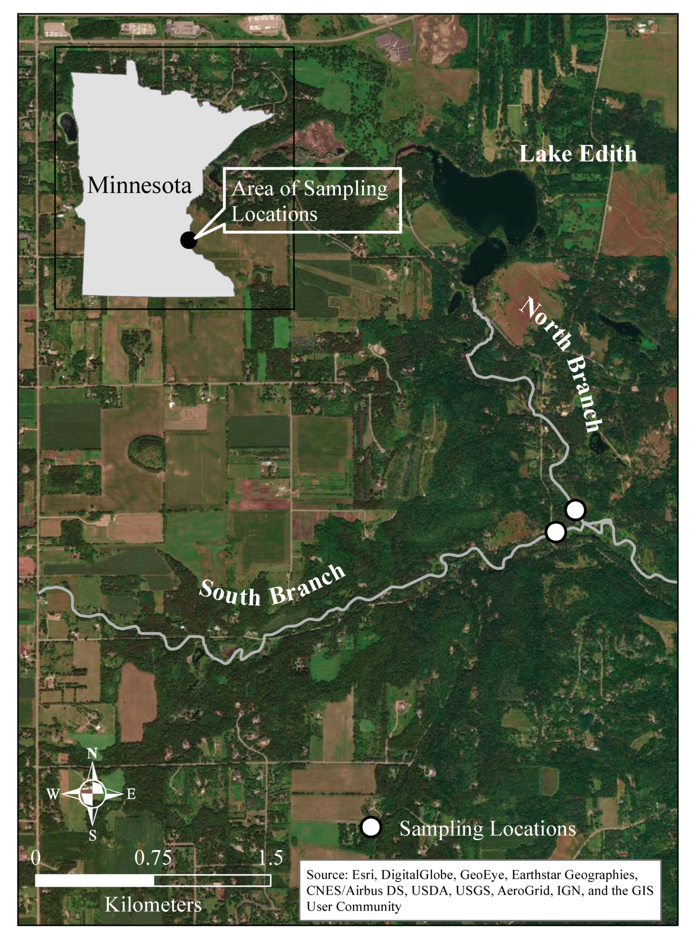
Figure 2.
Box-plots water temperature and stream discharge for two locations on Valley Creek from May–November in 2017–2019. Discharge data were unavailable for 2018 and May–June 2019.
Figure 2.
Box-plots water temperature and stream discharge for two locations on Valley Creek from May–November in 2017–2019. Discharge data were unavailable for 2018 and May–June 2019.

Figure 3.
Box-plots of light availability (photosynthetically active radiation—PAR) in an open area near the North Branch of Valley Creek, MN, and in a forested area just upstream.
Figure 3.
Box-plots of light availability (photosynthetically active radiation—PAR) in an open area near the North Branch of Valley Creek, MN, and in a forested area just upstream.
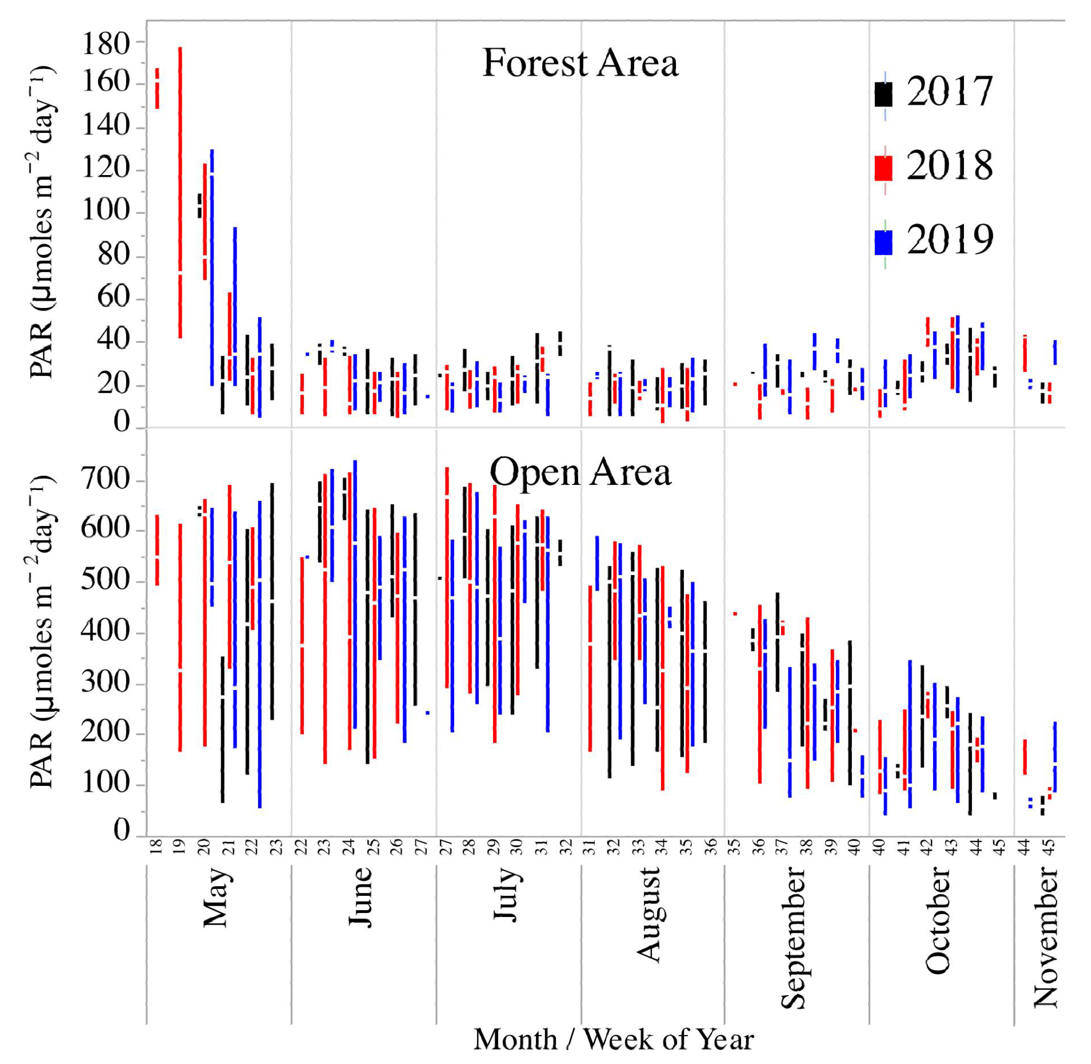
Figure 4.
Vertical hydraulic gradient (delta H) in two branches of Valley Creek, MN. The North Branch is a gaining stream and the South Branch is a losing stream.
Figure 4.
Vertical hydraulic gradient (delta H) in two branches of Valley Creek, MN. The North Branch is a gaining stream and the South Branch is a losing stream.

Figure 5.
Box-plots of dissolved oxygen (% saturation) for two locations on Valley Creek from May to November in 2017–2019. Letters show years that were significantly different based on a mixed-model ANOVA.
Figure 5.
Box-plots of dissolved oxygen (% saturation) for two locations on Valley Creek from May to November in 2017–2019. Letters show years that were significantly different based on a mixed-model ANOVA.

Figure 6.
Box-plots of GPP, ER, and NEP for the North and South Branches of Valley Creek, MN. Values with the same letter are not significantly different based on mixed-model ANOVAs on ln-transformed data and a significant interaction term between year and location.
Figure 6.
Box-plots of GPP, ER, and NEP for the North and South Branches of Valley Creek, MN. Values with the same letter are not significantly different based on mixed-model ANOVAs on ln-transformed data and a significant interaction term between year and location.

Figure 7.
Relationship between water temperature or photosynthetically active radiation (PAR) on measures of ecosystem metabolism—GPP, ER, and NEP. Lines are best-fit lines, and shaded areas are 95% confidence limits.
Figure 7.
Relationship between water temperature or photosynthetically active radiation (PAR) on measures of ecosystem metabolism—GPP, ER, and NEP. Lines are best-fit lines, and shaded areas are 95% confidence limits.

Figure 8.
Effect of stream discharge on various measures of ecosystem metabolism (GPP, ER, and NEP). Lines are parametric best-fit lines, and shaded areas are 95% confidence limits.
Figure 8.
Effect of stream discharge on various measures of ecosystem metabolism (GPP, ER, and NEP). Lines are parametric best-fit lines, and shaded areas are 95% confidence limits.


Table 1.
Physical and chemical parameters for the North and South Branches of Valley Creek, Minnesota. Values are least mean squares from mixed-model ANOVAs except for P and N, where values are means. Values in parentheses are standard errors except for N and P, where the values are standard deviations.
| Parameter | North Branch | South Branch | ||||
|---|---|---|---|---|---|---|
| 2017 | 2018 | 2019 | 2017 | 2018 | 2019 | |
| Depth (m) | 0.33 a (0.001) | 0.19 b (0.001) | 0.35 c (0.001) | 0.29 d (0.001) | 0.27 e (0.001) | 0.37 f (0.001) |
| Discharge (m3 s−1) 1 | 0.23 a (0.001) | — | 0.21 b (0.002) | 0.27 c (0.001) | — | 0.26 d (0.001) |
| Temperature (°C) 2 | 17.6 a (0.21) | 17.7 b (0.21) | 17.2 c (0.21) | 11.3 d (0.21) | 11.6 e (0.21) | 11.1 f (0.21) |
| Dissolved oxygen (% saturation) 2 | 95.5 a (0.05) | 93.5 b (0.06) | 93.0 c (0.06) | 96.3 d (0.05) | 96.8 e (0.04) | 95.1 f (0.05) |
| Conductivity (µS cm−1) 2 | 451.0 a (2.0) | — | — | 436.6 b (2.0) | 427.9 (0.1) | — |
| Dissolved P (μg L−1) 3 | 11.3 a (2.7) | 18.2 a (9.3) | 11.6 a (3.1) | 10.0 a (0.7) | 12.6 a (0.1) | 14.1 a (5.7) |
| Dissolved N (mg L−1) 3 | 2.75 a (0.99) | 2.9 a (0.92) | 2.79 a (0.79) | 8.34 b (0.25) | 9.28 b (0.21) | 9.78 b (0.46) |
1. Mean for dates in 2017–2019 when data were available for both streams. 2. Mean during the period of study. 3. Data from Washington County Conservation District and the St. Croix Watershed Research Station. Values with the same letter are not significantly different.
Table 2.
Mixed-model ANOVAs of location and year on water temperature, water depth, arcsine-transformed percent dissolved O2 (DO), and measures of ecosystem metabolism—ln (gross primary production—GPP), ln (ecosystem respiration—ER), and ln (net ecosystem production—NEP).
Table 2.
Mixed-model ANOVAs of location and year on water temperature, water depth, arcsine-transformed percent dissolved O2 (DO), and measures of ecosystem metabolism—ln (gross primary production—GPP), ln (ecosystem respiration—ER), and ln (net ecosystem production—NEP).
| Variable | Factor | F Ratio | Degrees of Freedom | Probability > F |
|---|---|---|---|---|
| Water depth | Year | 128,744.2 | 2, 154,114 | <0.0001 |
| Location | 10,356.5 | 1, 154,097 | <0.0001 | |
| Year * Location | 25,347.5 | 2, 154,083 | <0.0001 | |
| Discharge | Year | 188.4 | 1, 690 | <0.0001 |
| Location | 1445.9 | 1, 1446 | <0.0001 | |
| Year * Location | 9.3 | 1, 573 | 0.002 | |
| Temperature | Year | 599.8 | 2, 148,717 | <0.0001 |
| Location | 311,070.6 | 1, 311,070 | <0.0001 | |
| Year * Location | 56.5 | 2, 148,707 | <0.0001 | |
| % DO | Year | 5143.7 | 2, 125,124 | <0.0001 |
| Location | 21,036.5 | 1, 125,129 | <0.0001 | |
| Year * Location | 2807.5 | 2, 125,066 | <0.0001 | |
| GPP | Year | 12.8 | 2, 809 | <0.0001 |
| Location | 578.2 | 1, 808 | <0.0001 | |
| Year * Location | 23.5 | 2, 795 | <0.0001 | |
| ER | Year | 38.0 | 2, 844 | <0.0001 |
| Location | 1.3 | 1, 845 | 0.3 | |
| Year * Location | 67.0 | 2, 832 | <0.0001 | |
| NEP | Year | 5.4 | 2, 855 | 0.0046 |
| Location | 128.6 | 1, 859 | <0.0001 | |
| Year * Location | 33.9 | 2, 846 | <0.0001 |
Table 3.
Summary of mean GPP, ER, and NEP for the two locations and each of the years of the study. Values in parentheses are standard deviations. Values with the same letter are not significantly different based on mixed-model ANOVAs on ln-transformed data and a significant interaction term between year and location. Bolded values are maximum values, and those in italics are minimum values.
| Variable | Year | |||||
|---|---|---|---|---|---|---|
| 2017 | 2018 | 2019 | ||||
| North Branch | South Branch | North Branch | South Branch | North Branch | South Branch | |
| GPP | 1.3 (1.4) a | 3.6 (1.9) c | 1.6 (2.2) a | 10.5 (17.0) d | 3.0 (1.5) b | 5.5 (3.6) c |
| ER | 13.8 (6.1) a,b | 10.8 (4.7) b,c | 17.9 (9.5) a | 12.9 (16.6) c | 5.6 (8.1) d | 12.6 (5.8) b,c |
| NEP | −12.5 (5.9) a | −7.2 (4.2) c | −16.3 (9.3) b | −2.4 (3.3) d | −2.7 (8.8) a,c | −7.1 (5.7) c |
Table 4.
ANCOVAs of ln(water temperature) on ln(GPP), ln(ER), and ln(NEP) for the North Branch and South Branch of Valley Creek, MN.
Table 4.
ANCOVAs of ln(water temperature) on ln(GPP), ln(ER), and ln(NEP) for the North Branch and South Branch of Valley Creek, MN.
| Variable | Factor | F Ratio | Degrees of Freedom | Probability > F |
|---|---|---|---|---|
| GPP | ln (temperature) | 15.5 | 1, 868 | <0.0001 |
| Location | 97.8 | 1, 868 | <0.0001 | |
| ln (temperature) * location | 0.5 | 1, 868 | 0.47 | |
| ER | ln (temperature) | 3.5 | 1, 868 | 0.06 |
| Location | 0.7 | 1, 868 | 0.4 | |
| ln (temperature) * location | 22.9 | 1, 868 | <0.0001 | |
| NEP | ln (temperature) | 3.5 | 1, 868 | 0.06 |
| Location | 75.3 | 1, 868 | <0.0001 | |
| ln (temperature) * location | 22.9 | 1, 868 | <0.0001 |
Table 5.
ANCOVA of ln(PAR) on ln(GPP), ln(ER), and ln(NEP) for the North Branch and South Branch of Valley Creek, MN.
Table 5.
ANCOVA of ln(PAR) on ln(GPP), ln(ER), and ln(NEP) for the North Branch and South Branch of Valley Creek, MN.
| Variable | Factor | F Ratio | Degrees of Freedom | Probability > F |
|---|---|---|---|---|
| GPP | ln (PAR) | 45.0 | 1, 868 | <0.0001 |
| Location | 83.1 | 1, 868 | <0.0001 | |
| ln (PAR) * location | 32.9 | 1, 868 | <0.0001 | |
| ER | ln (PAR) | 0.1 | 1, 868 | 0.8 |
| Location | 3.9 | 1, 868 | 0.05 | |
| ln (PAR) * location | 29.3 | 1, 868 | <0.0001 | |
| NEP | ln (PAR) | 0.6 | 1, 868 | 0.4 |
| Location | 107.2 | 1, 868 | <0.0001 | |
| ln (PAR) * location | 28.4 | 1, 868 | <0.0001 |
Publisher’s Note: MDPI stays neutral with regard to jurisdictional claims in published maps and institutional affiliations. |
© 2021 by the author. Licensee MDPI, Basel, Switzerland. This article is an open access article distributed under the terms and conditions of the Creative Commons Attribution (CC BY) license (http://creativecommons.org/licenses/by/4.0/).
Share and Cite
MDPI and ACS Style
Hornbach, D.J. Multi-Year Monitoring of Ecosystem Metabolism in Two Branches of a Cold-Water Stream. Environments 2021, 8, 19. https://0-doi-org.brum.beds.ac.uk/10.3390/environments8030019
AMA Style
Hornbach DJ. Multi-Year Monitoring of Ecosystem Metabolism in Two Branches of a Cold-Water Stream. Environments. 2021; 8(3):19. https://0-doi-org.brum.beds.ac.uk/10.3390/environments8030019
Chicago/Turabian StyleHornbach, Daniel J. 2021. "Multi-Year Monitoring of Ecosystem Metabolism in Two Branches of a Cold-Water Stream" Environments 8, no. 3: 19. https://0-doi-org.brum.beds.ac.uk/10.3390/environments8030019
Note that from the first issue of 2016, this journal uses article numbers instead of page numbers. See further details here.