Article

Leaf-Level Spectroscopy for Analysis of Invasive Pest Impact on Trees in a Stressed Environment: An Example Using Emerald Ash Borer (Agrilus planipennis Fairmaire) in Ash Trees (Fraxinus spp.), Kansas, USA

by
Laura M. Moley
1,*,
Douglas G. Goodin
1 and
William P. Winslow
2
1
Department of Geography and Geospatial Sciences, Kansas State University, Manhattan, KS 66503, USA
2
Department of Landscape Architecture and Urban Planning, Texas A & M University, College Station, TX 77843, USA
*
Author to whom correspondence should be addressed.
Submission received: 10 February 2022 / Revised: 8 March 2022 / Accepted: 8 March 2022 / Published: 24 March 2022

Abstract

:
The most visible symptoms of emerald ash borer (EAB) (Argilus planipennis Fairmaire) infestation do not usually appear until six years after the borer’s arrival, by which time the prognosis is so grim that many communities have resorted to either heavy chemical use that only slows mortality, or clear-cutting the entire ash tree population. We utilized leaf-level spectroscopy for early detection of invasive pest-related stress, focusing on EAB as it reaches the edges of the geographic range for green and white ash trees (Fraxinus pennsylvanica and Fraxinus americana) in North America. Over the course of two full growing seasons, we sampled trees in three study areas with EAB infestation in Johnson County, Kansas, and two sample groups without infestation in Riley County, Kansas. Our method utilizes field spectrometer readings for reflectance, along with lab spectrophotometry for estimation of leaf chlorophyll and carotenoid content at several points during the growing season. Results show significant differences between pigment ratios and hyperspectral indicators between infested and non-infested ash trees, although the extent of the separation varies across the foliar season. This work has the potential to make stress diagnosis more effective, thereby improving response, and decreasing both chemical application and plant loss.

1. Introduction

The most visible symptoms of emerald ash borer (EAB) infestation do not usually appear until six years after the borer’s arrival, by which time the prognosis is so grim that many communities have resorted to either heavy chemical use that only slows mortality, or clear-cutting the entire ash tree population [1]. Native to Asia, the emerald ash borer (Agrilus planipennis Fairmaire) is believed to have arrived in North America during the mid-1990s, but was first identified in southeastern Michigan in 2002 [2]. While North America is home to several species of native borers that are generally tolerated by ash trees without serious harm, the invasive emerald ash borer causes nearly 100% mortality in affected ash populations if left untreated or treated late in the progression.
The adult insect, approximately 8.5 to 12.5 mm in length and bright green in color, bores into the tree and lays eggs in the cambium [3]. After hatching, the larvae eat their way through the phloem and xylem, eventually tunneling around the tree, under the bark, creating a girdling effect that slowly cuts off the flow of moisture and nutrients to higher portions of the tree [1]. Small D-shaped bore holes in the already rough and grooved ash bark can be difficult to see, and the larval tunneling is only visible where bark has been removed or has fallen off. Unless they are actively searching, homeowners, community foresters, and park managers may not notice signs of infestation until they begin to see bare branches and unexpected loss of leaves.
As upper branches are deprived of water and nutrients, they become defoliated and over time large sections of the crown may be devoid of leaves during the regular growing season. The shape and structure of the crown are noticeably altered, and in urban and suburban areas, bare branches are often removed through pruning, which further changes the morphology of the crown. Lower on the tree, especially on the upper trunk and main limbs, where the flow of nutrition and moisture is still active, many infested trees begin to sprout epicormic branches, which are typically bright green and may grow unusually large leaves in comparison with the rest of the tree. These later symptoms are readily apparent and easily identified, but because they result from significant, irreversible damage to the tree’s internal transport system, it is generally too late to save the tree by the time they appear.
North America is home to six native species of Ash trees, and the natural geographic ranges for two of these—green ash (Fraxinus pennsylvanica Marshall), and white ash (F. americana L.)—reach parts of Kansas (Figure 1). Due to its position near the edge of the trees’ ranges, the study area for this project represents a transition zone where the trees experience multiple sources of environmental stress [4,5]. Many of these trees are already stressed from heat, irregular soil moisture, and endemic fungi, along with the stress associated with an urban environment. Ash populations in this region contain a few examples of natural growth, primarily in riparian areas, but consist mostly of intentionally planted individuals in human-built landscapes. Both green and white ash are hybridized for landscape use, which may complicate the genetics of the natural plants and potentially impact their response to infestation.
With their upright, roughly symmetrical form, and classic round shape, ash trees are frequently used as ornamental and shade trees in landscape design. Following the rapid spread of Dutch elm disease in the 1970s, ash trees were increasingly put into service as an alternative in creating a tree-lined street aesthetic in suburban residential areas throughout the northeastern and middle-western United States. This created a visual shift from the over-arching canopy above residential streets in older, inner-ring suburbs, to the rounded crowns of foliage lining suburban neighborhoods built in the 1980s and 1990s. Since the early 2000s, EAB infestation has contributed to a loss of suburban trees, similar to that caused by Dutch elm disease, and another shift in the landscape aesthetic.
In northeast Kansas, the emerald ash borer was first identified in counties bordering Missouri, and the USDA officially confirmed an infestation in Johnson County, Kansas, at a commercial landfill site in July 2013 (Figure 2). Trees at the facility were believed to have been infested by insects carried in with waste materials from neighboring states. The Johnson County Parks and Recreation Department (JCPRD) quickly identified additional affected trees in the area. With EAB infestation already established and spreading, parks officials, neighboring municipalities, and homeowners’ associations then had limited options for combatting the infestation and preserving their trees. Monitoring began in counties farther west, in an effort to identify any additional areas of infestation at an earlier stage.
All of the study sites lie within the transitional region between the Eastern Temperate and Great Plains ecoregions, characterized by a continental temperature regime and highly variable inter-annual precipitation [6]. Monthly temperature and precipitation values for the three observation stations closest to the collection sites are summarized in Table 1. Temperature values are similar across all study sites, and show consistent patterns across time in both of the study years. The precipitation values do show evidence of an east-west gradient; however, this variation occurs within the context of within-year inter-site variability that is of similar magnitude. In general, climate conditions across the sites are similar, and they vary considerably from those within the core ranges of both species.
The environmental challenges of weather and climate conditions near the edges of the trees’ natural range are compounded by the fact that all of the trees in our samples are subjected to urban and suburban growing conditions. Particulate matter from industrial and motor vehicle exhaust creates a continual impact on air quality, contributing to surface and ground water contamination, and soil pollution. Extensive pavement (including vast suburban parking lots) increases soil temperature through heat retention, creates a physical barrier to plant growth and moisture infiltration, and leads to contaminated runoff that is often high in heavy metal content.
In addition to stresses associated with heat, irregular soil moisture, and urban growing conditions, both green and white ash trees in our study areas are subject to the impact of endemic fungi, especially mycosphaerella spp., which causes brown leaf spots and decreased photosynthetic activity beginning in mid to late summer, often followed by earlier than normal senescence. Some evidence of fungal activity was present in all sample groups and in each collection year, but it is most prevalent in years with higher moisture levels early in the season, as well as in areas with significant leaf litter remaining on the ground. These multiple stressors can make it more difficult to identify the specific causes for apparent decline in the health of ash trees, and may also cause greater vulnerability to the effects of EAB infestation for trees whose vitality is already compromised.
Spectral analysis has been applied to the challenging problem of non-invasive detection of EAB, with promising results [7,8,9]. Though encouraging, these results have generally been based on spectral observations of the entire tree canopy, using hyperspectral airborne instruments, or field-portable spectrometers deployed in situ and at close proximity to the canopy. Under these conditions, the signal received by the remote sensing instrument combines leaf level reflectance (driven by pigment, water content, and cell structure at the leaf level) see [10], with reflected signal resulting from variations in crown composition and morphology due to the presence of the pest. In some trees (for example, those that have been maintained in a way that alters their canopy shape and composition), the latter components may be less prominent and therefore less apt to serve as diagnostic indicators. Previous efforts have also been made to apply information about the spatial context of potentially infested trees as a diagnostic element e.g., [7]. However, such data may not always be readily available to incorporate into a detection effort. In situations such as these, it may be necessary to rely only on leaf-level reflectance, raising the question of whether such determinations can be made adequately based only on spectral reflectance data [11].
Previous analyses of EAB also generally have collected data from only a single time during the growing season, whereas the factors that control leaf and canopy spectral response (crown structure, leaf age, photochemical concentrations) can vary across a growing season, and may affect spectral reflectance [12]. Such spectral variations may in turn influence the ability of sensors to detect the effects of EAB. In addition, the majority of previous analyses were done using trees located within the interior of the ash species’ range in North America (see Figure 1), under conditions more conducive to their growth and development, meaning that the invasive pest was often the primary environmental stress facing the trees. At locations such as ours, more peripheral to the distribution of ash, environmental challenges imposed by ecoregion and climatic regime (especially temperature and moisture availability) impose additional organism-level stresses that further influence or alter signals associated with EAB presence.
The difficulties associated with detection and identification of EAB infestation (especially when the onset of infestation is recent or when trees are dispersed over an extensive spatial area) have resulted in widespread interest in the use of remote sensing to identify and map the locations of affected trees. Applications of remote sensing to EAB detection have used hyperspectral reflectance data, in order to provide a more detailed reflectance spectrum of leaf and canopy elements, and high spatial resolution imagery capable of resolving potentially infested trees as individuals or in small clusters [7,8,13,14]. Typical spectra from infested and non-infested trees (Figure 3) illustrate some distinguishing spectral features. Infested trees tend to absorb less (and thus reflect more) blue and red light, which occur in the electromagnetic spectrum between wavelengths of 400 and 500 nm, and between 600 and 700 nm, respectively. Conversely, infested trees absorb more (and reflect less) light in the green spectral region, between 500 and 600 nm.
Even with the use of detailed spectra, such as those shown in Figure 3, the differences in spectral reflectance between the leaves of infested and non-infested trees are subtle, and sometimes difficult to distinguish. This lack of pronounced distinguishing features at the leaf level has led researchers to make use of remote observations at the canopy level, integrating reflectance features representing both foliar properties (i.e., internal leaf structure and pigment content), and canopy properties (branch and leaf composition and distribution). However, ash trees in built and managed landscapes such as parks, suburban residential streets, or parking lots are often maintained for aesthetic quality, resulting in canopies in which common visual indicators of an infested tree, such as twig and branch dieback, epicormic branching, and canopy asymmetry are no longer as apparent [8]. In situations such as these, available remotely sensed information might by necessity be reduced to those reflectance features associated with the leaves themselves, possibly complicating the use of such information for detection of EAB symptoms in individual ash trees.
In order to understand how the effects of EAB infestation and other systemic organism-level stressors might affect the leaf-level spectral response of ash trees, it is necessary to consider how organism-level stress is related to the photochemical and photosynthetic systems of the trees, and how these systems control the patterns of absorption and reflectance across the visible and infrared regions of the spectrum. Previous research has shown that EAB infestation affects the concentration of photochemical pigments in infested ash trees [7]. Investigating pigment dynamics in Fraxinus trees with various states of infestation (including non-infested) is, therefore, a promising avenue for linking the physiological effects of infestation to the reflectance response.
Photochemical processes in any vegetative organisms, include trees, are controlled by a number of light-activated pigments. These include chlorophyll (occurring as two types, Chl-a and Chl-b), the primary light-harvesting pigment of the photosynthesis process, as well as a number of additional photochemical pigments, such as carotenoids, which aid in the photosynthetic process by absorbing light at shorter wavelengths and helping to dissipate excess heat energy [15]. Variations in the relative contents of these pigments have been shown to be an indicator of the physiological and phenological status of various plant types [16,17,18], and thus can be used as photochemical indicators of stress. In particular, the ratio of chlorophyll-a to chlorophyll-b (Chl a/b), and the ratio of total Carotenoids to total chlorophyll (Car/Chl) are widely used indices of plant physiological status, phenological state, and environmental stress [19,20,21,22].
In addition to their role as physiological status indicators, photochemical pigments are the link between plant state and leaf/canopy reflectance, and therefore to the remote sensing of plant photochemical processes [23,24]. chlorophyll -a and -b both show a distinctive pattern of absorption and reflectance in the visible part of the electromagnetic spectrum between 400 and 700 nm. Between 400 and 500 nm, (blue light) and 600 and 700 nm (red light) electromagnetic energy is absorbed, while between 500 and 600 nm, more light is reflected. The result of this pattern is photosynthesizing vegetation appearing green to the unaided human eye. At wavelengths beyond 700 nm (corresponding to the near infrared region of the spectrum), photosynthesizing plants are strong reflectors of light, resulting in steep transition in the reflectance curve [25,26] (see Figure 3). Carotenoids also absorb visible light, although their absorption is less pronounced, and occurs in a narrower range of the spectrum between 460 nm and 550 nm (Figure 3). The overlap in their spectra complicates direct analysis via remotely sensed spectral reflectance [16], but absorption by these pigments in the visible spectrum makes them useful for analysis by spectroscopic methods.
This study seeks to identify methods for evaluating the spectral and pigmentary impact of EAB infestation at the leaf level, to facilitate diagnosis prior to the onset of more visible late-stage symptoms, and improve response options for communities. In built landscapes, ash trees diagnosed with EAB infestation are often treated with systemic insecticides, such as emamectin benzoate. Treatment of EAB in ash trees differs from methods for addressing corn borers and similar infestations affecting crops [27,28,29], in that damage to the trees takes place over a period of years and is irreversible. Such interventions are less effective in preserving the tree when infestation is more advanced, since they cannot repair the damage already done [30]. The treated trees we sampled belonged to, and were treated by, the Johnson County Parks and Recreation Department, who utilized a protocol of injecting infested trees once every two years in order to maintain a consistent level of insecticide within the tree (Shafer, C., Johnson County Parks and Recreation Department, Personal Communication). This treatment method is lethal to EAB within the tree (eggs, larvae, and adults), but does not directly affect the photoactive pigments in the leaves themselves. The treatment does indirectly impact photosynthesis by reducing any additional stress imposed on the tree by the pest [31].
The important goals of this current research are therefore, (1) to investigate pigment content and spectral reflectance from ash trees at the leaf level, at multiple times throughout the foliated period, and (2) to compare untreated EAB infested ash trees, infested trees treated with systemic insecticides, non-infested individuals in a compromised condition due to other sources of stress, and healthy, non-infested trees. This work addresses two key questions. First, can groups of Fraxinus trees with differing states of infestation and general health be differentiated based on photochemical pigment content and leaf-level spectral reflectance? Second, does the ability to differentiate vary during the growing season, and if so, what are the optimal times for measurement?

2. Materials and Methods

Based on preliminary site surveys conducted in 2016, we identified five groups of trees, with each group consisting of a mix of green ash (Fraxinus pennsylvanica Marshall), and white ash (F. americana L.), with varying infestation and stress conditions. A total of three of the sites were located in Johnson County, Kansas, a suburban area west of Kansas City, Missouri. EAB was identified in Johnson County in 2013, and therefore all three were classified as infested sites. These sites included a transect of trees along a residential street in Shawnee, Kansas, near where EAB was first identified in Johnson County. The trees in this group were clearly infested, showing many of the visible signs of EAB presence (e.g., crown dieback, epicormal branching, and, in some cases, visible larvae damage beneath the bark). A second sampling site was established at Mid-America Sports Complex, a Johnson County park department facility with infested ash trees currently being treated with chemical insecticide. The trees in this sample received (in addition to treatment) routine pruning and maintenance, thus they showed fewer outward signs of EAB damage. The third sampling site, located at Heritage Park in southern Johnson County (further from the origin of the infestation), consisted of trees in earlier stages of EAB damage and initially represented a mixture of treated and untreated, infested trees. As our research continued, more of the trees were treated by the park manager as their condition began to show visible signs of deterioration.
An important facet of this project is its comparison of treated and untreated infested trees, with non-infested trees in a similar environment. In order to be certain that a comparative sample area would have ash trees that were definitely not EAB infested, we established two more collection sites in Riley County, Kansas (Figure 2), where monitoring has so far (as of February 2022) indicated no EAB presence in the area (Bomberger, K, Kansas Department of Forestry, Personal Communication). Ash trees in our Riley County samples included a group of non-infested, mature trees in relatively healthy condition, growing in less stressed locations on the grounds of Kansas State University (which is maintained as a public arboretum) and in the surrounding neighborhoods; and a second group of more stressed non-infested individuals, also located on the KSU campus, but mostly growing in and around parking lots and planted in medians. This second group was added in order to compare non-infested trees in poorer overall condition with trees known to be in poor shape due to EAB presence. As of early 2022, no EAB infestation had been identified in Riley County, but over the course of this research, intervening counties as far west as Topeka in Shawnee County have had EAB confirmation (Figure 2). While the Riley and Johnson County sites were separated by over 100 km, the environmental differences between them were not pronounced enough to interfere with a comparison (see Table 1).
Samples were collected from each of the five sample site groups described above, at four times during each of the growing seasons. Sampling dates were selected to correspond to four general stages in the foliar season: (1) early leaf stage, (2) mature leaf stage, (3) peak greenness, and (4) late leaf stage. Each of these stages represents variation in the age of the leaf (which affects its internal optical properties) see [12], and tree physiology (e.g., nutrient or water stress). Weather conditions and seasonal differences precluded exact replication of the sampling dates between the two years, but efforts were instead made to sample at times consistent with the four stages listed above. Sample dates and sizes for each site are summarized in Table 2. To the extent possible, the same trees were sampled during each data collection; however, this was not always feasible since some trees died or were removed during the study period. Trees lost from the sample groups were replaced with others from the same area and conforming to the same conditions.
Sample leaves used for pigment and spectral analysis were collected from a random mid-canopy location within each of the sampled trees using a telescoping pruner, temporarily stored in a cool and dark container, then transported to the lab for further analysis. Spectral reflectance curves were collected from the adaxial surface of the terminal leaflet of each sample using an ASD-FR spectrometer equipped with a leaf clip with internal light source. After the spectral sample was collected, a 0.6 cm circular punch sample of leaf tissue was excised from the sample and stored at −18 °C until pigment analysis could be done. Pigment analysis consisted of immersing each punch sample in 5 mL of dimethyl sulfoxide (DMSO) for 72 h in darkness at room temperature. The resulting solution was then analyzed for concentration per unit area of chlorophyll-a, chlorophyll-b, and total carotenoids using a Cole-Parmer 1200 spectrophotometer. Extraction equations were from Wellburn [32].
The principal questions guiding this research were whether leaf pigment content could be used to differentiate ash trees in a number of EAB infestation statuses, and, if so, whether spectral indices related to pigment content could also be used for this purpose. The first step in addressing these questions was to establish the relationship between pigment contents and a set of selected spectral indices. To quantify pigment content, we used two pigment ratios shown to be indicators of general organismic stress in photosynthetic plants. The ratio of chlorophyll-a to chlorophyll-b (Chl a/b) has been shown to respond to a number of biotic and abiotic stresses, including water and nutrient stress [33]. Since the infestation process of EAB disrupts transfer of water nutrient resources within the tree, the Chl a/b ratio seemed a promising one to investigate. We also evaluated the ratio of total carotenoids to total chlorophyll (Car/Chl), a general indicator of environmental stress and phenological state [17,18,34].
For the reflectance analysis component, we chose five potential indices to test (Table 3). These indices were selected based on evaluation of previous studies addressing EAB infestation [7,8], as well as other types of plant stress more generally [16,18,23,26]. A wide array of indices has been used for applications of this type, including ones related to canopy structure, biochemistry, and physiology [35]. The five indices were calculated from each of the ASD reflectance spectra, using the HSDAR package in R [36]. Once the various spectral indices and pigment ratios were calculated, each ratio was correlated to all five spectral indices for the entire 2017 and 2018 data set, in order to determine which of them was most closely related to the pigment data.
Following the correlation analysis, the next analytical step was to test whether pigment ratios and hyperspectral indices varied significantly between the groups of ash trees. For this analysis, the Kruskal–Wallis (K-W) test was used, with each group acting as a statistical treatment [41]. The K–W test is a non-parametric rank-based one-way test analogous to analysis of variance (ANOVA), used to determine whether multiple samples originate from the same distribution, thus it is suitable for finding significant differences and groupings within data based on specific characteristics. The K–W test is appropriate when sample sizes are too small to ensure normal distribution [42]. In cases where there were significant inter-group differences, the pair-wise Conover–Iman comparison test with the Benjamini–Hochberg adjustment was used to further determine differences between the various groups [43,44]. Analysis was performed using R with Stats [45].

3. Results

3.1. Pigment Analysis

Results of this initial correlation analysis for 2017 and 2018 are summarized in Table 4. Not surprisingly, the strongest relationships were between the pigment ratios and indices such as PRI, GMb, and CCRI, all of which incorporate spectral information specifically related to pigment absorption. PRI was the strongest correlate to the pigment ratios, which again follows from its intended purpose as an indicator of photochemical processes. The water band and NPQI indices showed little relationship with pigments. Of the two pigment indices, the Car/Chl ratio was more strongly correlated to spectral response.
Based on these initial correlation results, subsequent analyses focused only on the PRI and Car/Chl variables. Further correlation analysis showed that the relationship between PRI and Car/Chl varied across the collection periods for each year, but the r-values were significant for all collection periods (see Figure 4 and Figure 5). For 2017, the correlation values were significant for all collections, and ranged from −0.44 for earliest collection to −0.76 for the last one (Figure 4). Results from 2018 were similar, with all four time periods significantly correlated, but not to the same degree. While these results varied, they supported the use of hyperspectral indices for detecting pigment dynamics.
K–W test results for the 2017 Car-Chl data show significant differences between the sample groups in three of the four collection periods (Figure 6). Within each of the three significant collection periods, the pattern of grouping varies somewhat, but the variations suggest some coherence relative to infestation patterns. For the first (April-May) and second (June) collections, the sites where EAB is known to be present group together. In particular, the infested, treated (IT) and infested, not treated (INT) sites group together in April-May, and the two treated sites group together in June. In both cases, the other infested site forms a partially overlapping group. Grouping are less well-defined in the late-season (October) collection; however, the three infested sites continue to show some grouping, although the infested untreated and recently infested and treated groups overlap with one of the non-infested sites. The late season collection also shows the greatest differences between the less-healthy, non-infested group (NIP) and all the others. This is consistent with visual analysis of the trees, which tend to show obvious leaf fungus later in the growing season. Another noteworthy aspect of these results is the consistent separation of the two non EAB infested sites. This lack of grouping suggests that the differences between the groups are not due just to the spatial separation of the respective sites (recall that they are separated by more than 100 km), but result from physiological stresses imposed by their infestation status and landscape conditions.
The 2018 Car/Chl results (Figure 7) are similar to those from 2017. Once again, the late August-September collection did not show significant differences between the groups, although all three other collections did. EAB infested sites tended to group together, although separations between the groups were not as well-defined as in the 2017 case. In particular, the untreated infested and healthier non-infested sites overlapped with each other, which was surprising, given the difference in infestation status. In the July collection, the three EAB infested sites grouped wholly or partially with the more stressed, less healthy non-infested site. This grouping is actually consistent with conditions from that year, where visual evidence of fungus was apparent on leaves much earlier in the folial season, relative to the previous year. This result also suggests that general indices of stress, such as pigment ratios, are diagnostic of EAB infestation, but not exclusively so. As in 2017, the 2018 results from the final collection are less defined than for the previous collections, although here again the differences between the more stressed non-infested group and the other groups is most pronounced.

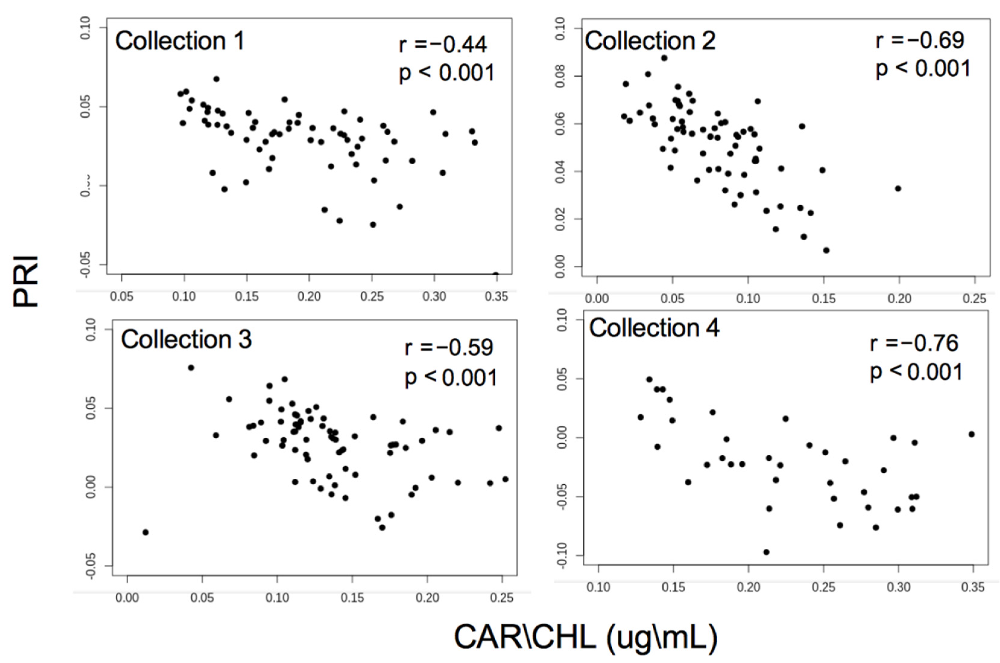
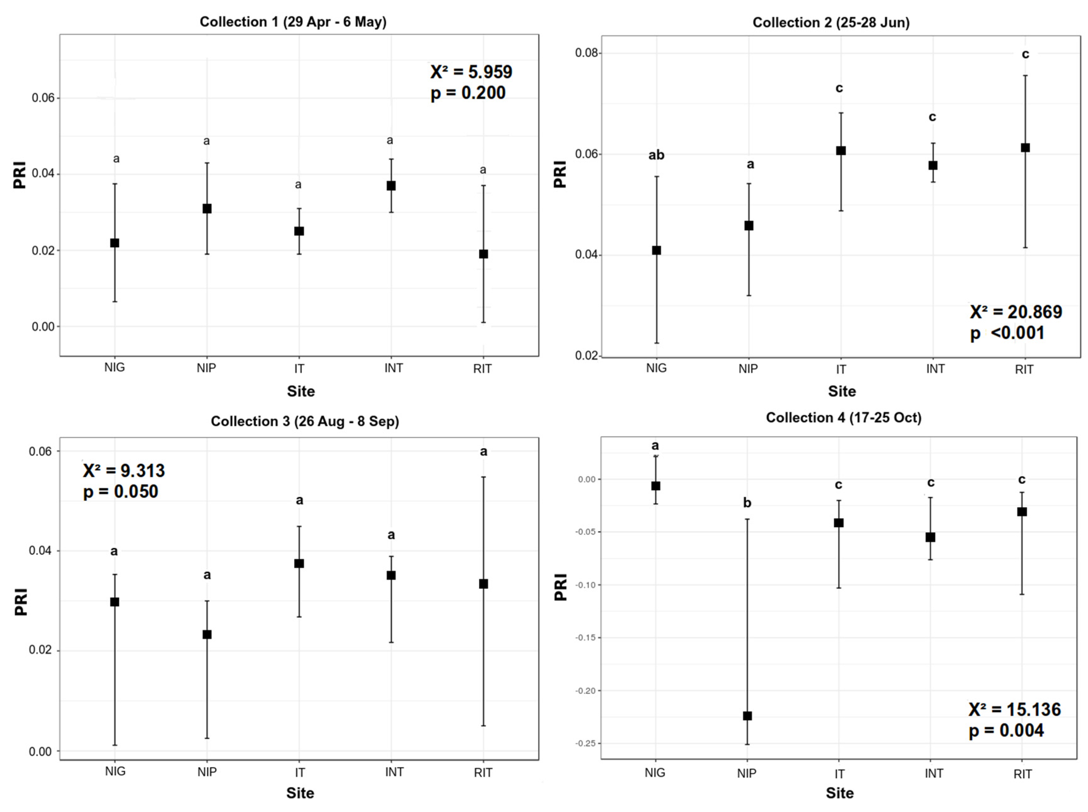
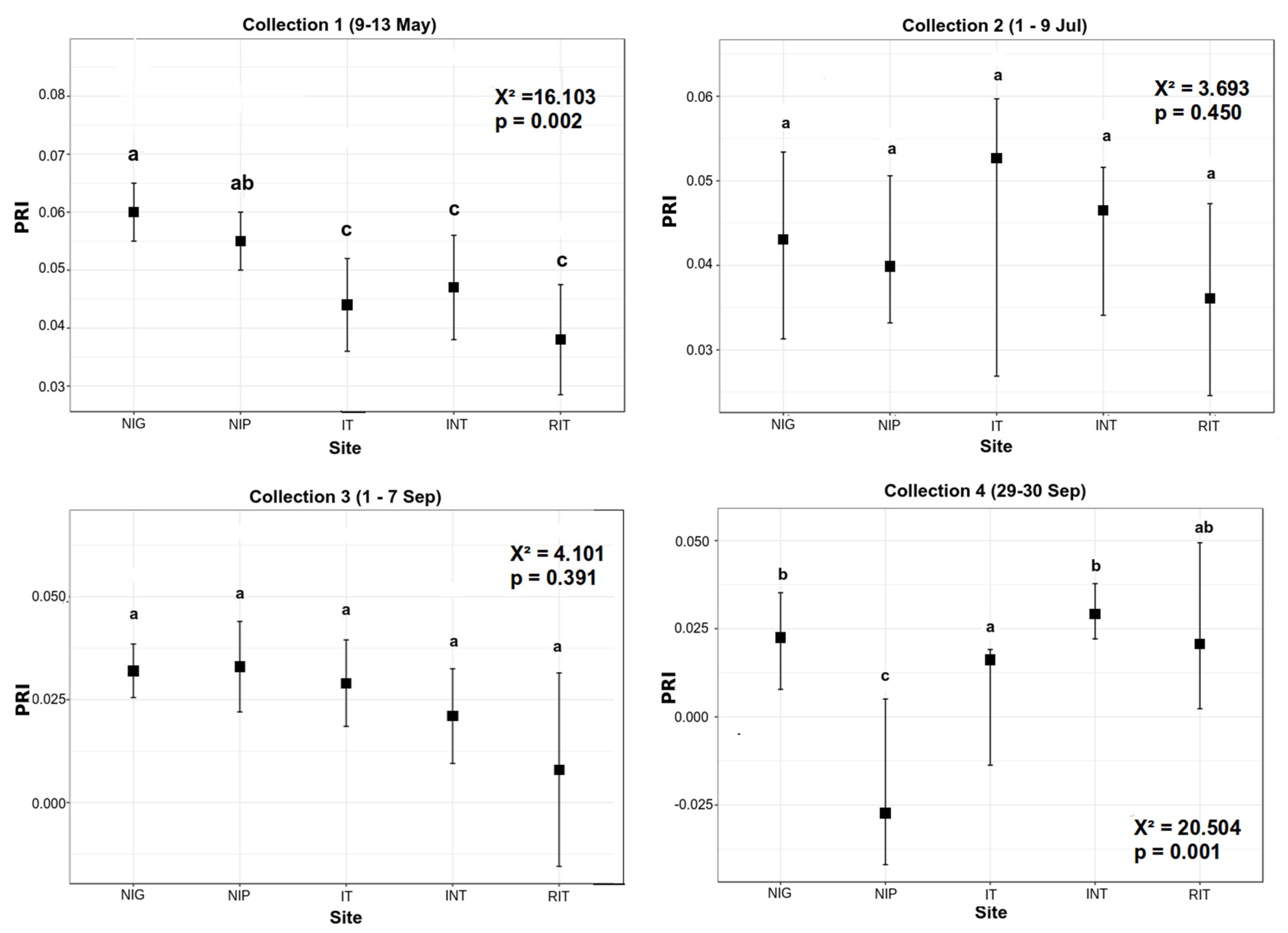
3.2. Reflectance Analysis

The K–W test results using the PRI data showed a number of similarities to the Car/Chl results, but also some noteworthy differences. As in the Car/Chl results, significant differences between the groups varied depending on collection time. Unlike the Car/Chl ratio, however, the collection periods where differences are significant or insignificant do not correspond exactly. In 2017, the June and October collections show significant differences between groups, whereas the other two do not (Figure 8). It is notable that the two collections where the K–W results were not significant correspond to the weakest correlations between PRI and Car/Chl (Figure 4). While PRI is clearly correlated with pigments (and pigment ratios), it is also influenced by other leaf properties [38], hence it is not surprising that the two metrics do not correspond exactly. In 2017, the June collection showed the most among-group difference, and again the EAB-infested sites separate either wholly or partially from the non-infested ones. In the late-season collection (October), the EAB sites continue to group together, whereas the more stressed and less stressed non-infested sites (NIP and NIG) group separately.
In 2018, the May and September collections show significant between-group separation, and the other two collections did not (Figure 9). The May results show a grouping pattern similar the one from the Car/Chl results, with the three infested sites grouping together, and the other two sites either fully or partially separated. Again, this shows that even in the presence of chemical insecticide treatment, the presence of EAB results in reflectance effects that are detectable using spectral analysis. As in the 2017 results, the more stressed non-infested site separates from the others later in the leaf-growth season, but the untreated EAB site also continues to separate, and the two treated sites form a group that partially overlaps the untreated site. These results further suggest that the PRI can provide a leaf-level diagnostic of EAB presence, but that its effectiveness varies considerably across the foliar season.
As a further test of whether the observed differences between the five treatment groups were not artifacts of the data, all of the observations were randomly assigned to five groups with sizes equaling the actual data. These randomized groups were then subjected to the Kruskal–Wallis test, using the same methods as those applied to the actual group data. This procedure was repeated twenty times, using twenty different sets of randomized data. None of these randomized trials indicated any statistically significant separation of groups, further supporting our contention that the differences in the actual groups are due to stress effects, rather than random chance.

4. Discussion

This research demonstrates significant differences in both PRI and pigment ratios between sample groups of treated and untreated EAB infested trees, and more stressed and less stressed non-infested trees. Our results show that the content of photochemical pigments varied significantly depending on whether the tree has been exposed to EAB, and whether that exposure has been chemically treated with an insecticide. This finding further reinforces the practice of using hyperspectral indices of photochemical status to detect the effects of EAB infestation (and perhaps other stressors) in potentially exposed tree populations [46]. Our results further show that among the spectral indices tested, the PRI was the most effective in differentiating, at the leaf level, among trees in various states of infestation and overall health. However, the effectiveness of PRI does seem to vary across the foliar season, and this variation may not be consistent from year to year.
Our analysis indicates that it is possible to differentiate between groups of trees with varying EAB status and environmental stress, particularly when testing occurs at useful points in leaf development. We found testing to be most helpful at early and late points in the foliar season, when specific stressors had distinct and measurable impacts. Sample measurements were least helpful during the hottest part of summer, when all groups of trees were most stressed from heat and moisture, and thus showed least differentiation from other stresses. Because the timing of these environmental conditions varies from year to year, the phase of leaf development represents a more reliable guide for timing diagnostic tests than the use of target calendar dates.
These results further show that measurements made only at the leaf-level (either pigments or reflectance) do show promise for addressing the difficult problem of identifying EAB infested trees. This finding is potentially important, since in some instances it may not be possible for managers to actually measure (remotely) the entire tree canopy in order to detect non-foliar indicators of infestation stress [47]. Such measurements require a significant infrastructure (e.g., ground-mounted instrument platforms, drones, aircraft, etc.) to support instrumentation, which may not be routinely available when and where they are needed [48]. The use of field portable or hand-held spectroradiometric devices offers a flexible and less costly way for managers to detect early evidence of infestation, without the need for imagery or extensive sampling infrastructure [49]. However, changes in the effectiveness of these leaf-level measurements across time were apparent in our results. This observation is an important finding of our study, suggesting that, while leaf-level-only diagnosis of EAB and other infestations may be possible, its effectiveness may vary considerably across time.
By measuring variations in reflectance associated with specific pigments, we determined that it is possible to detect pigmentary changes in the leaves of EAB-infested ash trees before such changes would become visible to the naked eye. For example, one of the symptoms of EAB-related decline in infested ash trees is early senescence, in which infested trees begin to show yellow leaves in the middle of the growing season—far earlier than normal autumnal senescence would usually take place. In white ash trees, whose autumn foliage color coloration would typically trend toward visible purple tones, this early senescence in infested trees is also notable for its incongruous coloration. While these pigmentary changes are visible without spectroscopy, they occur too late in the progression of the disease for any viable chance of saving the tree. Therefore, the use of spectroscopy for early detection of pigmentary changes prior to the development of visible pathology is important for improving and maintaining the health of the tree for as long as possible.
Data analysis presented here forms the basis of an early detection method for EAB infestation in stressed urban environments, with potential applications to a broader range of tree pathologies. We have conducted sampling in the subsequent foliar seasons, and the results reported here will inform analysis of these additional data. Next steps in this research will include analysis of additional pigment markers, and development of a predictive spectral model that can be adapted to canopy-level, and that could be fine-tuned to specific bands that may be diagnostic at certain points in leaf growth. Identification of a narrower spectral range for measurement would make it possible to develop lower cost detection equipment, with practical implications for environmental planning in communities facing invasive pest infestations and other environmental stressors.

5. Conclusions

From this analysis we can draw three major conclusions. First, this study demonstrates that photosynthetic pigmentation varies with EAB infestation status. In particular, the ratio of carotenoids to total chlorophyll (CAR/CHL) was most clearly diagnostic in that it most effectively differentiated between groups of trees by infestation status, and it showed the strongest correlation to spectral response. In addition, we concluded that pigmentation differences can be detected using leaf-level hyperspectral reflectance, and that the differences were most pronounced in the early and late portions of the growing season. Finally, this work established that among the indices we used, the photochemical reflectance index (PRI) was best for observing spectral differences between infestation status groups. Together, these conclusions form the basis of an early diagnostic tool, and thus, this research has the potential to make stress diagnosis more effective, thereby improving response, and decreasing both chemical application and plant loss.

Author Contributions

Conceptualization, L.M.M.; methodology, L.M.M. and D.G.G.; validation, L.M.M., D.G.G. and W.P.W.; formal analysis, L.M.M., D.G.G. and W.P.W.; investigation, L.M.M., D.G.G. and W.P.W.; resources, L.M.M., D.G.G. and W.P.W.; data curation, D.G.G.; writing—original draft preparation, L.M.M. and D.G.G.; writing—review and editing, L.M.M., D.G.G. and W.P.W.; visualization, L.M.M., D.G.G. and W.P.W.; supervision, L.M.M.; project administration, L.M.M.; funding acquisition, D.G.G. and W.P.W. All authors have read and agreed to the published version of the manuscript.

Funding

This research was funded by a University Small Research Grant from Kansas State University and the Kansas Forest Service.

Institutional Review Board Statement

Not applicable.

Informed Consent Statement

Not applicable.

Data Availability Statement

Not applicable.

Acknowledgments

The authors acknowledge the assistance of Kim Bomberger, Kansas Forest Service, and Craig Shafer, Johnson County Parks and Recreation Department.

Conflicts of Interest

The authors declare no conflict of interest.

References

  1. Herms, D.A.; McCullough, D.G. Emerald Ash Borer Invasion of North America: History, Biology, Ecology, Impacts, and Management. Annu. Rev. Entomol. 2014, 59, 13–30. [Google Scholar] [CrossRef] [PubMed] [Green Version]
  2. Haack, R.A.; Jendak, E.; Houping, L.; Marchant, K.R.; Petrice, T.R.; Poland, T.M.; Ye, H. The Emerald Ash Borer: A New Exotic Pest in North America; Newsletter of the Michigan Entomological Society: Asheville, NC, USA, 2002. [Google Scholar]
  3. Volkovitsh, M.G.; Orlova-Bienkowskaja, M.J.; Kovalev, A.V.; Bieńkowski, A.O. An Illustrated Guide to Distinguish Emerald Ash Borer (Agrilus Planipennis) from Its Congeners in Europe. For. Int. J. For. Res. 2019, 93, 316–325. [Google Scholar] [CrossRef]
  4. MacFarlane, D.W.; Meyer, S.P. Characteristics and Distribution of Potential Ash Tree Hosts for Emerald Ash Borer. For. Ecol. Manag. 2005, 213, 15–24. [Google Scholar] [CrossRef]
  5. Poland, T.M.; McCullough, D.G. Emerald Ash Borer: Invasion of the Urban Forest and the Threat to North America’s Ash Resource. J. For. 2006, 104, 118–124. [Google Scholar] [CrossRef]
  6. Omernik, J.M.; Griffith, G.E. Ecoregions of the Conterminous United States: Evolution of a Hierarchical Spatial Framework. Environ. Manag. 2014, 54, 1249–1266. [Google Scholar] [CrossRef]
  7. Zhang, K.; Hu, B.; Robinson, J. Early Detection of Emerald Ash Borer Infestation Using Multisourced Data: A Case Study in the Town of Oakville, Ontario, Canada. J. Appl. Remote Sens. 2014, 8, 1–19. [Google Scholar] [CrossRef]
  8. Pontius, J.; Martin, M.; Plourde, L.; Hallett, R. Ash Decline Assessment in Emerald Ash Borer-Infested Regions: A Test of Tree-Level, Hyperspectral Technologies. Remote Sens. Environ. 2008, 112, 2665–2676. [Google Scholar] [CrossRef]
  9. San Souci, J.; Hanou, I.; Puchalski, D. High-Resolution Remote Sensing Image Analysis for Early Detection and Response Planning for Emerald Ash Borer. Photogram. Eng. Remote Sens. 2009, 75, 905–909. [Google Scholar]
  10. Knipling, E.B. Physical and Physiological Basis for the Reflectance of Visible and Near-Infrared Radiation from Vegetation. Remote Sens. Environ. 1970, 1, 155–159. [Google Scholar] [CrossRef]
  11. Williams, D.; Bartels, D.; Sawyer, A.; Mastro, V. Application of remote sensing technology to emerald ash borer survey. In Proceedings of the 16th U.S. Department of Agriculture Interagency Research Forum on Gypsy Moth and Other Invasive Species, Annapolis, MD, USA, 18–21 January 2005. [Google Scholar]
  12. Zhang, Q.; Li, Q.; Zhang, G. Scattering Impact Analysis and Correction for Leaf Biochemical Parameter Estimation Using Vis-NIR Spectroscopy. Spectroscopy 2011, 26. Available online: https://www.spectroscopyonline.com/view/scattering-impact-analysis-and-correction-leaf-biochemical-parameter-estimation-visnir (accessed on 7 March 2022).
  13. Pontius, J.; Hanavan, R.P.; Hallett, R.A.; Cook, B.D.; Corp, L.A. High Spatial Resolution Spectral Unmixing for Mapping Ash Species across a Complex Urban Environment. Remote Sens. Environ. 2017, 199, 360–369. [Google Scholar] [CrossRef]
  14. Murfitt, J.; He, Y.; Yang, J.; Mui, A.; De Mille, K. Ash Decline Assessment in Emerald Ash Borer Infested Natural Forests Using High Spatial Resolution Images. Remote Sens. 2016, 8, 256. [Google Scholar] [CrossRef] [Green Version]
  15. Armstrong, G.A.; Hearst, J.E. Carotenoids 2: Genetics and Molecular Biology of Carotenoid Pigment Biosynthesis. FASEB J. 1996, 10, 228–237. [Google Scholar] [CrossRef] [PubMed]
  16. Carter, G.A.; Knapp, A.K. Leaf Optical Properties in Higher Plants: Linking Spectral Characteristics to Stress and Chlorophyll Concentration. Am. J. Bot. 2001, 88, 677–684. [Google Scholar] [CrossRef] [PubMed] [Green Version]
  17. Sims, D.A.; Gamon, J.A. Relationships between Leaf Pigment Content and Spectral Reflectance across a Wide Range of Species, Leaf Structures and Developmental Stages. Remote Sens. Environ. 2002, 81, 337–354. [Google Scholar] [CrossRef]
  18. Zhou, X.; Huang, W.; Zhang, J.; Kong, W.; Casa, R.; Huang, Y. A Novel Combined Spectral Index for Estimating the Ratio of Carotenoid to Chlorophyll Content to Monitor Crop Physiological and Phenological Status. Int. J. Appl. Earth Obs. Geoinf. 2019, 76, 128–142. [Google Scholar] [CrossRef]
  19. Esteban, R.; Moran, J.F.; Becerril, J.M.; García-Plazaola, J.I. Versatility of Carotenoids: An Integrated View on Diversity, Evolution, Functional Roles and Environmental Interactions. Environ. Exp. Bot. 2015, 119, 63–75. [Google Scholar] [CrossRef]
  20. Ashraf, M.; Harris, P.J. Photosynthesis under Stressful Environments: An Overview. Photosynthetica 2013, 51, 163–190. [Google Scholar] [CrossRef]
  21. Demmig-Adams, B.; Adams, W.W. The Role of Xanthophyll Cycle Carotenoids in the Protection of Photosynthesis. Trends Plant Sci. 1996, 1, 21–26. [Google Scholar] [CrossRef]
  22. Gamon, J.A.; Surfus, J.S. Assessing Leaf Pigment Content and Activity with a Reflectometer. New Phytol. 1999, 143, 105–117. [Google Scholar] [CrossRef]
  23. Blackburn, G.A. Spectral Indices for Estimating Photosynthetic Pigment Concentrations: A Test Using Senescent Tree Leaves. Int. J. Remote Sens. 1998, 19, 657–675. [Google Scholar] [CrossRef]
  24. Blackburn, G.A. Hyperspectral Remote Sensing of Plant Pigments. J. Exp. Bot. 2006, 58, 855–867. [Google Scholar] [CrossRef] [Green Version]
  25. Aronoff, S. The Absorption Spectra of Chlorophyll and Related Compounds. Chem. Rev. 1950, 47, 175–195. [Google Scholar] [CrossRef] [PubMed]
  26. Penuelas, J.; Baret, F.; Filella, I. Semi-Empirical Indices to Assess Carotenoids/Chlorophyll a Ratio from Leaf Spectral Reflectance. Photosynthetica 1995, 31, 221–230. [Google Scholar]
  27. Piesik, D.; Rochat, D.; van der Pers, J.; Marion-Poll, F. Pulsed Odors from Maize or Spinach Elicit Orientation in European Corn Borer Neonate Larvae. J. Chem. Ecol. 2009, 35, 1032–1042. [Google Scholar] [CrossRef]
  28. Piesik, D.; Rochat, D.; Delaney, K.J.; Marion-Poll, F. Orientation of European Corn Borer First Instar Larvae to Synthetic Green Leaf Volatiles: Orientation of European Corn Borer First Instar Larvae. J. Appl. Entomol. 2013, 137, 234–240. [Google Scholar] [CrossRef] [Green Version]
  29. Skoczek, A.; Piesik, D.; Wenda-Piesik, A.; Buszewski, B.; Bocianowski, J.; Wawrzyniak, M. Volatile Organic Compounds Released by Maize Following Herbivory or Insect Extract Application and Communication between Plants. J. Appl. Entomol. 2017, 141, 630–643. [Google Scholar] [CrossRef]
  30. Flower, C.E.; Dalton, J.E.; Knight, K.S.; Brikha, M.; Gonzalez-Meler, M.A. To Treat or Not to Treat: Diminishing Effectiveness of Emamectin Benzoate Tree Injections in Ash Trees Heavily Infested by Emerald Ash Borer. Urban For. Urban Green. 2015, 14, 790–795. [Google Scholar] [CrossRef] [Green Version]
  31. Hanavan, R.; Heuss, M. Physiological Response of Ash Trees, Fraxinus spp., Infested with Emerald Ash Borer, Agrilus planipennis Fairmaire (Coleoptera: Buprestidae), to Emamectin Benzoate (Tree-Äge) Stem Injections. Arboric. Urban For. 2019, 45, 132–138. [Google Scholar] [CrossRef]
  32. Wellburn, A.R. The Spectral Determination of Chlorophylls a and b, as Well as Total Carotenoids, Using Various Solvents with Spectrophotometers of Different Resolution. J. Plant Physiol. 1994, 144, 307–313. [Google Scholar] [CrossRef]
  33. Kitajima, K.; Hogan, K.P. Increases of Chlorophyll a/b Ratios during Acclimation of Tropical Woody Seedlings to Nitrogen Limitation and High Light. Plant Cell Environ. 2003, 26, 857–865. [Google Scholar] [CrossRef] [PubMed]
  34. Wolfenden, J.; Robinson, D.C.; Cape, J.N.; Paterson, I.S.; Francis, B.J.; Melhorn, H.; Wellburn, A.R. Use of Carotenoid Ratios, Ethylene Emissions and Buffer Capacities for the Early Diagnosis of Forest Decline. New Phytol. 1988, 109, 85–95. [Google Scholar] [CrossRef]
  35. Roberts, D.; Roth, K.; Perroy, R. Hyperspectral vegetation indices. In Hyperspectral Remote Sensing of Vegetation; CRC Press: Boca Raton, FL, USA, 2011; pp. 309–328. ISBN 978-1-4398-4537-0. [Google Scholar]
  36. Lehnert, L.W.; Meyer, H.; Obermeier, W.A.; Silva, B.; Regeling, B.; Bendix, J. Hyperspectral Data Analysis in R: The Hsdar Package. J. Stat. Softw. 2019, 89, 1–23. [Google Scholar] [CrossRef] [Green Version]
  37. Penuelas, J.; Fillela, I.; Biel, C.; Serrano, L.; Save, R. The Reflectance at the 950–970 Nm Region as an Indicator of Plant Water Status. Int. J. Remote Sens. 1993, 14, 1887–1905. [Google Scholar] [CrossRef]
  38. Gitelson, A.; Merzlyak, M.N. Quantitative Estimation of Chlorophyll-a Using Reflectance Spectra: Experiments with Autumn Chestnut and Maple Leaves. J. Photochem. Photobiol. B 1994, 22, 247–252. [Google Scholar] [CrossRef]
  39. Barnes, J.D.; Balaguer, L.; Manrique, E.; Elvira, S.; Davison, A.W. A Reappraisal of the Use of DMSO for the Extraction and Determination of Chlorophylls a and b in Lichens and Higher Plants. Environ. Exp. Bot. 1992, 32, 85–100. [Google Scholar] [CrossRef]
  40. Gamon, J.; Serrano, L.; Surfus, J.S. The Photochemical Reflectance Index: An Optical Indicator of Photosynthetic Radiation Use Efficiency across Species, Functional Types, and Nutrient Levels. Oecologia 1997, 112, 492–501. [Google Scholar] [CrossRef] [PubMed]
  41. Kruskal, W.H.; Wallis, W.A. Use of Ranks in One-Criterion Variance Analysis. J. Am. Stat. Assoc. 1952, 47, 583–621. [Google Scholar] [CrossRef]
  42. Daniel, W.W. Applied Nonparametric Statistics, 2nd ed.; PWS-Kent: Boston, MA, USA, 1990. [Google Scholar]
  43. Benjamini, Y.; Hochberg, Y. Controlling the False Discovery Rate: A Practical and Powerful Approach to Multiple Testing. J. R. Stat. 1995, 57, 289–300. [Google Scholar]
  44. Conover, W.J. Practical Nonparametric Statistics, 3rd ed.; John Wiley and Sons: Hoboken, NJ, USA, 1991. [Google Scholar]
  45. R Core Team. R: A Language and Environment for Statistical Computing; R Foundation for Statistical Computing: Vienna, Austria, 2018. [Google Scholar]
  46. Hu, B.; Li, J.; Wang, J.; Hall, B. The Early Detection of the Emerald Ash Borer (EAB) Using Advanced Geospacial Technologies. Int. Arch. Photogramm. Remote Sens. Spat. Inf. Sci. 2014, 40, 213. [Google Scholar]
  47. Flower, C.E.; Knight, K.S.; Rebbeck, J.; Gonzalez-Meler, M.A. The Relationship between the Emerald Ash Borer (Agrilus planipennis) and Ash (Fraxinus spp.) Tree Decline: Using Visual Canopy Condition Assessments and Leaf Isotope Measurements to Assess Pest Damage. For. Ecol. Manag. 2013, 303, 143–147. [Google Scholar] [CrossRef]
  48. Ko, D.; Bristow, N.; Greenwood, D.; Weisberg, P. Canopy Cover Estimation in Semiarid Woodlands: Comparison of Field-Based and Remote Sensing Methods. For. Sci. 2009, 55, 132–141. [Google Scholar] [CrossRef]
  49. Riggins, J.J.; Defibaugh y Chávez, J.M.; Tullis, J.A.; Stephen, F.M. Spectral Identification of Previsual Northern Red Oak (Quercus rubra L.) Foliar Symptoms Related to Oak Decline and Red Oak Borer (Coleoptera: Cerambycidae) Attack. South. J. Appl. For. 2011, 35, 18–25. [Google Scholar] [CrossRef] [Green Version]
Figure 1. Map showing geographic ranges for natural growth of Fraxinus americana (white ash) and Fraxinus pennsylvanica (green ash) in North America. Red rectangles show the locations of the two general sampling sites described in this paper. Note that the sites are peripheral to the species’ spatial range. Data source: United States Geological Survey (USGS).
Environments 09 00042 g001
Figure 2. Map shows counties in Kansas with dates of confirmed EAB infestation. Study areas are in Johnson and Riley counties (both shown in purple). Riley County had no confirmed infestation at the time of this research.
Environments 09 00042 g002
Figure 3. Typical spectral reflectance curves from EAB-infested and non-infested trees. Major diagnostic regions appear in the visible (400–700 nm) region, in the transitional region between visible and near-infrared light (700–900 nm), both regions where leaf photochemical pigments are the main controllers of reflectance. Spectral response beyond 900 nm is mainly controlled by leaf structure and water content, and is therefore less likely to yield information about leaf stress affecting pigments.
Environments 09 00042 g003
Figure 4. Correlation between photochemical reflectance index (PRI) and Car/Chl by collection, for 2017. See Table 2 for collection dates.
Environments 09 00042 g004
Figure 5. Correlation between photochemical reflectance index (PRI) and Car/Chl by collection, for 2018. See Table 2 for collection dates.
Environments 09 00042 g005
Figure 6. Kruskal–Wallis test results for Car/Chl ratio in 2017. Letters indicate groupings determined by the Conover–Iman test with Bonferroni adjustment. Codes for each site are given in Table 2. Whiskers indicate the range of the data. Note that data ranges were selected to show variation within the data sets, are not uniform between each panel of the diagram.
Environments 09 00042 g006
Figure 7. Kruskal–Wallis test results for Car/Chl ratio in 2018. Letters indicate groupings determined by the Conover–Iman test with Bonferroni adjustment. Codes for each site are given in Table 2. Whiskers indicate the range of the data. Note that data ranges were selected to show variation within the data sets, are not uniform between each panel of the diagram.
Environments 09 00042 g007
Figure 8. Kruskal–Wallis test results for PRI in 2017. Letters indicate groupings determined by the Conover–Iman test with Bonferroni adjustment. Codes for each site are given in Table 2. Whiskers indicate the range of the data. Note that data ranges were selected to show variation within the data sets, are not uniform between each panel of the diagram.
Environments 09 00042 g008
Figure 9. Kruskal–Wallis test results for PRI in 2018. Letters indicate groupings determined by the Conover–Iman test with Bonferroni adjustment. Codes for each site are given in Table 2. Whiskers indicate the range of the data. Note that data ranges were selected to show variation within the data sets, are not uniform between each panel of the diagram.
Environments 09 00042 g009
Table 1. Monthly temperature and precipitation values for 2017 and 2018, at measurement sites nearest to collection sites. Bonner Springs is nearest to the two north Johnson County sites. Ottawa is used for the south Johnson County site, and Manhattan is the location for the Riley County sites. Temperatures (T) are mean monthly values in °C. Precipitation (P) is monthly totals in cm. Average values are included for comparison, and are for the entire period of record at each station. Data source: NOAA National Climate Data Center (NCDC).
Bonner Springs, KansasOttawa, KansasManhattan, Kansas
20172018Avg20172018Avg20172018Avg
TPTPTPTPTPTPTPTPTP
April1315.6143.3129.81317.9163.7129.81310.4164.1138.1
May1710.6207.51812.8178.92212.41813.71710.1239.81913.0
June2316.8256.52314.92319.4253.22314.3249.2275.82415.1
July2612.6256.42610.9265.2264.22610.4273.6277.62711.0
August2227.5255.62410.62120.12520.72510.32315.52519.02611.0
September217.8145.72012.32110.9218.02010.5222.72219.0218.7
October1412.51231138.91511.21326.7148.9156.71216.0146.8
Annual Precip 115.9 84.1 103.4 162.7 101.2 102.4 96.3 90.4
Table 2. Summary of Sample Collection.
Sample TypeSample SizeCollection Dates 1Notes 2
2017201820172018
Infested, Not Treated (INT)192729 April–6 May
25 June–28 June
26 August–8 September
17 October–25 October
9 May–13 May
1 July–9 July
1 September–7 September
29 September–30 September
Residential Site, Johnson County
Infested, Treated (IT)181729 April–6 May
25 June–28 June
26 August–8 September
17 October–25 October
9 May–13 May
1 July–9 July
1 September–7 September
29 September–30 September
Recreation Center Site,
Johnson County
Recently Infested, Treated (RIT)9929 April–6 May
25 June–28 June
26 August–8 September
17 October–25 October
9 May–13 May
1 July–9 July
1 September–7 September
29 September–30 September
Park Site, Johnson County
Not Infested, Good Condition (NIG)151529 April–6 May
25 June–28 June
26 Aug–8 September
17 October–25 October
9 May–13 May
1 July–9 July
1 September–7 September
29 September–30 September
Campus Site, Riley County
Not Infested, Poorer Condition (NIP)161529 April–6 May
25 June–28 June
26 August–8 September
17 October–25 October
9 May–13 May
1 July–9 July
1 September–7 September
29 September–30 September
Campus Site, Riley County
1. Each site was sampled during each of the indicated sampling periods. 2. See methods section for additional information about sampling sites.
Table 3. Spectral indices tested.
IndexDefinition 1Descriptive Purpose of Index 2Reference
Water Band Index (WBI) R970/R900Water stress, general organism stress[37]
Gitelson–Merzlyak B Index R750/R700Chlorophyll estimation, leaf senescence[38]
Normalized Phaeophytization Index (NPQI)R435 − R415/R435 + R415Chlorophyll breakdown and general environmental stress[39]
Combined Carotenoid/Chlorophyll Ratio Index (CCRI) ((R720 − R521)/R521)/((R750 − R705))/R705)Combination of a carotenoid index with a red-edge chlorophyll index[18]
Photochemical Reflectance Index (PRI) (R531 − R570)/(R531 + R570)General organism stress[40]
1. R indicates reflectance in a particular band or wavelength, in nanometers. 2. Based on published literature.
Table 4. Initial correlation results for all hyperspectral indices versus pigment ratios. (Correlation Coefficient (r) and significance).
20172018
Index 1Car/ChlChl a/bCar/ChlChl a/b
WBI0.12
(0.07)
−0.09
(0.04)
0.02
(0.69)
0.03
(0.55)
GMb−0.55
(<0.001)
−0.24 (<0.001)−0.55
(<0.001)
−0.24
(<0.001)
NPQI−0.28
(<0.001)
−0.03
(0.64)
−0.17
(0.05)
−0.21
(0.01)
CCRI0.66
(<0.001)
−0.07
(0.61)
0.69
(<0.001)
0.38
(<0.001)
PRI−0.76
(<0.001)
−0.023
(0.72)
−0.72
(<0.001)
−0.30
(<0.001)
1. See Table 3 for definition and description of each hyperspectral index.
Publisher’s Note: MDPI stays neutral with regard to jurisdictional claims in published maps and institutional affiliations.

