Dynamic Impact Modeling as a Road Transport Crisis Management Support Tool


1
Faculty of Safety Engineering, VSB—Technical University of Ostrava, 700 30 Ostrava, Czech Republic
2
Faculty of Civil Engineering, Brno University of Technology, 602 00 Brno, Czech Republic
3
Faculty of Applied Informatics, Tomas Bata University in Zlín, 760 05 Zlín, Czech Republic
4
Faculty of Security Engineering, University of Žilina, 010 26 Žilina, Slovakia
*
Author to whom correspondence should be addressed.
Adm. Sci. 2019, 9(2), 29; https://0-doi-org.brum.beds.ac.uk/10.3390/admsci9020029
Submission received: 28 November 2018
/
Revised: 15 March 2019
/
Accepted: 21 March 2019
/
Published: 28 March 2019
(This article belongs to the Special Issue Rational Decision Making in Risk Management)
Abstract
:Crisis management must provide data to allow for real-time decision-making. Accurate data is especially needed to minimize the risk of critical infrastructure failure. Research into the possible impacts of critical infrastructure failure is a part of developing a functional and secure infrastructure for each nation state. Road transport is one such sector that has a significant impact on its functions. When this fails, there may be a cascading spread of impacts on the energy, health, and other sectors. In this regard, this paper focuses on the dynamic modeling of the impacts of critical road infrastructure failures. It proposes a dynamic modeling system based on a stochastic approach. Its essence is the macroscopic model-based comparative analysis of a road with a critical element and detour roads. The outputs of this system are planning documents that determine the impacts of functional parameter degradation on detour roads—not only applicable in decision-making concerning the selection of the optimal detour road, but also as a support mechanism in minimising possible risks. In this article we aim to expand the extent of knowledge in the Crisis management and critical infrastructure protection in the road transport sector fields.
1. Introduction
Critical Infrastructures play a vital role in the support of modern societies. The reliability, performance, continuous operation, safety, maintenance and protection of critical infrastructures are national priorities for countries all around the world (Alcaraz and Zeadally 2015). Road Transport is one of the most important and vulnerable subsectors of critical infrastructures (Dvorak et al. 2017). According to the authors’ research on the quantitative assessment of critical infrastructure sectors, the road transport sub-sector is the most important of all sub-sectors under review (Jasenovec and Dvorak 2018). In the case of a disruption or failure of some critical elements (e.g., the collapse of the bridge in Genoa in 2018), disruption of road capacity in large areas occurs. In such a situation, it is necessary to look for alternative detour roads that ensure the highest possible traffic through-flows, and at the same time, minimize economic losses on operating costs and their impacts on gross domestic product (GDP). The main objective of crisis management in such situations is to quickly find an optimal solution, with the support of appropriate expert tools.
Researchers attempt to prepare the conditions for testing expert program products that will help one to deal with crisis situations in real-time (Dvorak et al. 2010). Several major international projects including RAIN, AllTraIn, InfraRisk, ATTACS, or INTACT for instance, focus on this specific issue. However, none of the above-mentioned projects deals with the issue of dynamic modeling of road transport impacts—which is a significant step in minimizing these impacts on society and on the dependent critical infrastructure sector. The approach to critical infrastructure protection (CIP) is specific in each country and consistent with their historical experience and current legal framework. For example, in the Slovak Republic, considerable attention is geared towards critical infrastructure research (Vidrikova et al. 2011; Zagorecki et al. 2015; Sventekova et al. 2017). Within the national research project framework, integrated critical infrastructure protection is a big focus area (Vidrikova et al. 2017).
Modeling critical infrastructure failures’ (CIF) impacts is based on research into such impacts themselves, and especially, of their repercussions. Significant results arising from research into this issue are published in the article “The impact of natural disasters on critical infrastructures: A domino effect-based study (Kadri et al. 2014)”, where a critical infrastructure risk assessment methodology by means of cascade effects analysis is presented.
An important role in this problem is played by the tools selected for risk of knock-on cascades and synergistic impacts quantification (Rehak et al. 2018; Rehak et al. 2016), and for the context of critical infrastructure protection network analysis (Sventekova et al. 2016). Another very closely related area to the subject of this article is the current state of knowledge in the dynamic modeling of impacts and specific knowledge in road transport modeling fields.
Based on the facts presented above and the analysis of the conclusions drawn from the implemented PReSIC project (Trucco et al. 2012), as well as on the knowledge entitled as “Review on the Modeling and Simulation of Interdependent Critical Infrastructure Systems” (Ouyang 2014), a fundamental knowledge-base was formed for defining the state and space of the dynamic system. This is presented in more detail in the following parts of this article.
Dynamic modeling enables the continuous provision of up-to-date information about a given state—even during the decision-making process, which can be unexpectedly influenced by many positive and negative factors. As a result, this significantly contributes not only to effective and efficient management, but also to the minimisation of potential risks due to infrastructure systems failure.
The article “Dynamic Impact Modeling as a Supporting Tool in Crisis Management of Road Transport” is the result of systematically addressed, multi-year research at several universities in the Czech Republic and Slovakia. The aim of such road transport research is the pan-European reduction of congestion. Based on the authors’ research, the average financial loss for each EU citizen is 50 EUR per year for time lost due to road transport congestion. Over the past 10 years, this amount has increased by 30%, from the original 38 EUR. For example, the annual loss in the Czech Republic is 500 million EUR, while in Slovakia it is 250 million EUR. In addition to these financial losses, which represent the cost of the delay, it is also necessary to address related casualties and material damage. Due to the 50% increase between 2007 and 2017 in the number of registered motor vehicles in the Slovakia, there is enormous congestion of the major roads. At the same time, the development and modernisation of road infrastructure are still far from meeting current needs. Thanks to the significant modernisation of cars, the number of people killed in recent years in the Czech Republic and Slovakia has stabilized and represents an average of 50 persons killed per 1 million inhabitants. The total damage caused to road users is 25 EUR per capita per annum. For the Czech Republic, this amounts to CZK 250 million EUR—and 125 EUR million for Slovakia.
2. Methodological Bases for Solving Problems
Research in this field tends to be of a long-term nature. In the initial 2008–2012 phase, researchers’ attention was focused on defining exact parameters for the identification of critical infrastructures at regional, national, and international levels (Lovecek et al. 2010; Vidrikova et al. 2011). In 2013–2015, research was focused on the problem of protecting critical infrastructures against the most likely threats (Dvorak et al. 2013; RAIN Project 2015). In 2015–2018, research followed on into the synergistic and cascade effects in a critical infrastructure system (Rehak et al. 2016; Rehak et al. 2018) and their dynamic modeling (Hromada 2016). In this context, the latest research results based on the impacts of critical infrastructure disruption, global approaches to dynamic modeling of impacts, and appropriate macroscopic models that can be used in modeling the failures of road infrastructure objects are presented below. The final part of the article introduces the proposed dynamic road modeling system based on a stochastic approach.
2.1. Critical Infrastructure Disruption or Failure Impacts
In the following text, the main focus is impacts on a particular society. In compliance with EU Directives (European Council 2008), these impacts have been classified into three basic groups: (1) the Fatalities Criterion, i.e., life casualties or those with the need of subsequent hospitalisation; (2) the Economic Effects Criterion, assessed in terms of the significance of the economic loss threshold; and (3) the Public Effects Criterion, assessed in terms of their impacts on public confidence, physical suffering, and the disruption of daily life including the loss of essential services (i.e., cross-cutting criteria). The values of these criteria for European Critical Infrastructure aspects have been defined confidentially in the enclosed attachment (European Council 2008).
The arrangement of cross-cutting values for aspects of national critical infrastructure has already been performed by the individual EU member states for themselves. The vast majority of these states have not published these values, thereby making subsequent research in the modeling of impacts on societal spheres significantly more complicated. Therefore, the results of the international RAIN Project (2015), clarified in the 7th EU General Programme, were the source of the main data. Based on the recommendations resulting from the EU Directive (European Council 2008), and the Government of the Czech Republic regarding the criteria for the definition of critical infrastructure aspects (Government of the Czech Republic 2010), the following cross-cutting criteria were defined—after wider international discussion, as a part of the ongoing RAIN Project (2015):
- Fatality effects: a casualty threshold of more than 25 dead and over 250 individuals subsequently hospitalised for longer than 24 h per one million inhabitants in the assessed region.
- Economic effects: with an economic loss threshold higher than 0.5% of GDP.
- Public effects: with limitation values, like for instance, vast restrictions in the provision of essential services, or other crucial interventions in daily life that affect more than 12,500 persons per one million inhabitants in the assessed region.
Sub-sector criteria are irrelevant for research into the impacts of dynamic modeling of Road Transport CIFs and therefore, are not discussed in this paper.
Research into critical infrastructure system disruption impacts is currently being undertaken, focusing on prompt indications. The prediction—and subsequent minimisation of such impacts—forms an important part of all research into critical infrastructure security issues (Simak and Ristvej 2009; Lovecek et al. 2010). Prediction is based on the analysis of all of the available information about the impact’s character, which is dependent on the series of external and internal factors of this system. Whilst externalfactors mainly include societal resilience and the character, scale, and duration of the emergency impacts; the crucial internal factors consist of the type and scale of disruptions within the system (Rinaldi et al. 2001), the establishment of linkages within the system, and the system’s resilience itself. The character of an impact, is therefore defined by the area and structure of the action and its intensity, duration, and the effect of the activity (Figure 1).
The area of the action of impacts on a critical infrastructure system failure can be of two character types. The first relates to impacts within a system, where the disruption of one critical infrastructure sector causes another sector, or its element to be disrupted—the so-called cascade effect (Rinaldi et al. 2001). The second realtes to elements outside the system that are affected, e.g., the society at large, which consequently has a negative impact on state-protected interests, like state security, economic well-being, and the basic needs of nations (Rehak et al. 2016).
From the structural perspective, in both of the above-mentioned situations, the impact activity can be divided into either direct or indirect. The imminent impact of a disrupted sector on another sector, or instantly upon a given society is considered to be a direct activity; whereas, in an indirect activity, any sector of a critical infrastructure is directly influenced no matter if it ultimately affects another sector or society. The indirect impact activity can be of a secondary (through one sector), or multistructural character (through more sectors) (Rehak et al. 2016).
Other crucial factors that make up the impact’s character are their intensity and duration of the action (Rehak et al. 2016). The impact intensity depends not only on the scale of sector disruption—which subsequently affects the other sectors of a critical infrastructure—but also on the level of their mutual interlinkages. If this linkage is weak, then the activity intensity is low, and the consequent impact on the influenced sector is partial. However, if this linkage is strong, then the activity’s intensity may be very high, and the impact on the influenced sector devastating (i.e., absolute). When considering activity intensity, its duration is also an important variable, which can be short-term, medium-term, or long-term. The typical time course of the critical infrastructure disruption is described by Ouyang et al. (2012), who delimit it into the prevention, the damage propagation, and the assessment and recovery periods.
The decisive factor that determines impact characteristics is the effect of their activity (Rehak et al. 2016). If the impacts of a disrupted sector influence another sector or society in only one way (one-way), we can talk about simple impacts. However, if the activity effects are multiple (for instance, a combination of direct and indirect activities) and are simultaneous in real-time, then these impacts are synergic leading to the so-called synergistic effect.
It is adequate to set the definition of impacts on road-network CIFs on the above-mentioned classification. When considering the field of impact activity, the functional parameters of road critical infrastructures are influenced by a number of negative factors including external threats of a naturogenic and antropogenic character, as well as any disruption of the functional parameters of dependant sectors and sub-sectors, for example the electroenergetic sub-sector or the rail transport sub-sector (Canzani 2016). On the other hand, the disruption or failure of a road transport critical infrastructure has negative impacts not only on dependant sectors and sub-sectors (examples include the emergency services sector or the rail transport sub-sector), but also on the society living in the affected region. The issues of dynamic modeling of impacts on the Czech critical infrastructure system are mainly dealt with within the Ministry of Interior of the Czech Rupublic’s grant project: ‘The Dynamic Resilience Evaluation of Inter-related Critical Infrastructure Subsystems’—(RESILIENCE Project 2015).
2.2. Approaches to the Dynamical Modeling of Critical Infrastructure Impacts
Taking into consideration the above-mentioned facts, it is first necessary to define the general approaches to the model’s creation. Later, these aspects will allow one to restrict the basic relationships and the linkages between individual model elements (i.e., critical infrastructure elements), which will serve for the systemic presentation of a dynamic modeling system of road transport impacts in the following parts of this article.
Generally speaking, the purpose of the model can be assessed from two perspectives (Brunovsky 1980; Attal 2010). The essential role of the model is to provide knowledge about the necessary consequences, for instance, “What will happen?”; “What will it be like?”; “What can be expected”, or is the system being affected by “something” from the outside?” This is so-called Projection. The second aspect realtes to possible schemes for its development, by considering its state alterations as the aftermath of external and unprecedented interventions. Hence, the model provides an image of its possible state in the future, assuming that something has happened “now”. This is so-called Prediction.
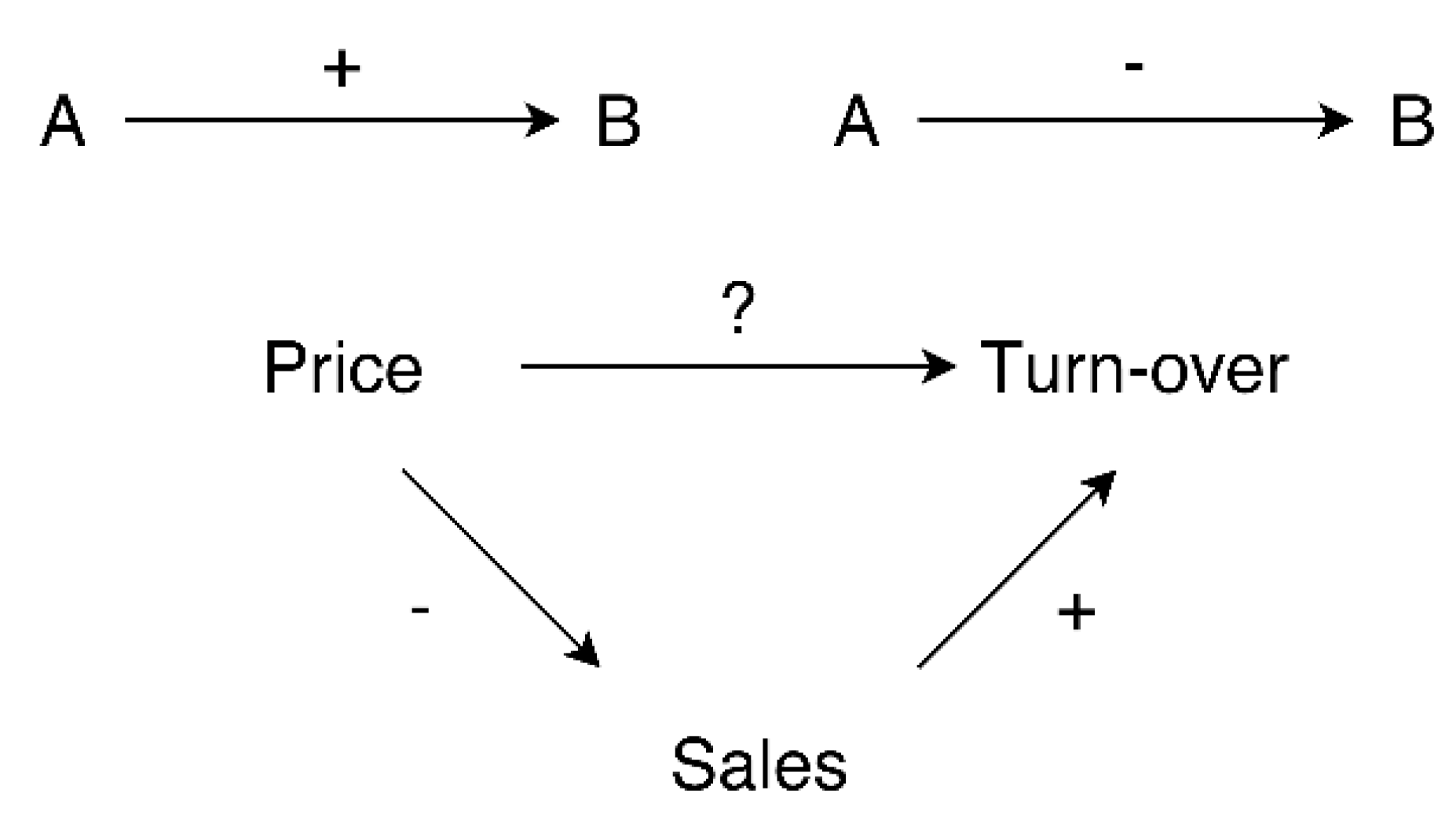
An important step preceding the formulation of the model itself is to determine the polarity between the elements, i.e., the positive and negative dependencies between the elements of the given system (Figure 2). It is sufficient to present this issue with examples taken from the field of Economics (Miller and Blair 2009). When there is a positive linkage between Elements A and B, for instnce the quantitative value augmentation of Element A that determines the value augmentation of Element B, then this relationship can be depicted with an orientational link from Element A to Element B with a plus sign. When there is a negative linkage, for instance the quantitative value augmentation of Element A determines the value decrease of Element B, then the sign is minus. This realtes to the relational analysis between two elements only (if this exists); however, it says nothing about the resulting behavior of the model; for example, the relationship between product price and final turn-over is not definite. As prices increase, sales decrease (a negative relationship), and as sales increase turnover increase as well (a positive relationship). Furthermore, cycles (reverse linkages) can occur in the diagram and the resulting polarity cannot be defined from the diagram (Santos 2006; Oliva et al. 2010).
Considering the facts presented above, it is possible to state that a basic definition of the single linkages and relationships in the elements of an individual system becomes a proficient starting point for the more complex dynamic modeling of failure impacts. Thus, the theoretical starting points of the dynamic modeling process will be formulated without direct linkages to the described facts.
The basic starting-point attributes of a dynamic system are the following: it is necessary to realize which physical quantities enter the model and their duration, the frequency of their observation which can be (for example, considering time) expressed in the form of continuous or discrete time. An element’s activity arises from mutual linkages, which determine the relationships between the observed quantities expressed in the form of a differential (Difference Equations), which define the system’s behavior. Ultimately, a dynamic system describes the behavior of the observed quantities, where their values are expressed in vector time x(t), expressed as the system state. The behavior of the observed system can then be expressed by the following equation (Equation (1)):
where, (t) = changes in the observed quantity in time; x(t) = descriptions of the actual state of the observed quantity; u(t) = conditions of control limitations; and t = the time dimension of the change of state.
The input u(t) can be perceived as being negative, i.e., as the disruption of a system’s functioning, as well as a positive device that keeps the system within the required operational regime. Naturally, the value of x(t), stated in time t, can be limited to a certain set X(t); that defines the acceptable system functionality boundaries. Therefore, they can thus be called “System Limitation Conditions” (Hromada et al. 2014). The nearer the value of the x(t) state quantity approaches the bounds of set X(t), the more critical is the state of the given system in time t, (in the CI disfunctionality state). Similarly, even the positive control u(t), is limited by a certain group of objective possibilities U(t) in time t, which can be classified as control limitation conditions. Apart from the above-mentioned conditions, conditions for optimality can also be taken into consideration (since they minimize costs, energies, time; and maximise profit, transport, etc.).
The role of optimum control in a time interval [t1, t2] can be formulated as follows: all controls u(t), which, in interval [t1, t2], conform to the control limitations u(t) ∈ U(t) conditions; and all results x(t) from equation (t) = f(x(t), u(t), t), which in the interval [t1, t2], conform to the conditions of state limitations x(t) ∈ X(t); and initial (in time t1) and final (in time t2) conditions x(t1) = a, x(t2) ∈ X(t2); then it is necessary to find the control u(t) value that conforms to the optimum condition. This is called the optimum control and the result obtained are the x(t), the optimum control response.
At the given moment t, the state x(t) changes in general and the level of change is its derivation (t); which is defined separately by a system of differential equations for each state quantity xi(t) (Equation (2)):
where = is the change of i-like quantity in time (derivation); xi = is the description of the actual state of the i-like quantity; ui = the quantity of i-like control; and t = the time-dimension of a change in state.
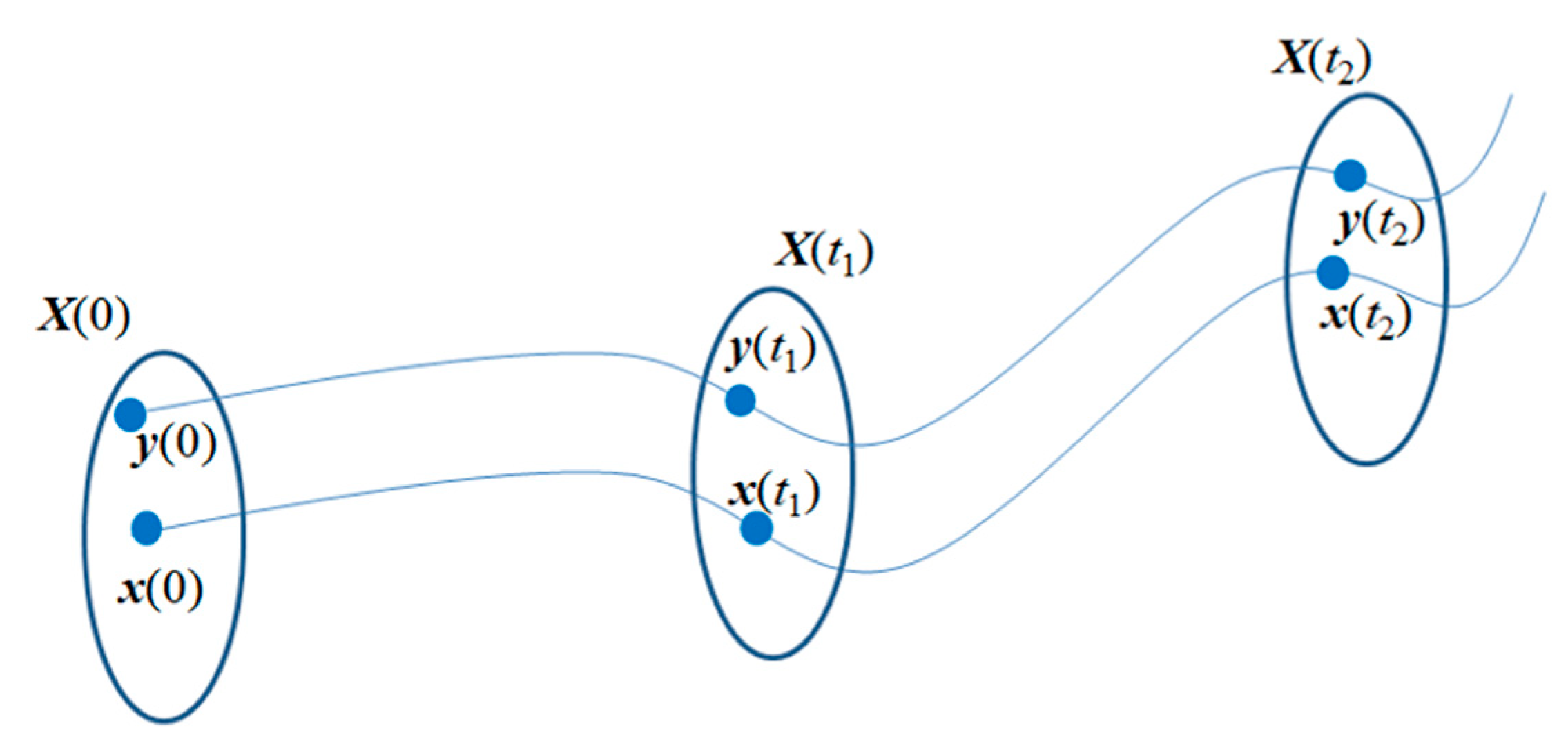
Let x(0) be the initial system state (i.e., the initial condition given, e.g., by the projection of the given CI). The solution of the optimum control issue is a vector x(t) = (x1(t), x2(t), …, xn(t)); its diagram is a curve (trajectory) in space Rn. With each different initial condition, one gets a different curve. The system of all trajectories forms the so-called phase portrait system, (Figure 3).
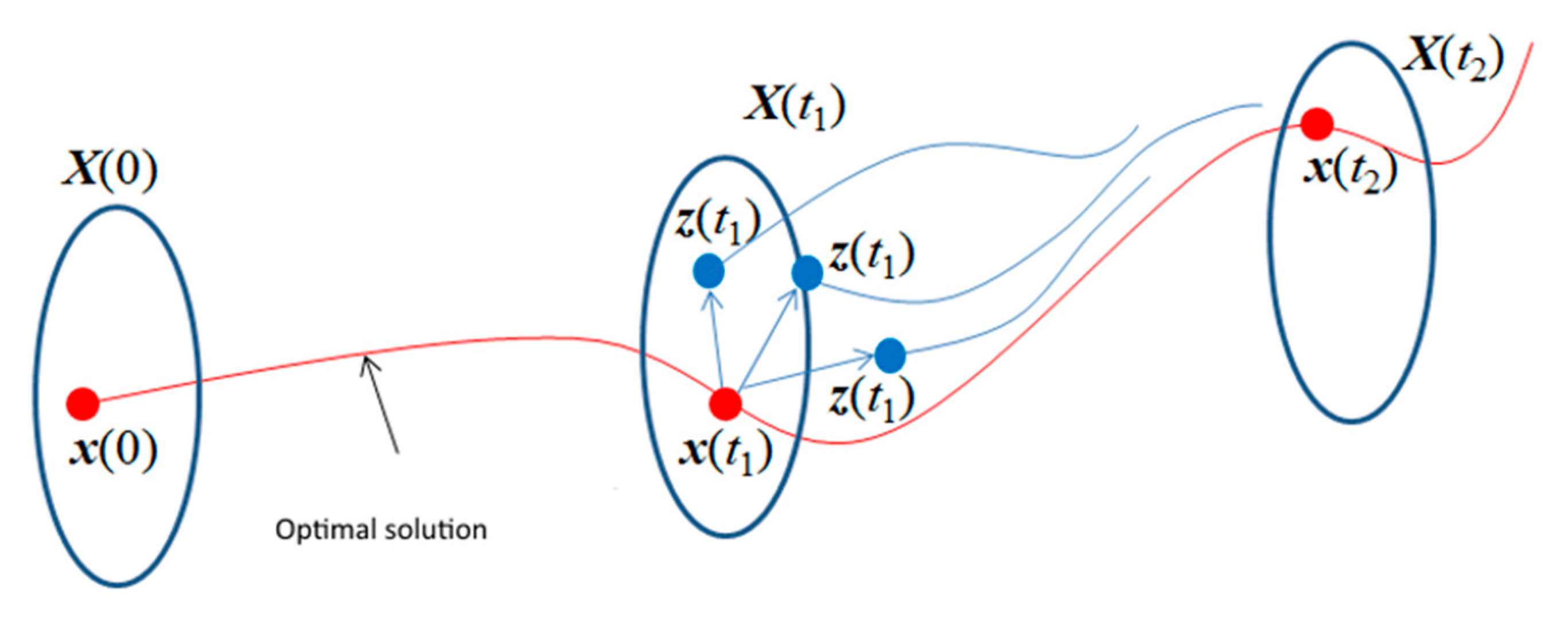
It can happen that in time t1, the system can be deflected from state x(t) to state z(t1) as a consequence of some kind of failure (Figure 4).
The state variable x(t) has been disrupted, and does not gain an optimum value in time t1. The nearer it approaches the state limitation line X(t1), the more disrupted the CI will be—in other words, it can be directly on the line or beyond it. Hence, the system’s trajectory will also be changed by t1. The presence of such a disruption causes changes to the initial conditions, for instance, the transition to a disrupted trajectory (cf. the blue lines in the Figures). The ovals in Figure 3 and Figure 4 represent constraints on the respective state values. The most interesting cases have been collated and formulated as a consequence of this process.
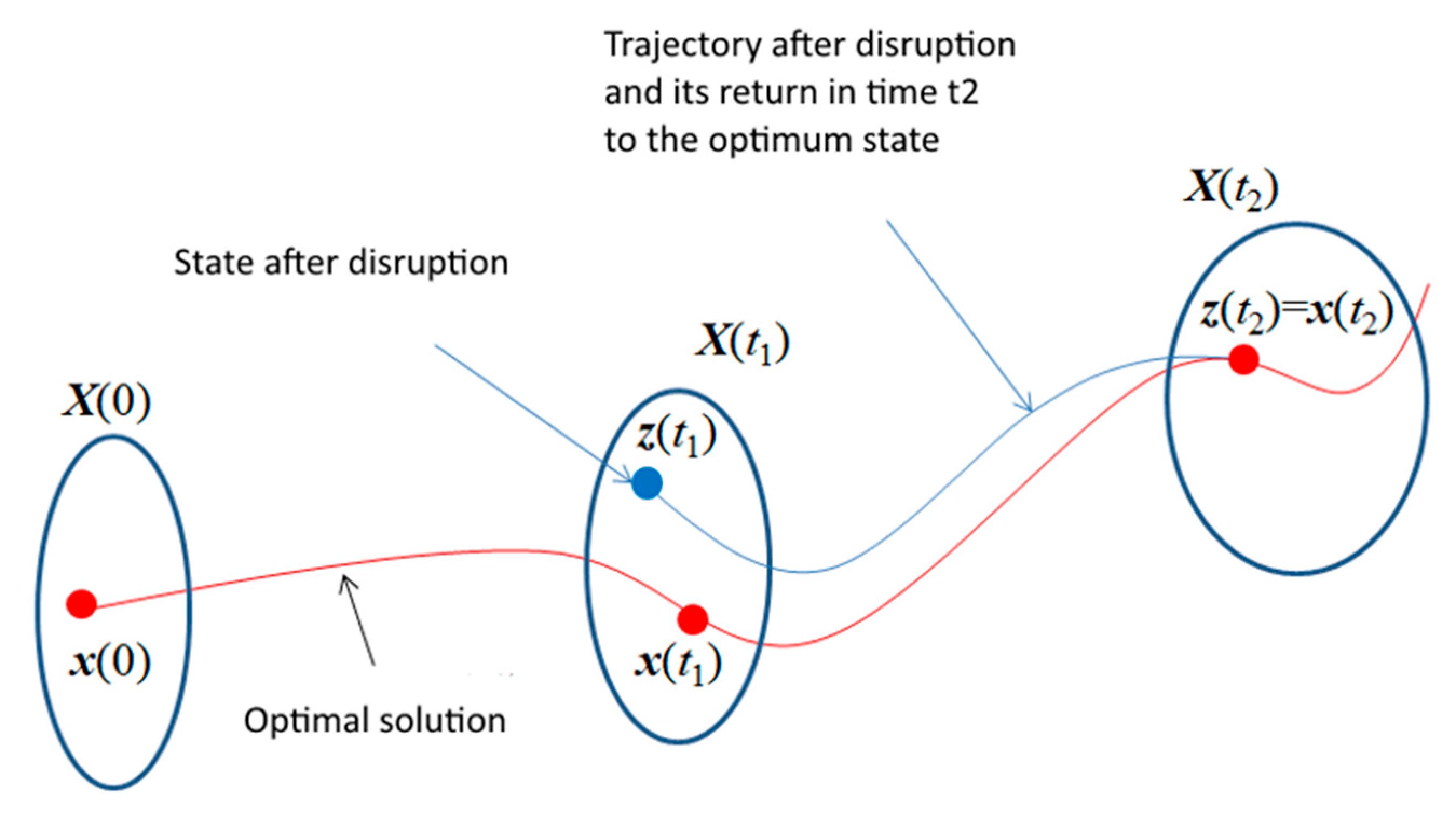
The system “deflects slightly” (disrupts) in time t1, and after some time, it attains the optimum state by itself; the ideal case adaptable systems (Figure 5).
The proficient framework enabled the formulation of theoretical solutions intended for further application on selected models and approaches relating to the issue of impact evaluation of the failure of objective Critical Infrastructure Systems.
These facts shall form the preliminary variables for the dynamic evaluation process of critical infrastructure correlative systems’ resistibility; as part of the RESILIENCE Project (2015). In conclusion, it is possible to state that the mathematical basis and approaches herein presented, shall form the starting-point for the formulation of a dynamic modeling system of impacts on road transport networks, within the context of the confrontation of the facts with current road transport modeling approaches.
2.3. Macroscopic Models as a Starting-Point for the Dynamic Modeling of Failures in Road Network Critical Infrastructure Elements
Connected with the above-mentioned, transport models used in Road Transport networks can be sub-divided into microscopic or macroscopic groups. Microscopic models are oriented on the mutual interaction of drivers, in the context of a complex system as a whole in which a significant role is played by their dynamic characteristics (Apeltauer et al. 2013). Macroscopic models are oriented on road networks’ global pararmeters and ignore the individual driver characteristics from the perspective of the problematical responses of a road network infrastructure as a whole, on the failure of its subsidiary elements, and are therefore, an optimal tool.
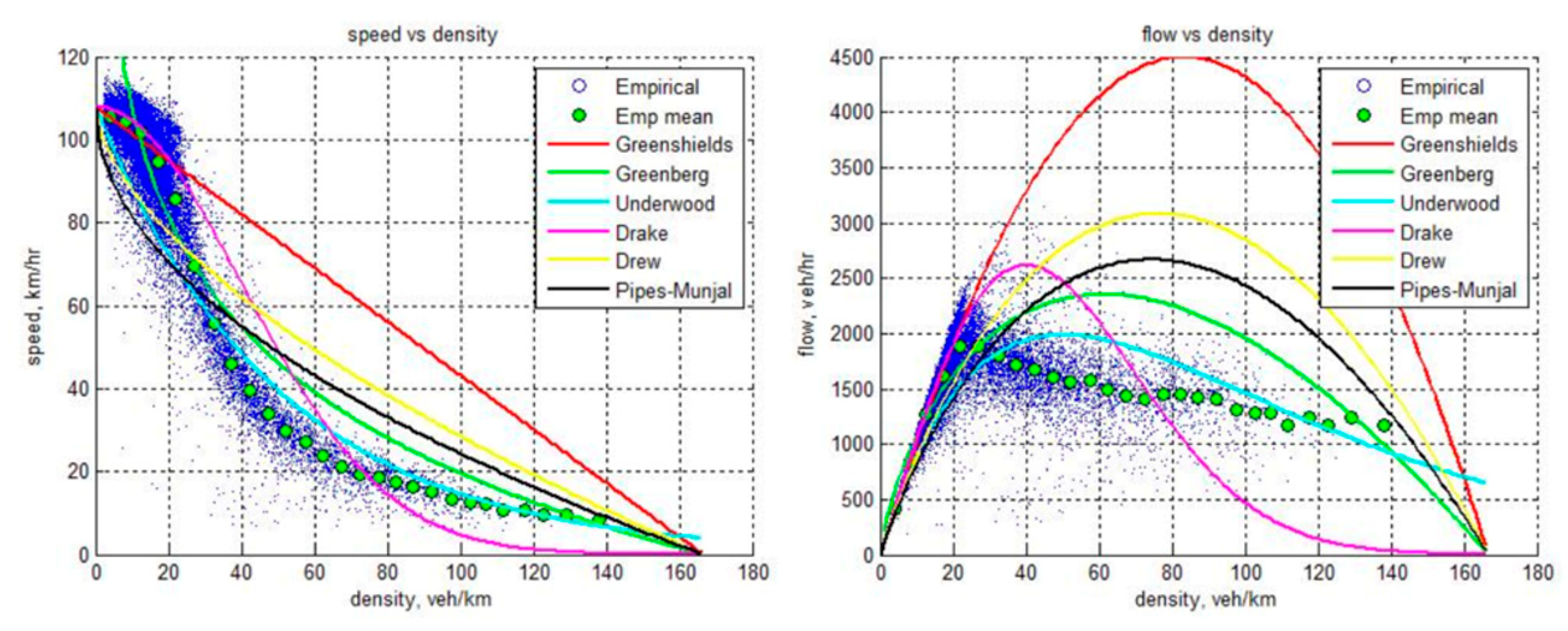
Macroscopic models are often used in road infrastructure impact modeling structures including Greenshild’s Linear Model, Greenberg’s Logarythmic Model, Underwood’s Exponential Model, and Pipe’s Generalised Model. Greenshild’s Model is one of the oldest and simplest macroscopic models, based on speed and intensity measurements that serve to calculate density (Bogo et al. 2015; Nakrachi and Popescu 2010). Concrete outcomes, using dynamic simulation modeling in road transport, are presented in the article “Increasing Transport Efficiency Using Simulation Modeling in a Dynamic Modeling Approach” (Upreti et al. 2014).
Macroscopic models are based on the relationship between the speed (v) … and density of the traffic stream (k); which assumes that, by increasing the density, i.e., the number of units of vehicles (pcs); so does speed decrease. Thus, its intensity can be defined with the help of Equation (3):
where, q = the intensity of traffic flow, [pcs∙h−1]; v = vehicle speed in the stream, and [km∙h−1]; k = vehicle density in the stream [pcs∙km−1].
The specific and direct relationships between these traffic flow status variables are the subject of long-term systematic research, and thus, cannot currently be described as universally valid (see Figure 6).
Greenshields’ Linear Model is the oldest and simplest, macroscopic model, based on the relationship between speed and intensity, which also allows one to calculate jam density (Bogo et al. 2015; Nakrachi and Popescu 2010). The main assumption being that speed and density are linearly related as can be seen in Equation (4):
where, vmax = maximum speed [km∙h−1]; kmax = congestion density [pcs∙km−1].
This model is unrealistic, mainly in the case of small densities, since vehicles do not influence one other in such a traffic state. Consequently, the linear relationship between speed and density is asymmetrical, i.e., the parabolic relationship of intensity on density. However, maximum intensity occurs through lower density. Further research has attempted to improve these invalidities, and many other models have been suggested. (Ni 2015; Chowdhury and Sadek 2003).
A key dynamic CIF impact modeling element is the selection of a relevant model, with regard to its scope and data detail. Macroscopic Models are much more suitable for the modeling of a vast affected region. A microscopic model would be better, should one only want to model a particular network, e.g., a crossroad, part of the transport overload; or a narrow gorge, while also considering congestion occurence and its transmittance. The choice of model is essential, mainly with regard to the input data, since macroscopic models require different data than microscopic models. Road transports modeling simulation tools, (Young et al. 2014) also play a significant role in this field.
One of the most crucial aspects of this process is task definition, in which it is necessary to focus on the safety management point-of-view. If this task concerns mobility planning in critical situations, it is possible to obtain data from various transport research studies and to use them as a base for the creation of element behavior in a given network. As an example, let us consider a road network model limited by the closure of a particularly important lane, where the model should reveal which of the surrounding roads will be used the most, and eventually, where the critical point that will be unable to divert a given traffic jam will occur. Such a model can be created thanks to several software tools or mathematical models, while the question of time and detail depends on the input data and output requirements.
However, if the model’s aim is to determine the progress of a future transport problem based on an infrastructure element failure, it is necessary to have access to real data, which can be very problematical. Currently, some of the potential tools that are able to work with real data are software tools like Aimsun Online from TSS-Transport Simulation Systems, S. L. Company, and the VISION Online production line from the PTV Group company.
These tools are capable of continuously processing real data from the terrain, furthermore, they can predict traffic streams that are dependent on the chosen model strategy in a network. By using such a model, it is possible to influence a transport network retroactively, e.g., by predicting travel time, dynamic instructions of integrated rescue system vehicles, predicting emissions, controlling overflow in cities, and affecting evacuation processes dynamically.
3. Proposal of a Dynamic Modeling System of Road Transport Impacts
Current macroscopic and microscopic models used in transport modeling are based on the assessment of vehicle movements and their interaction in traffic flows. Even though these approaches are modern, they do not regard the dynamic nature of degradation impacts modeling on operational parameters (i.e., road capacity) in a critical transport infrastructure. Considering these facts, the authors have developed a dynamic modeling system of impacts in road transport. The principle of this system is a stochastic approach, due to fact that the infrastructure elements’ failure and the extent of their impact, are based on probability estimation.
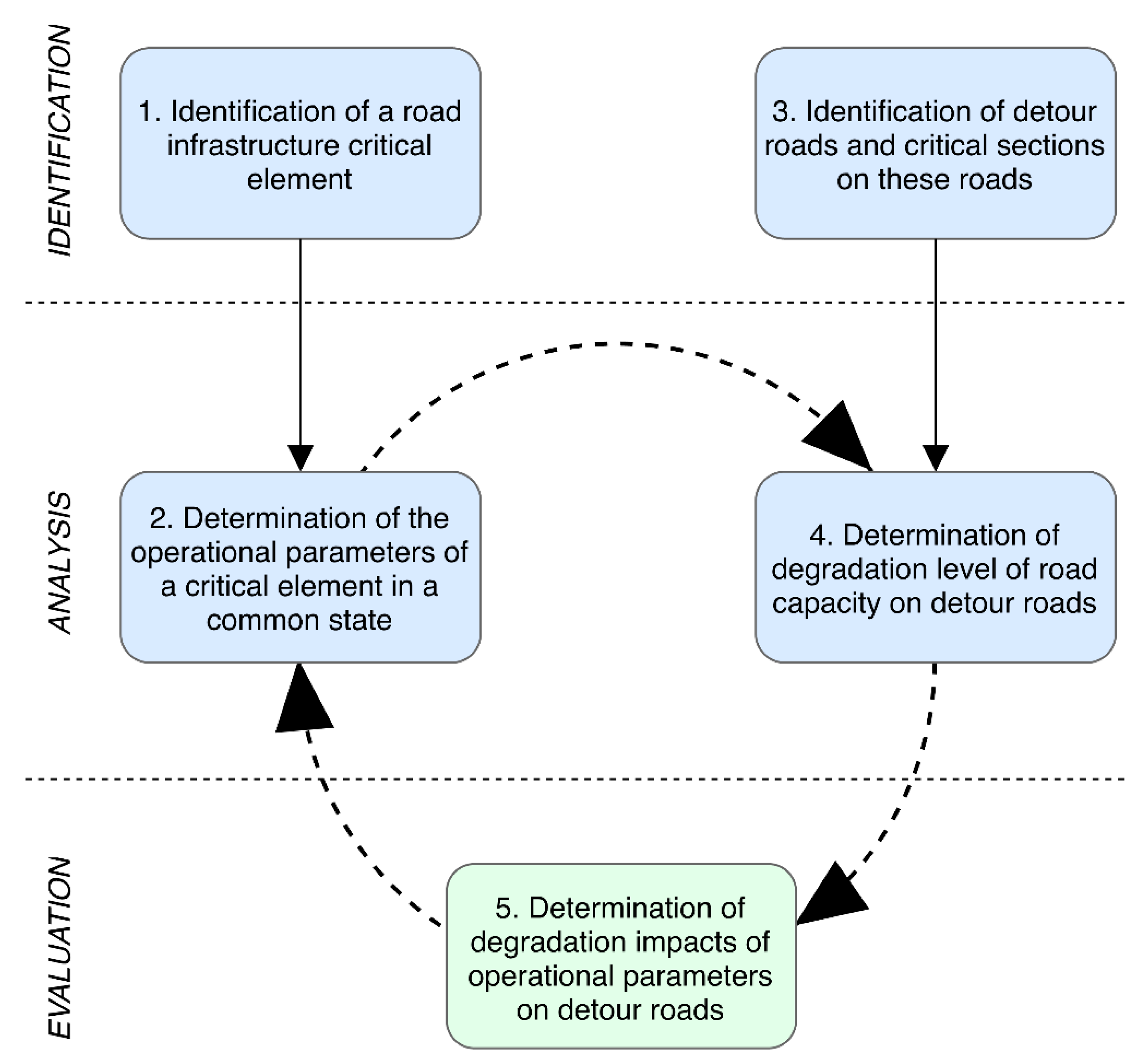
The comparative analysis of a road with a critical element and detour roads based on a macroscopic model is a fundamental element in this system. The system was developed for modeling the disruption or failure impact of European and national critical infrastructure elements (e.g., in the TEN-T framework); the use of microscopic models with regard to labor and computer technology limitations, is currently unrealistic. The core of this system is an algorithm (see Figure 7), which evaluates the operational parameters of these roads, the degradation level of road capacity, the capacity of detour roads, and the degradation impacts of the operational parameters on these detour roads.
Step 1: Identification of a Road Infrastructure Critical Element
Identification is a basic step in the dynamic modeling of impacts in the case of critical element elimination in a road network infrastructure. Based on the EU Directive (European Council 2008) and (Czech) national legal norms, these elements are identified and subsequently determined with regard to both sector and cross-cutting criteria; like for instance, European or national critical infrastructure elements. However, the fulfillment of such cross-cutting criteria (see Section 2.1, Critical Infrastructure Disruption or Failure Impacts), can only be assessed in conjunction with the impact modeling results, which are then compared with the values determined by the cross-cutting criteria. Therefore, the first necessity is the creation of an element criticality hypothesis, which is then subsequently either affirmed, or invalidated.
Step 2: Determination of the Operational Parameters of a Critical Element in a Common State
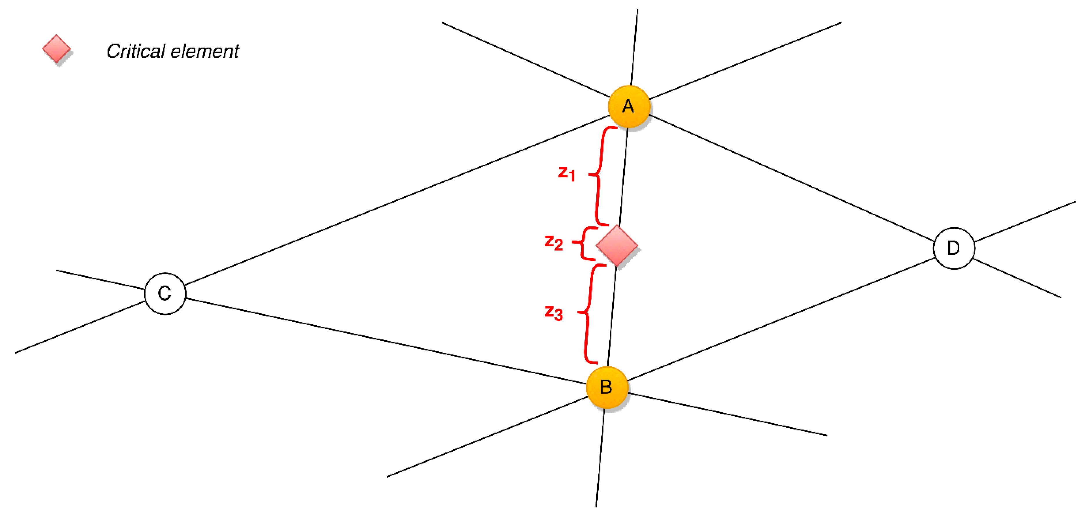
The second step of the algorithm requires one to determine the operational parameters of a critical element in a state, i.e., the road capacity level. Subsequently, these operational parameters need to be determined for the whole road on which this critical element is located. For a better demonstration of the system: this road located between Points A and B, will be designated as Road Z (see Figure 8).
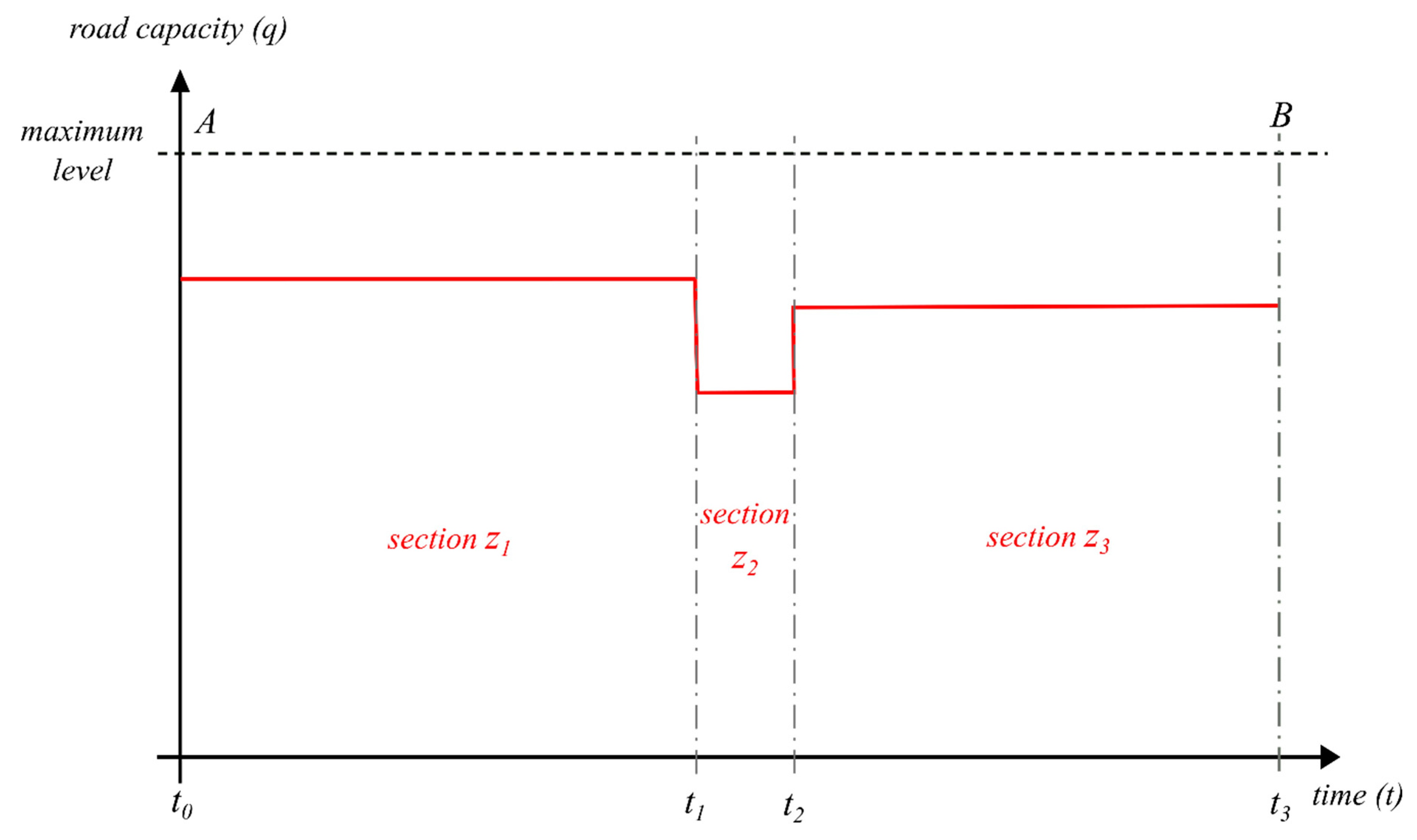
Road Z can be divided into three consecutive sections in road capacity terms. Sections z1 and z3 represent sections with a capacity corresponding to the type of road. The z2 section represents a critical element, i.e., a specific traffic section with reduced capacity, for example a narrowed section or a speed-restriction section. The development of the road capacity in these sections is plotted by considering constant functions in relation to time (see Figure 9).
Based on the findings from previous sections of this article and especially on the dynamic modeling of impacts in critical infrastructure (Canzani 2016), it is then possible to determine the total road capacity on the Road Z as the integral of the time function of the partial sections (Equation (5)):
where, qz = road capacity on Road Z [pcs∙h−1]; f(t) = road capacity function in time [pcs∙h−1]; c = road capacity constant [pcs∙h−1].
Step 3: Identification of Detour Roads and Critical Sections on These Roads
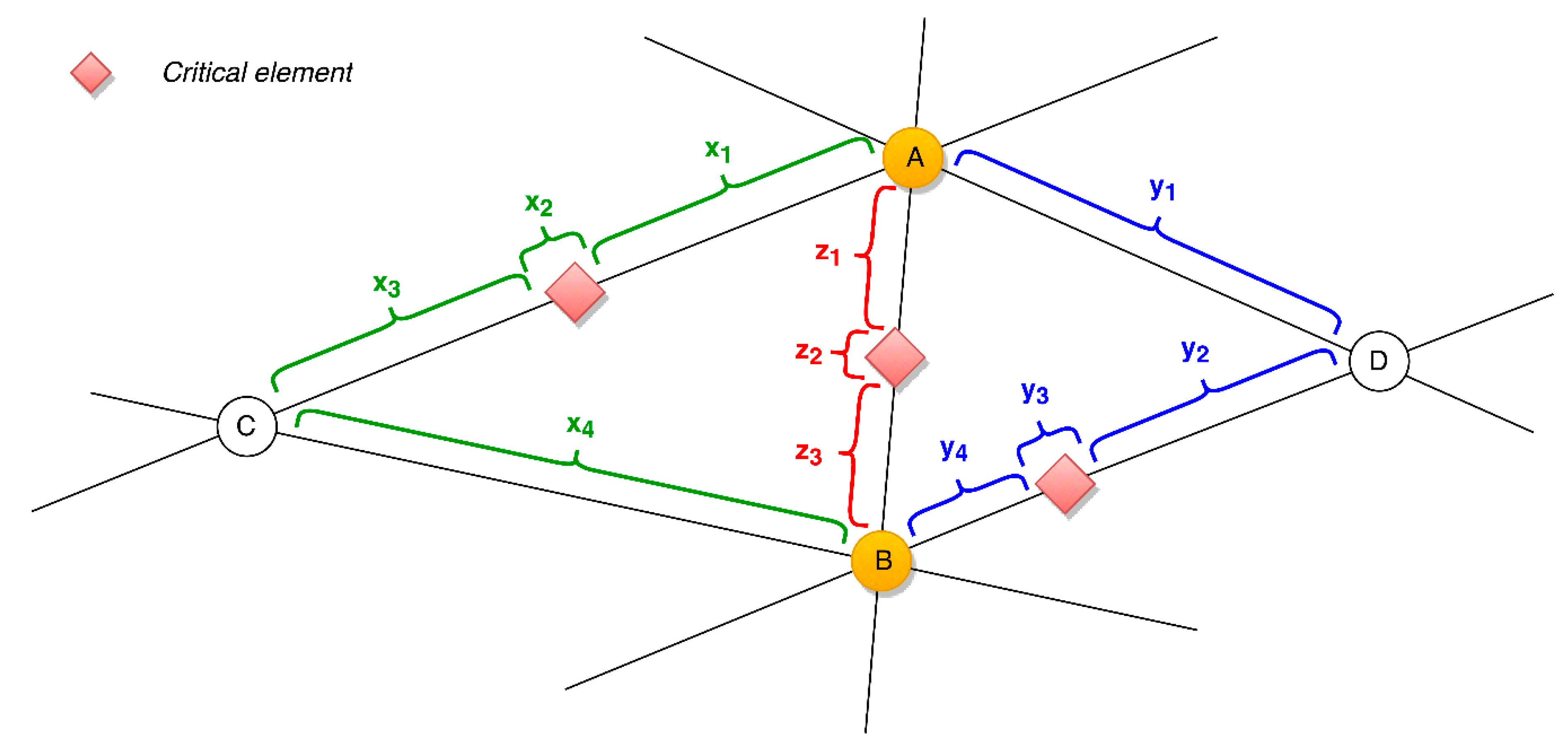
In the case of critical point disfunctions, it is necessary to search for detour roads and all of the critical sections located on them. For better clarification purposes, two sample detour roads were selected, i.e., Road X passing through Point C, and Road Y passing through Point D. Then, it is crucial to identify the critical sections. In the case of Road X, there is a section narrowed from two lanes to one lane. In the case of Road Y, there is a tunnel, which is momentarily undergoing reconstruction, and as a result, the speed limit has been lowered to 50 km∙h−1.
Step 4: Determining the Degradation Level of Road Capacity on Detour Roads
Just as for the original Road Z, in this case, the operational parameters of all of the critical elements of the detour roads need to be determined, i.e., the road capacity. Then, these operational parameters need to be determined for the entire Roads X and Y (see Figure 10).
In this case, both roads consist of four sections with varying road capacity, e.g., for Road X, these are sections x1, …, x4; where x1, x3 and x4 represent sections of capacity that correspond to the given type of road, and x2 is a critical element with reduced capacity, i.e., a section with a road that narrows from two lanes down to one lane. The calculation of the road capacity on the X and Y trajectories is performed analogously to Road Z according to the Equation (5).
Step 5: Determining Degradation Impacts of the Operational Parameters on the Detour Roads
The key step of the whole algorithm is to determine the degradation impacts of the operational parameters on the detour roads. The operational parameter degradation impacts can be expressed by the number of people affected and the economic losses expressed by the subsequent operational costs and lost GDP. Taking this into consideration, one must determine the length of the original and detour roads and the time needed to drive through them.
The road length can easily be obtained from maps; however, the time needs to be defined in relation to the density and capacity of the given roads. Therefore, it suffices to use Equation (3) for the calculation of the capacity and by its alteration, to obtain information about the time needed to travel through the given roads (Equation (6)):
where, q = road capacity [pcs∙h−1]; v = vehicle speed in flow [km∙h−1]; k = vehicle density in flow [pcs∙km−1]; s = length of the evaluated road [km]; t = time needed to drive through given road [h].
Afterwards, the economic losses due to operational costs caused by taking detour Road X as a consequence of the dysfunctionality of Road Z can then be calculated (Equation (7)):
where, EOC(X) = economic losses due to operational costs caused by taking detour Road X as a consequence of the dysfunctionality of Road Z [€∙h−1]; sx = detour Road X length [km]; sz = original Road Z length [km]; qz = road capacity on Road Z [pcs∙h−1]; eOC = operational costs [€∙km−1].
The economic losses to GDP caused by taking detour Road X as a consequence of the dysfunctionality of Road Z can be calculated by using Equation (8):
where, EGDP(X) = the economic losses to GDP caused by taking detour Road X as a consequence of the dysfunctionality of Road Z [€∙h−1]; tx = the time needed to drive through Road X [h]; tz = the time needed to drive through the original Road Z [h]; p = the number of people being transported [pcs∙h−1]; eGDP = GDP per capita [€∙pcs−1].
The resulting numbers of affected people p and economic losses (EOC + EGDP) must be averaged at a minimum for at least 24 h afterwards so that these can be compared with the numbers determined by the cross-cutting criteria (RAIN Project 2015). Dynamic impact character is actually dependent on road capacity—which is linked with traffic density—and the current state in a given section, which allows for the movement of vehicles at a certain speed. For example, in peak traffic hours, traffic density is much higher, which makes road capacity increase as well. An example of actual traffic density reports relating to the profile of the busiest Czech highway D1 over the past 24 h, can be found on the web portal (Traffic Density 2009).
4. Discussion
From the crisis management and critical infrastructure protection points-of-view, the dynamic modeling using macroscopic models results are important for the security of lives. The possibilities implied by cascading or synergistic impacts on road infrastructure are crucial to the functioning of the society as a whole. Further research must be aimed at detecting the interdependencies of individual subsectors and their mutual positive or negative influences. The continuous development of Information and Communication Technologies brings with it greater dependency of man on modern technologies, while also creating greater societal vulnerability. Intelligent transport systems have been in place in road transport matters for more than 10 years, and this dependence on information and communication technologies will continue to increase in line with the advent of electronic and autonomous vehicles. The challenge facing researchers is to optimise efficient automated road transport management resources within the context of the smart and safe city concept.
5. Conclusions
Road transport is a significant sub-sector of any national critical infrastructure and its disruption or failure can have serious impacts on other dependent sectors and their elements. Consequently, a synergistic effect can be formed that enhances the resulting negative impact on a society. Therefore, it is crucial for a transport critical infrastructure to have the requisite tools at its disposal allowing one to determine prompt and adequate reactions to potential emergency situations. One of the appropriate approaches—applicable in relation to the facts above—may be a Road Transport Impact dynamic modeling system, like the one presented above. The system was created using existing model simulation in transport tools, and their use thus offers a platform for the dynamic modeling of impacts, and this especially in the cross-cutting criteria field.
This contribution is also conceived from the perspective of the security research project: “RESILIENCE 2015: A Dynamic Resilience Evaluation of Inter-related Critical Infrastructure Subsystems”, where the facts are determined by enabling a dynamic critical infrastructure resilience evaluation within a defined territory whose outcome will determine the impact. Another benefit will be an objective selection of preventive measures to minimize risks to selected critical infrastructure subsectors in the safety, security, and crisis preparedness fields. Based on dynamic modeling and an assessment of a given critical infrastructure by means of this model, the process will subsequently be modified so as to be able to determine a list of road and rail transport critical infrastructures. This model, inter alia, also allows the modeling of failures of individual elements and the impact of these failures on the surrounding elements, as well as to design surveillance and technical security measures. These outputs will then be used as a basis for road transport infrastructure element determination and for the development of a modeling methodology and the development of a software tool for testing the performance of critical infrastructure elements in the transport sector.
In conclusion, it can be stated that dynamic impact modeling is suitable not only for the analysis of impacts that spread in time across sectors, but above all, as a support tool in road transport management. Dynamic modeling results serve as input information in order to be able to effectively minimize potential risks.
Author Contributions
Conceptualization, D.R.; Methodology, D.R., M.H. and M.R.; Validation, D.R., M.H., M.R. and Z.D.; Investigation, D.R. and M.R.; Writing—original draft preparation, D.R., M.H., M.R. and Z.D.; Visualization, D.R.; Supervision, D.R.; Project administration, D.R. and M.R.; Funding acquisition, D.R. and M.R.
Funding
This research was funded by the Ministry of the Interior of the Czech Republic, grant number VI20152019049 ‘Dynamic Resilience Evaluation of Interrelated Critical Infrastructure Subsystems’, the Technology Agency of the Czech Republic, grant number TE01020168 ‘Centre for Effective and Sustainable Transport Infrastructure’ and the VSB—Technical University of Ostrava, grant number SP2019/96 ‘Research of indicators of the occurrence of undesirable events disrupting the functional parameters of the components of the electricity-critical critical infrastructure’.
Acknowledgments
The authors are grateful to the reviewers for useful feedback that significantly improved the presentation.
Conflicts of Interest
The authors declare no conflict of interest.
References
- Alcaraz, Cristina, and Sherali Zeadally. 2015. Critical infrastructure protection: Requirements and challenges for the 21st century. International Journal of Critical Infrastructure Protection 8: 53–66. [Google Scholar] [CrossRef]
- Apeltauer, Tomas, Petr Holcner, Jiri Macur, and Michal Radimsky. 2013. Validation of microscopic traffic models based on GPS precise measurement of the vehicle dynamics. Promet Traffic & Transportation 25: 157–67. [Google Scholar]
- Attal, Stephane. 2010. Markov Chains and Dynamical Systems: The Open System Point of View. Ithaca: Cornell University. [Google Scholar]
- Bogo, Rudinei Luiz, Liliana Madalena Gramani, and Eloy Kaviski. 2015. Modeling the flow of vehicles by the macroscopic theory. Revista Brasileira de Ensino de Física 37: 1–8. [Google Scholar] [CrossRef]
- Brunovsky, Pavol. 1980. Mathematical Theory of Optimal Management. Bratislava: ALFA. (In Czech) [Google Scholar]
- Canzani, Elisa. 2016. Modeling Dynamics of Disruptive Events for Impact Analysis in Networked Critical Infrastructures. Paper presented at 13th Annual Conference for Information Systems for Crisis Response and Management (ISCRAM 2016), Rio de Janeiro, Brazil, May 22–25. [Google Scholar]
- Chowdhury, Mashrur A., and Adel Wadid Sadek. 2003. Fundamentals of Intelligent Transportation Systems Planning. Boston: Artech House. [Google Scholar]
- Dvorak, Zdenek, Jan Razdik, Radovan Sousek, and Eva Sventekova. 2010. Multi-agent system for decreasing of risk in road transport. Paper presented at 14th International Conference Transport Means, Kaunas, Lithuania, October 21–22. [Google Scholar]
- Dvorak, Zdenek, Bohus Leitner, and Ladislav Novak. 2013. The theoretical background for research of road transport elements vulnerability in Slovakia. Paper presented at 8th International Conference TRANSBALTICA, Vilnius, Lithuania, May 9–10. [Google Scholar]
- Dvorak, Zdenek, Eva Sventekova, David Rehak, and Zoran Cekerevac. 2017. Assessmnet oif Critical Infrastructure Elements in Transport. Procedia Engineering 187: 548–55. [Google Scholar] [CrossRef]
- European Council. 2008. Council Directive 2008/114/EC of 8 December 2008 on the Identification and Designation of European Critical Infrastructures and the Assessment of the Need to Improve Their Protection. Brussels: Council of the European Union. [Google Scholar]
- Government of the Czech Republic. 2010. Government Decree 432/2010 of 22 December 2010 on Criteria for Determination of the Critical Infrastructure Element; Prague: Government of the Czech Republic. (In Czech)
- Hromada, Martin. 2016. Cascade and Synergy Effect Modelling of Interrelated Critical Infrastructure Sub-Sectors. Habilitation Thesis, VSB—Technical University of Ostrava, Ostrava, Czech Republic. [Google Scholar]
- Hromada, Martin, Frantisek Kovarik, Ludek Lukas, Rostislav Richter, and Jan Valouch. 2014. Critical Infrastructure Protection of the Czech Republic in the Energy Sector. Ostrava: The Association of Fire and Safety Engineering. (In Czech) [Google Scholar]
- Jasenovec, Jan, and Zdenek Dvorak. 2018. Quantitative Assessment of Critical Infrastructure Sectors. Zilina: University of Zilina. (In Slovak) [Google Scholar]
- Kadri, Farid, Babiga Birregah, and Eric Châtelet. 2014. The impact of natural disasters on critical infrastructures: A domino effect-based study. Journal of Homeland Security and Emergency Management 11: 217–41. [Google Scholar] [CrossRef]
- Lovecek, Tomas, Jozef Ristvej, and Ladislav Simak. 2010. Critical Infrastructure Protection Systems Effectiveness Evaluation. Journal of Homeland Security and Emergency Management 7: 34. [Google Scholar] [CrossRef]
- Miller, Ronald E., and Peter D. Blair. 2009. Input-Output Analysis: Foundations and Extensions. Cambridge: Cambridge University Press. [Google Scholar]
- Nakrachi, Aziz, and Dumitru Popescu. 2010. Modelling and simulation of macroscopic traffic flow: A case study. Paper presented at 18th Annual International Mediterranean Conference on Control and Automation, Marrakech, Marocco, June 23–26. [Google Scholar]
- Ni, Daiheng. 2015. Traffic Flow Theory: Characteristics, Experimental Methods, and Numerical Techniques. Oxford: Elsevier. [Google Scholar]
- Oliva, Gabriele, Stefano Panzieri, and Roberto Setola. 2010. Agent-based input–output interdependency model. International Journal of Critical Infrastructure Protection 3: 79–82. [Google Scholar] [CrossRef]
- Ouyang, Min. 2014. Review on modeling and simulation of interdependent critical infrastructure systems. Reliability Engineering & System Safety 121: 43–60. [Google Scholar] [CrossRef]
- Ouyang, Min, Leonardo Dueñas-Osorio, and Xing Min. 2012. A tree-stage resilience analysis framework for urban infrastructure systems. Structural Safety 36: 23–31. [Google Scholar] [CrossRef]
- RAIN Project. 2015. Available online: http://rain-project.eu/about/the-scope-of-the-project/#land-vulnerability (accessed on 25 September 2018).
- Rehak, David, Jiri Markuci, Martin Hromada, and Karla Barcova. 2016. Quantitative evaluation of the synergistic effects of failures in a critical infrastructure system. International Journal of Critical Infrastructure Protection 14: 3–17. [Google Scholar] [CrossRef]
- Rehak, David, Pavel Senovsky, Martin Hromada, Tomas Lovecek, and Petr Novotny. 2018. Cascading Impact Assessment in a Critical Infrastructure System. International Journal of Critical Infrastructure Protection 22: 125–38. [Google Scholar] [CrossRef]
- RESILIENCE Project. 2015. Available online: http://www.resilience2015.cz/index.php/en (accessed on 14 November 2018).
- Rinaldi, Steven M., James P. Peerenboom, and Terrence K. Kelly. 2001. Identifying, understanding and analyzing critical infrastructure interdependencies. IEEE Control Systems Magazine 21: 11–25. [Google Scholar] [CrossRef]
- Santos, Joost R. 2006. Inoperability input-output modeling of disruptions to interdependent economic systems. Systems Engineering 9: 20–34. [Google Scholar] [CrossRef]
- Simak, Ladislav, and Jozef Ristvej. 2009. The Present Status of Creating the Security System of the Slovak Republic after Entering the European Union. Journal of Homeland Security and Emergency Management 6: 20. [Google Scholar] [CrossRef]
- Sventekova, Eva, Maria Luskova, and Zdenek Dvorak. 2016. Use of Network Analysis in Conditions of Critical Infrastructure Risk Management. Paper presented at 20th World Multi-Conference on Systemics, Cybernetics and Informatics (WMSCI 2016), Orlando, Florida, July 5–8. [Google Scholar]
- Sventekova, Eva, Bohus Leitner, and Zdenek Dvorak. 2017. Transport critical infrastructure in Slovak republic. Paper presented at 8th International Multi-Conference on Complexity, Informatics and Cybernetics (IMCIC 2017), Orlando, Florida, March 21–24. [Google Scholar]
- Traffic Density. 2009. Traffic Density in the D1 Highway Profil. Available online: http://portal.dopravniinfo.cz/en/d1-motorway-traffic-density (accessed on 31 January 2019).
- Trucco, Paolo, Enrico Cagno, and Massimiliano De Ambroggi. 2012. Dynamic functional modelling of vulnerability and interoperability of critical infrastructures. Reliability Engineering & System Safety 105: 51–63. [Google Scholar] [CrossRef]
- Upreti, Girish, Prasanna V. Rao, Rapinder S. Sawhney, Isaac Atuahene, and Rajive Dhingra. 2014. Increasing transport efficiency using simulation modeling in a dynamic modeling approach. Journal of Cleaner Production (Special Volume: Making Progress Towards More Sustainable Societies through Lean and Green Initiatives) 85: 433–41. [Google Scholar] [CrossRef]
- Vidrikova, Dagmar, Zdenek Dvorak, and Veroslav Kaplan. 2011. The current state of protection of critical infrastructure elements of road transport in the conditions of the Slovak Republic. Paper presented at 15th International Conference Transport Means, Kaunas, Lithuania, October 20–21. [Google Scholar]
- Vidrikova, Dagmar, Kamil Boc, Zdenek Dvorak, and David Rehak. 2017. Critical Infrastructure and Integrated Protection. Ostrava: The Association of Fire and Safety Engineering. [Google Scholar]
- Young, William, Amir Sobhani, Michael G. Lenné, and Majid Sarvi. 2014. Simulation of safety: A review of the state of the art in road safety simulation modelling. Accident Analysis & Prevention 66: 89–103. [Google Scholar] [CrossRef]
- Zagorecki, Adam, Jozef Ristvej, and Krzysztof Klupa. 2015. Analytics for protecting critical infrastructure. Communications Scientific Letters of the University of Zilina 17: 111–15. [Google Scholar]
Figure 1.
Aspects that create the impact character in a critical infrastructure system (Rehak et al. 2016).
Figure 1.
Aspects that create the impact character in a critical infrastructure system (Rehak et al. 2016).

Figure 2.
Reverse linkages diagram (Miller and Blair 2009).
Figure 2.
Reverse linkages diagram (Miller and Blair 2009).

Figure 3.
Phase portrait system.

Figure 4.
System deflection.

Figure 5.
Adaptable systems.

Figure 6.
Basic diagrams comparing macroscopic traffic flow status model variables (Ni 2015).
Figure 6.
Basic diagrams comparing macroscopic traffic flow status model variables (Ni 2015).

Figure 7.
Algorithm of a road transport impact dynamic modeling system.

Figure 8.
Graphic depiction of a road with an identified critical element.

Figure 9.
Road capacity and time dependency.

Figure 10.
Graphic depiction of detour roads divided into given segments.

© 2019 by the authors. Licensee MDPI, Basel, Switzerland. This article is an open access article distributed under the terms and conditions of the Creative Commons Attribution (CC BY) license (http://creativecommons.org/licenses/by/4.0/).
Share and Cite
MDPI and ACS Style
Rehak, D.; Radimsky, M.; Hromada, M.; Dvorak, Z. Dynamic Impact Modeling as a Road Transport Crisis Management Support Tool. Adm. Sci. 2019, 9, 29. https://0-doi-org.brum.beds.ac.uk/10.3390/admsci9020029
AMA Style
Rehak D, Radimsky M, Hromada M, Dvorak Z. Dynamic Impact Modeling as a Road Transport Crisis Management Support Tool. Administrative Sciences. 2019; 9(2):29. https://0-doi-org.brum.beds.ac.uk/10.3390/admsci9020029
Chicago/Turabian StyleRehak, David, Michal Radimsky, Martin Hromada, and Zdenek Dvorak. 2019. "Dynamic Impact Modeling as a Road Transport Crisis Management Support Tool" Administrative Sciences 9, no. 2: 29. https://0-doi-org.brum.beds.ac.uk/10.3390/admsci9020029
Note that from the first issue of 2016, this journal uses article numbers instead of page numbers. See further details here.