The Application of Frequency-Temperature Superposition Principle for Back-Calculation of Falling Weight Deflectometer

1
Central Region Branch Office, Freeway Bureau, MOTC, New Taipei City 24303, Taiwan
2
Department of Civil Engineering, National Chung Hsing University, Taichung City 40227, Taiwan
*
Author to whom correspondence should be addressed.
Appl. Sci. 2020, 10(1), 132; https://0-doi-org.brum.beds.ac.uk/10.3390/app10010132
Submission received: 15 November 2019
/
Revised: 19 December 2019
/
Accepted: 20 December 2019
/
Published: 23 December 2019
Abstract
:The falling weight deflectometer (FWD) is a widely used nondestructive test (NDT) device in pavement infrastructure. A FWD test measures the surface deflections subjected to an applied impact loading and the modulus of pavement layers can be determined by back-calculating the measured deflections. However, the modulus of asphalt layers is significantly influenced by temperature; hence, the temperature correction must be considered in back-calculation to evaluate the moduli of asphalt layers at a reference temperature. In addition, the in situ temperature at various pavement depths is difficult to measure. A model for evaluating the temperature at various depths must be established to estimate the in situ temperature of asphalt layers. This study collected the temperature data from a FWD test site to establish a temperature-evaluation model for various depths. The cored specimens from the test site were obtained to conduct dynamic modulus tests for asphalt layers. The FWD tests were applied at the FWD test site and the back-calculation was performed with temperature correction using the frequency-temperature superposition principle. The back-calculated moduli of asphalt layers were compared with the master curve of dynamic modulus to verify the application of the frequency-temperature superposition principle for FWD back-calculation. The results show that the proposed temperature-evaluation model can effectively evaluate the temperature at various depths of pavement. Moreover, the frequency-temperature superposition principle can be effectively employed to conduct temperature correction for FWD back-calculation.
1. Introduction
The bearing capacity of pavement structure is determined by integrating the modulus of each pavement layer [1,2]. However, the bearing capacity of pavement structure decreases with increasing loading and amount of traffic, and it is not efficient to evaluate the in situ structural modulus of each pavement layer using in situ core drilling. Hence, development of nondestructive tests and back-calculation for detecting the structural modulus of pavement structures is critical and necessary.
A falling weight deflectometer (FWD) is a widely used nondestructive test in pavement engineering for evaluating the modulus of each pavement layer. A FWD measures the deflection on the pavement surface subjected to impact loading. Then, the modulus of the pavement layer can be obtained by back-calculation of the measured surface deflections [3,4,5,6]. The back-calculation analysis conducts iterations of structural analysis (e.g., finite element analysis and multi-layer theory) until the calculated surface deflection matches the measured deflection. Senseney [7] and Ahmed [8] conducted lightweight FWD tests and a dynamic finite element analysis model was used to analyze and verify experimental data and to determine the mechanical properties of a road foundation layer comprising a mixture of limestone and bottom slag from an incinerator. Varma et al. [9] simulated pavement with linear or nonlinear elasticity in a back-calculation to analyze the deflections for obtaining the material properties of various layers. Since asphalt material exhibits viscoelasticity with small deformations [10,11], Kutay et al. [11] employed Schapery viscoelastic theory and performed a back-calculation to determine the dynamic modulus master curve of asphalt pavement through the surface deflection obtained using an FWD. During the iteration process, multilayer-viscoelasticity theory was employed to identify the linear viscoelastic characteristics of asphalt pavement.
Since FWD deflection measurements are related to temperature for asphalt layers, scholars have proposed that the back-calculation of FWD deflection measurements should be temperature-corrected to a reference temperature and the temperature-correction should be dependent on the properties of the asphalt itself [12,13,14,15]. However, actual in situ temperature data of asphalt layers are difficult to obtain. Therefore, a temperature prediction model must first be established for temperature-correction. On the basis of the BELLS temperature prediction model proposed by Lukanen et al. [16], Park et al. [17] established a temperature prediction model appropriate for Michigan State in the United States by using temperature data from the seasonal monitoring of the US Long-Term Pavement Performance project. Park et al. [18] and Marshall et al. [19] verified another model, named BELLS3, in North Carolina and Tennessee, respectively. Zheng et al. [20] employed the BELLS equations as a basis for establishing a temperature prediction model for Henan, China.
In terms of temperature correction, the effect of temperature on the modulus of an asphalt layer has been assessed using a master curve or by conducting deflection value correction to ensure the consistency of evaluation standards. The dynamic moduli obtained using a material test system or through FWD back-calculation were employed to calculate temperature-correction factors, facilitating comparison between data obtained at the same temperature. The Mechanistic-Empirical Pavement Design Guide states that dynamic modulus tests should typically be used to evaluate the linear viscoelasticity of asphalt concrete and determine the effects of various asphalt materials on temperature and frequency [21,22,23]. When tests are conducted at different temperatures and load frequencies with the application of continuous sine waves, the relationship between stress and strain measurements can be expressed by the complex dynamic modulus (E*). Seo et al. [24] used the S-shaped function for the master curve to determine that the parameters in the function were influenced by the screening percentage, void fraction, and asphalt content, respectively. Subsequently, they estimated different frequencies by using the viscosity and obtained a new master curve equation appropriate for the use of in situ FWD results, specifically for analyzing in situ material conditions. Solatifar et al. [25] employed the Witczak model [26,27,28] to predict the master curve of the dynamic modulus. By using shift factors acquired in the laboratory, a master curve of FWD data was constructed to serve as the in situ dynamic modulus master curve, which could be used to determine the extent of material damage. In the Long-Term Pavement Performance project, Killingsworth [29] investigated the relationship between deflection, back-calculation results and pavement temperature. The Washington State Department of Transportation conducted regression analysis on the relationship between the dynamic modulus of traditional dense-graded asphalt mixtures and pavement temperature and proposed a temperature-correction coefficient for the back-calculated modulus of the asphalt mixture layer. Ye et al. [30] and Zhou et al. [31] used the exponential function to perform data fitting and adjusted the moduli to the reference temperature. Chen et al. [32] developed separate temperature-correction functions for deflections and moduli, determining that only deflections at test points close to the falling weight disk were significantly affected by temperature.
2. Research Objectives and Significance
Since the modulus of asphalt layer is significantly affected by temperature, the temperature correction must be conducted for the asphalt layer when conducting FWD back-calculation in order to evaluate the modulus of the asphalt layer at the same temperature. Moreover, measuring the temperatures at various road depths in situ is difficult, and a model must be established for estimating the temperature at various depths of asphalt layers. Hence, this study conducted the FWD tests and collected the temperature data at various depths in roads at the FWD test site constructed by Taiwan’s Freeway Bureau. The objectives of this study are:
- To establish a temperature-evaluation model for various pavement depths by performing the regression analysis of temperature measurements at various depths in the test site.
- To perform in situ core drilling in the test site and conduct the dynamic modulus test for obtaining the master curve and the relationship between temperature and frequency.
- To conduct FWD tests in the test site at different temperatures and to apply the temperature correction for FWD back-calculation.
- To verify the effectiveness of the frequency-temperature correction by comparing the master curve of the dynamic modulus obtained in the laboratory and the back-calculated modulus for asphalt layers.
3. FWD and Test Site
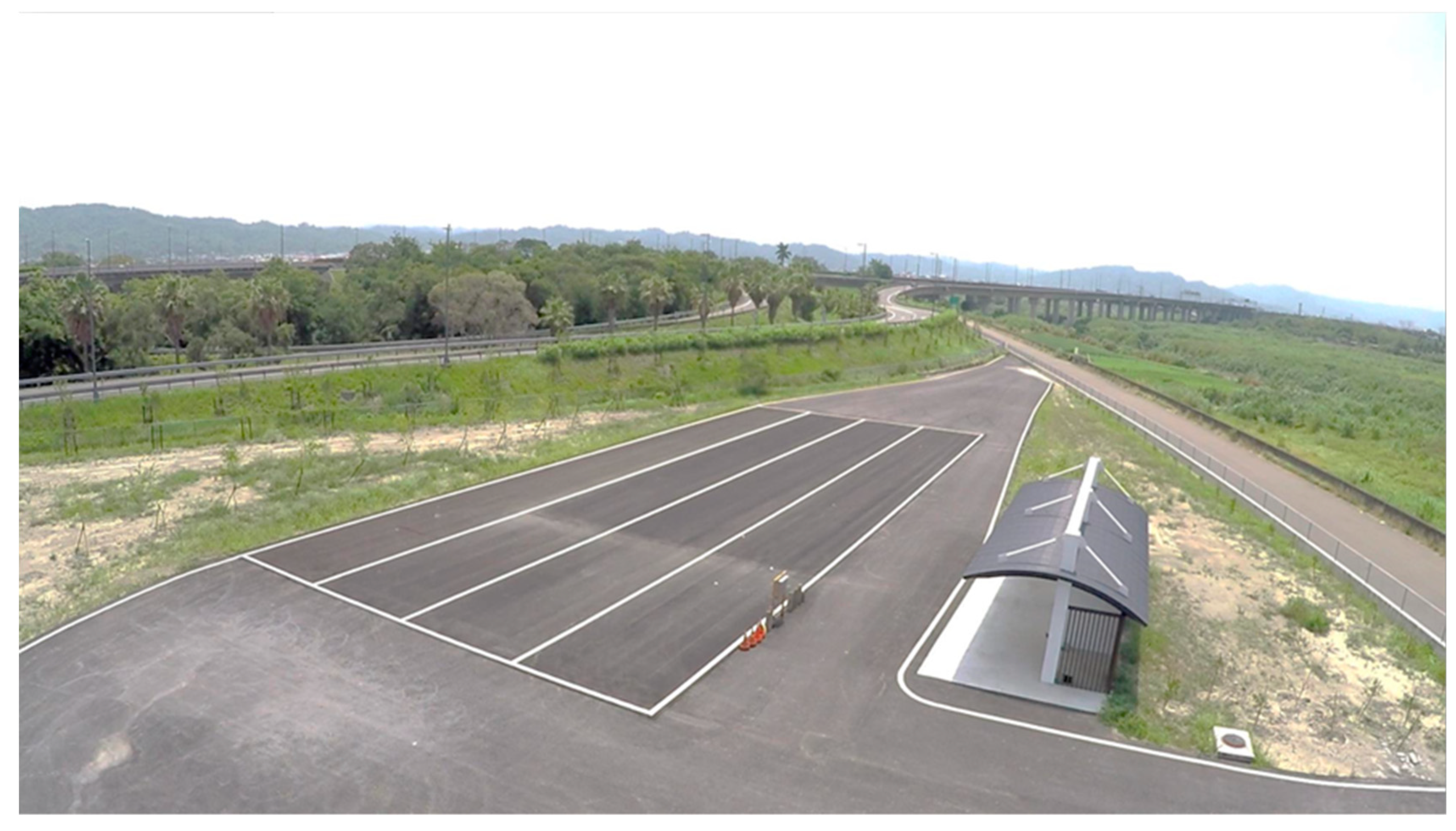
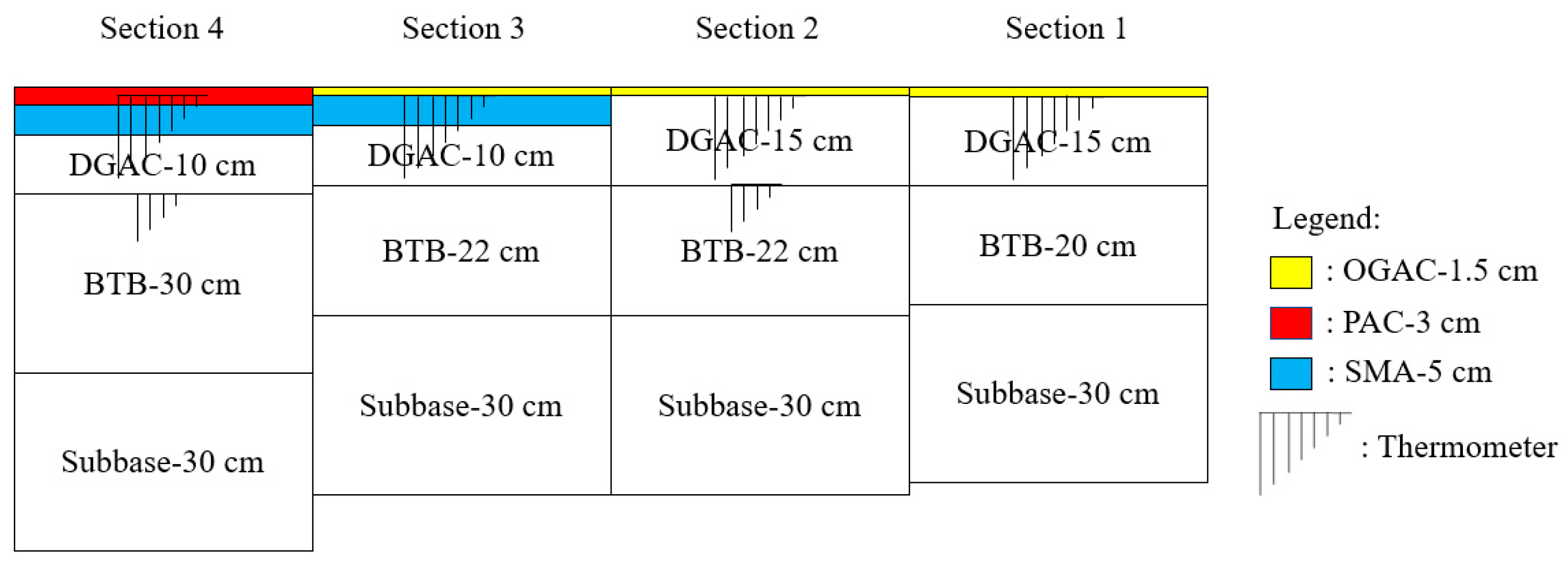
Figure 1 and Figure 2 are an aerial photograph and a top-view schematic of the FWD test site constructed by Taiwan Freeway Bureau, respectively. Four types of cross-section which are commonly used in Taiwan freeway pavement structures were constructed at the test site. The length of the test road is 50m, while the width of each pavement cross-section is 5 m. Figure 3 illustrates the schematic for each cross-section. For all cross-sections, an aggregate-type subbase with 30 cm thickness was constructed on a well-compacted subgrade. For cross-sections 2 and 3, a 22-cm-thick bitumen-treated base (BTB) was paved on the aggregate subbase, whereas the thicknesses of BTB layer were 20 cm and 30 cm on the aggregate subbase for cross-sections 1 and 4, respectively. A dense-graded asphalt concrete (DGAC) layer with 15 cm thickness above BTB and 1.5 cm thickness of open-graded asphalt concrete (OGAC) on DGAC layer were constructed for both cross-sections 1 and 2. In cross-sections 3 and 4, DGAC layer with 10 cm thickness and 5 cm thickness of stone mastic asphalt (SMA) were laid on the top of BTB layer. Then, 1.5 cm thickness of OGAC and 3-cm-thick porous asphalt concrete (PAC) were constructed above the SMA layer in sections 3 and 4, respectively. Table 1 details the asphalt binder type and the percentage of binder content for DGAC, OGAC, PAC, SMA, and BTB. The PAC and SMA were made from Type-III modified asphalt binder, whereas the binder types of remaining materials were AC-20.
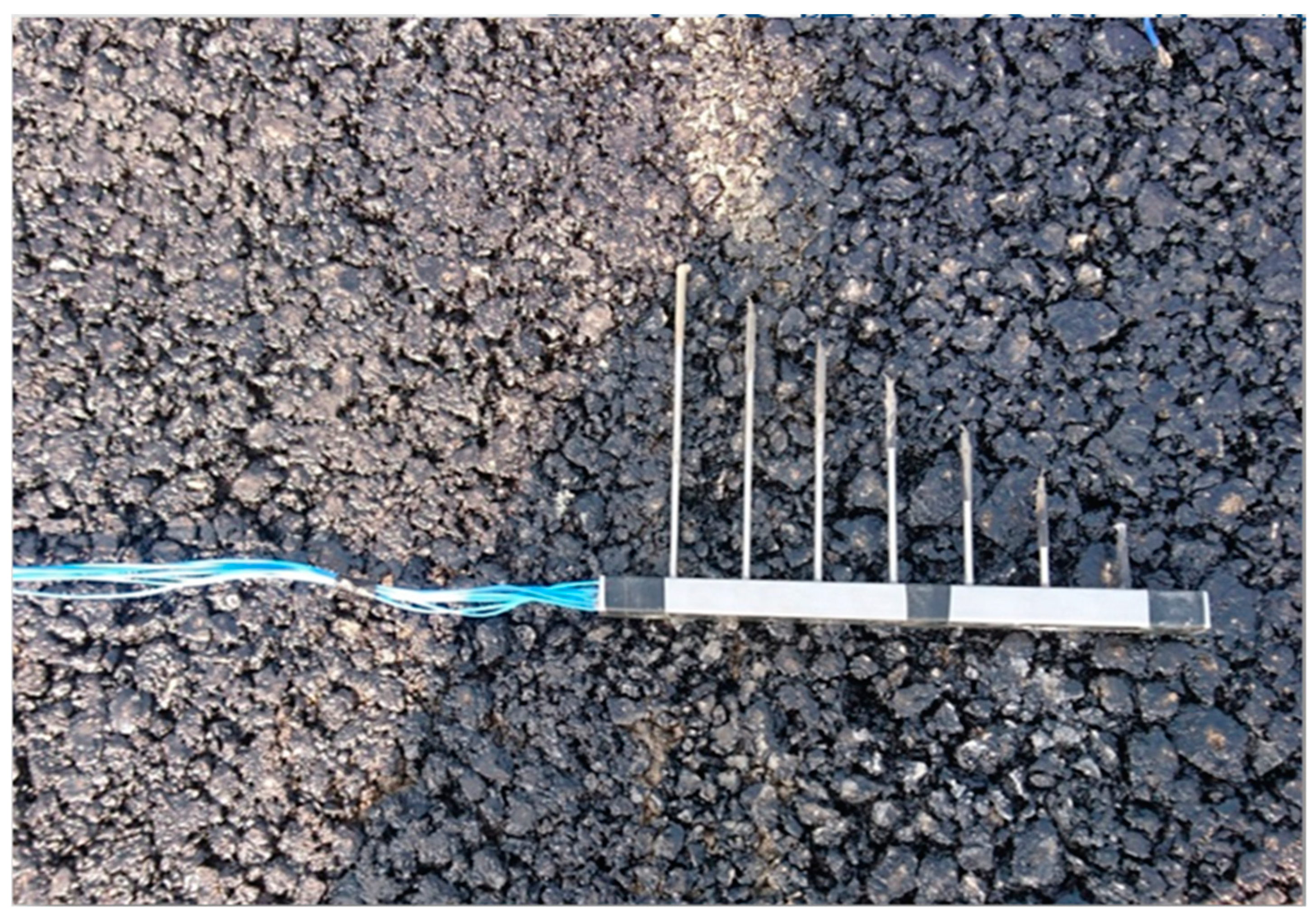
In order to develop the temperature-evaluation model and to conduct the temperature correction for FWD back-calculation, thermometers were installed in the FWD test site for the measurements of temperature. Figure 4 shows a photograph of the thermometers buried in the road section. The locations and depths of the buried thermometers are indicated in Figure 2 and Figure 3, respectively. The specific depths of thermometers were buried 3.5, 5.5, 7.5, 9.5, 11.5, 13.5, 15.5, 18.5, 20.5, 22.5, and 24.5 cm below road surface, 11 depths in total. The surface and atmospheric temperature at the test road were also recorded in the test site using a data miner at a frequency of one record per hour.
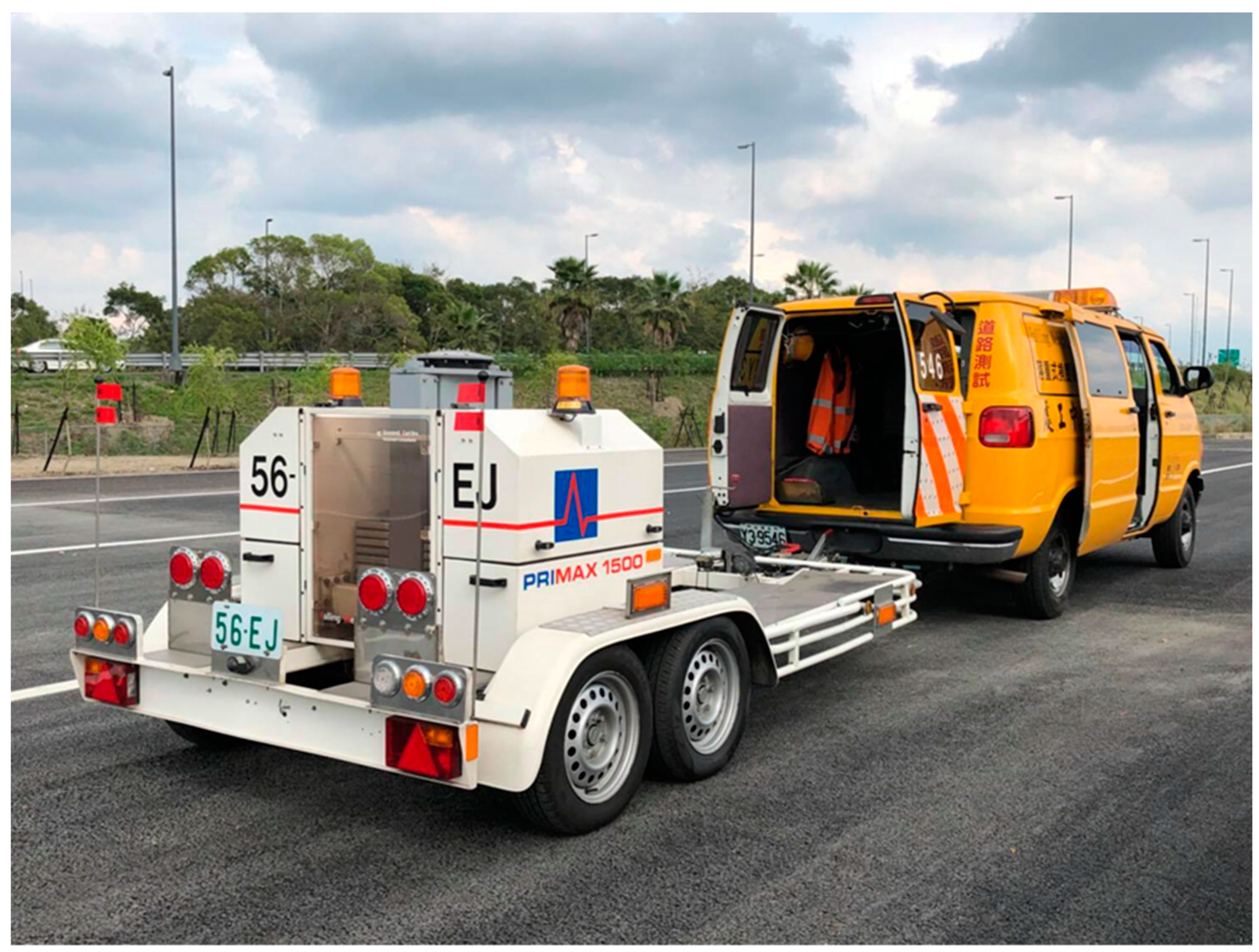
A PRIMAX 1500 FWD device as shown in Figure 5 was employed in this study. The FWD device applied an impact loading and the surface deflections were measured at 12 locations such as 0, 200, 300, 400, 500, 600, 700, 900, 1200, 1500, 1800, and 2100 mm away from the center of the falling-weight disk. Afterwards, the measured deflections can be entered into the back-calculation software to obtain the modulus of each pavement layer. This research conducted the FWD test at different temperatures (i.e., in the morning, at noon, and in the afternoon) to investigate the effect of temperature on the FWD test and back-calculation results.
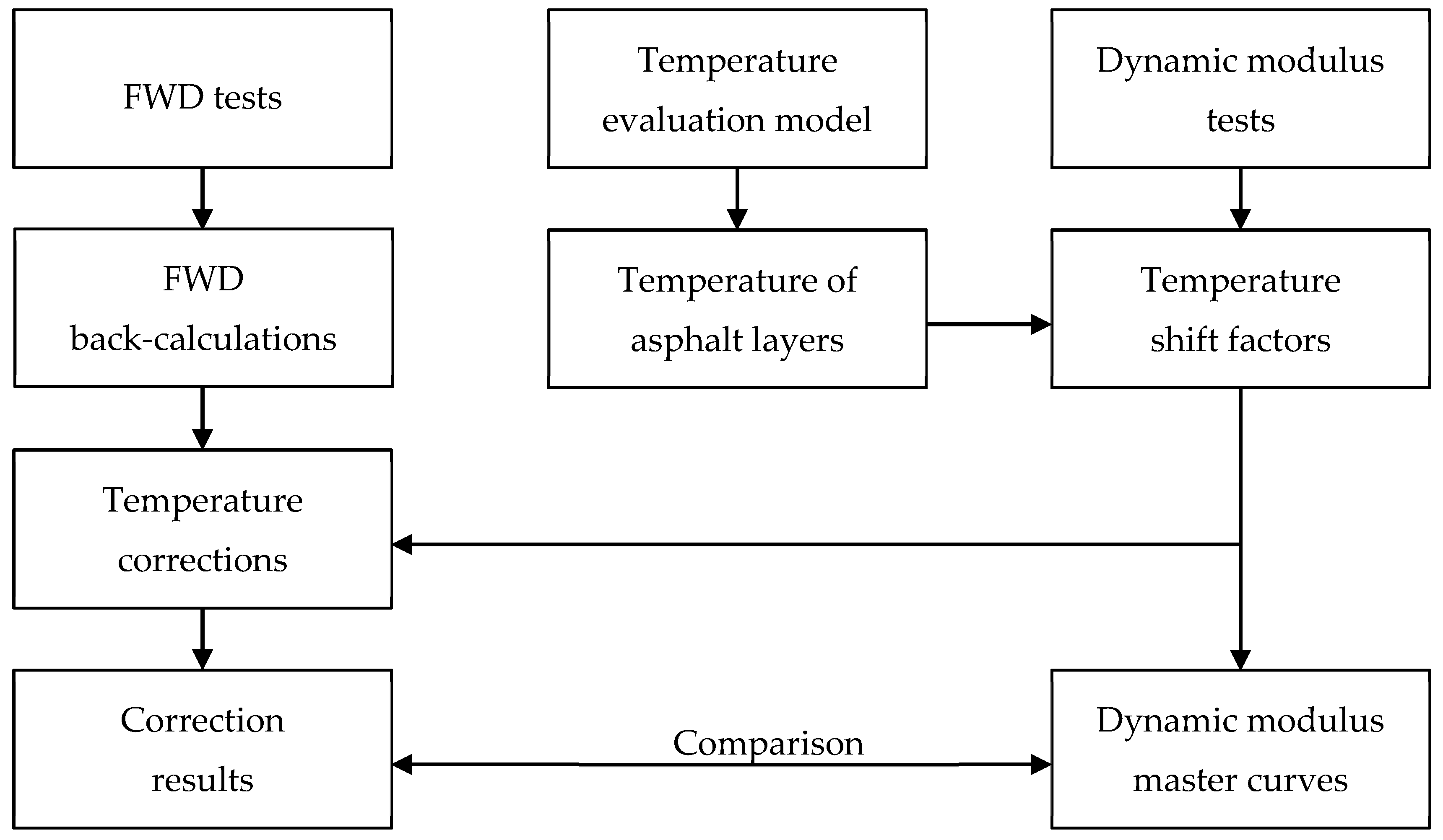
To determine the modulus and the relationship between temperature and frequency of the asphalt material layers such as the DENSE and BTB layers, this study performed in situ core drilling on the test roads. The drilled cores were then subject to dynamic modulus tests in a laboratory to obtain a master curve of the dynamic modulus and frequency-temperature shift factors. Subsequently, the frequency-temperature shift factors were used in FWD back-calculation to conduct the temperature correction. Through comparison of the shifted modulus and the dynamic modulus master curve, the effectiveness of applying the frequency-temperature shift factors in FWD back-calculation can be evaluated. In addition, a temperature-evaluation model for different depths of pavement was established by a regression analysis using the atmospheric temperature data and temperature data of various depths at the test site.
4. Pavement Temperature-Evaluation Model
Because pavement surface temperature is strongly influenced by weather conditions and actual pavement conditions such as shadow [16], the atmospheric temperature was employed as a basis for establishing the temperature-evaluation model in this study. Temperature data of the test site from 8 February 2018 to 8 February 2019 were collected to perform the regression analysis and develop the model. Figure 6 presents the over-time variation of atmospheric temperature and temperature at various road depths on 9 February 2018 as an example, indicating that the 1-day temperature variation has the form of a sine function. Such functions have frequently been employed as the form of a temperature-evaluation model for estimating the temperature at various road depths [16,17]. Accordingly, this study also used a sine function as the basis of the temperature-evaluation model. Moreover, as illustrated in Figure 6, the highest atmospheric temperature occurred around 1 pm, whereas the highest pavement temperatures at depths of 3.5 and 24.5 cm were at 2 pm and 5 pm, respectively. Comparison of the atmospheric temperature and pavement temperature at depths of 3.5 and 24.5 cm as examples (Figure 6) revealed a delay of temperature variation, and the delay time was longer at deeper depths. This temperature delay was caused by the thermal conduction effect. Conducting the heat received on the road surface to various depths requires time, and hence, a temperature transmission delay phenomenon was observed. According to the literature on the temperature-estimated model [16,17], this research attempted to consider the effect of temperature transmission-delay as a parameter inside the sine function as shown in Equation (1). In Equation (1), – are parameters in the temperature model and is the evaluated temperature (°C) at depth Z. The term is the atmospheric temperature (°C), while is the time of the day for which the temperature evaluation is being conducted (e.g., for 1:30 pm, = 13.5). The model parameters such as – in Equation (1) for different depths were obtained by performing regression analysis on the temperature measurements at various depths using the least squares method.
The correlation between model-estimated and measured temperature for various depths was summarized in Table 2. The results of the correlation coefficient showed that the correlation coefficient decreased with increasing depth and the correlation coefficient dropped to 0.53 at a depth of 24.5 cm. Furthermore, the slope and intercept in Table 2 were the linear regression function between measured and estimated temperature. The slope and intercept of the regression function closer to 1 and 0, respectively, indicates that the estimated temperatures were more correlated with measured temperatures. However, the results showed that the slope deviated from 1 with increasing depth, while the intercepts diverged away from 0. These results indicated that the temperature model (Equation (1)) cannot accurately estimate the temperature at a deep depth. Hence, this research performed the correlation analysis between the road temperature at various depths and atmospheric temperature considering the temperature transmission-delay. Table 3 summarizes the correlation analysis results of temperatures measured at various depths and the atmospheric temperature. The results show that if the temperature transmission-delay effect was excluded (e.g., 0 h), the correlation between the measured temperature at various depths and atmospheric temperature was significantly decreased with increasing depth. According to the correlation analysis results, the atmospheric temperatures had the strongest correlations with the temperature at depths of 3.5 and 5.5 cm when its time delay was 1 h, whereas for depths of 7.5–11.5 cm, the correlation was the strongest with 2 h of time delay. The atmospheric temperature was most strongly correlated with the temperature at depths of 13.5–15.5, 18.5–20.5, and 22.5–24.5 cm when its time delay was 3, 4, and 5 h, respectively. Thus, the atmospheric temperature with a longer delay was considered to employed for evaluating the temperature at deeper depths.
Based on the correlation analysis shown in Table 3, this research introduced a transmission-delay atmospheric temperature (°C) considering temperature-transmission effect (e.g., for evaluating the temperature of depth 3.5 cm at 4 pm, should be selected as the atmospheric temperature at 3 pm). in Equation (1) was then replaced by as shown in Equation (2). In Equation (2), – are the temperature model parameters and these parameters can be obtained by regression analysis of the measured temperatures at various depths.
The correlation between measured temperature and estimated temperature using Equation (2) were shown in Table 2. The results showed that the correlation coefficient decreased with increasing depth and the correlation coefficient remained high (0.82) at depth of 24.5 cm. Moreover, the slope and intercept of regression equation between model and measured temperatures were close to 1 and 0, respectively. These results indicated that the estimated temperatures using Equation (2) had a high correlation with measured temperatures. Hence, considering the temperature-transmission effect by the term can efficiently estimate the temperature at a deep depth.
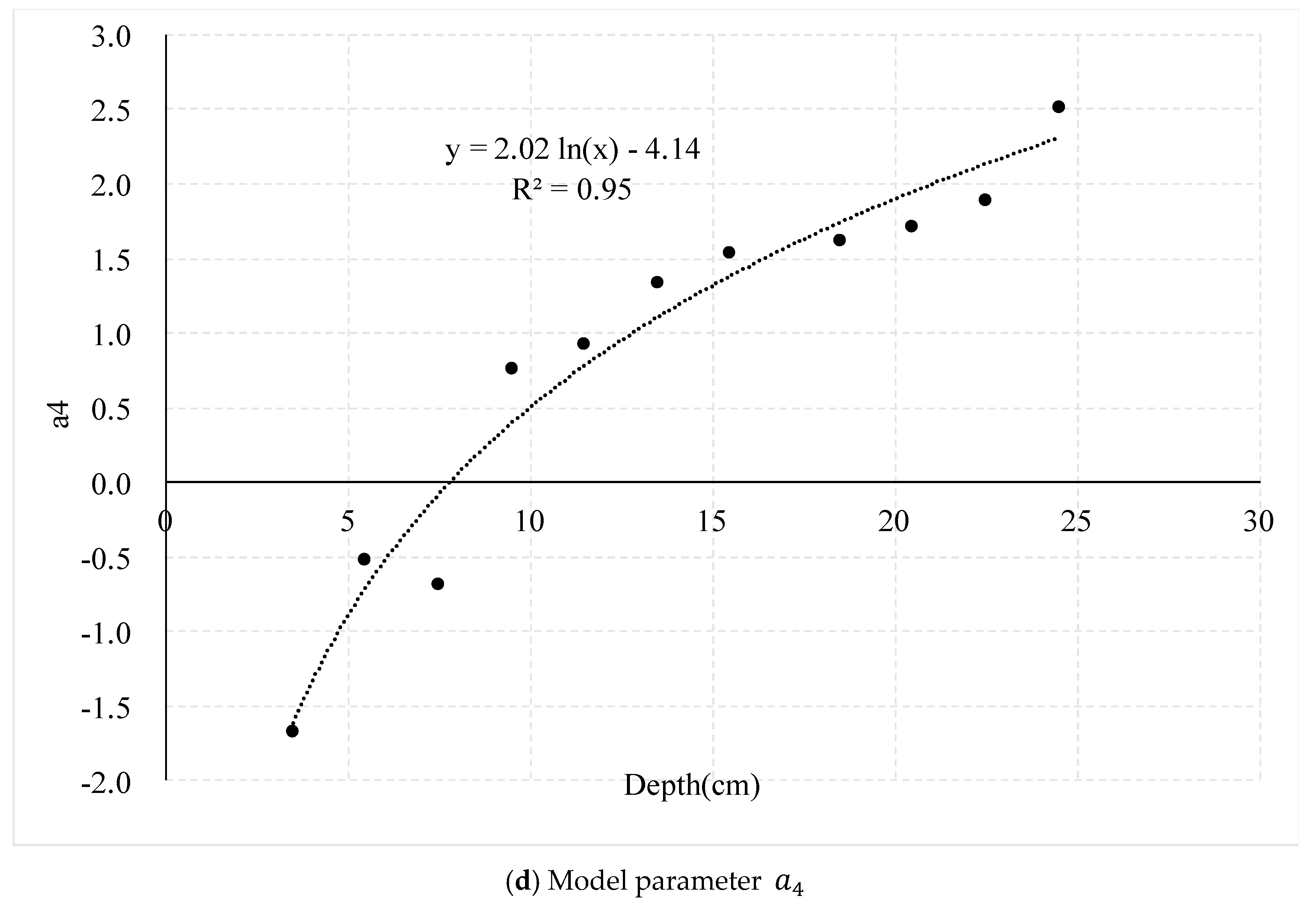
According to the analysis results of Equations (1) and (2), the term significantly affected the estimation of temperature at deeper depths. This research attempted to consider the temperature-transmission effect only by the term as shown in Equation (3). In Equation (3), – are temperature model parameters. The model parameters such as – in Equation (3) for different depths were obtained by performing regression analysis on the temperatures measured at various depths using the least squares method. The analysis results of these parameters are presented in Figure 7, in which , , and are the natural logarithm functions of depth and is approximated to a fixed value—6.564 in this study.
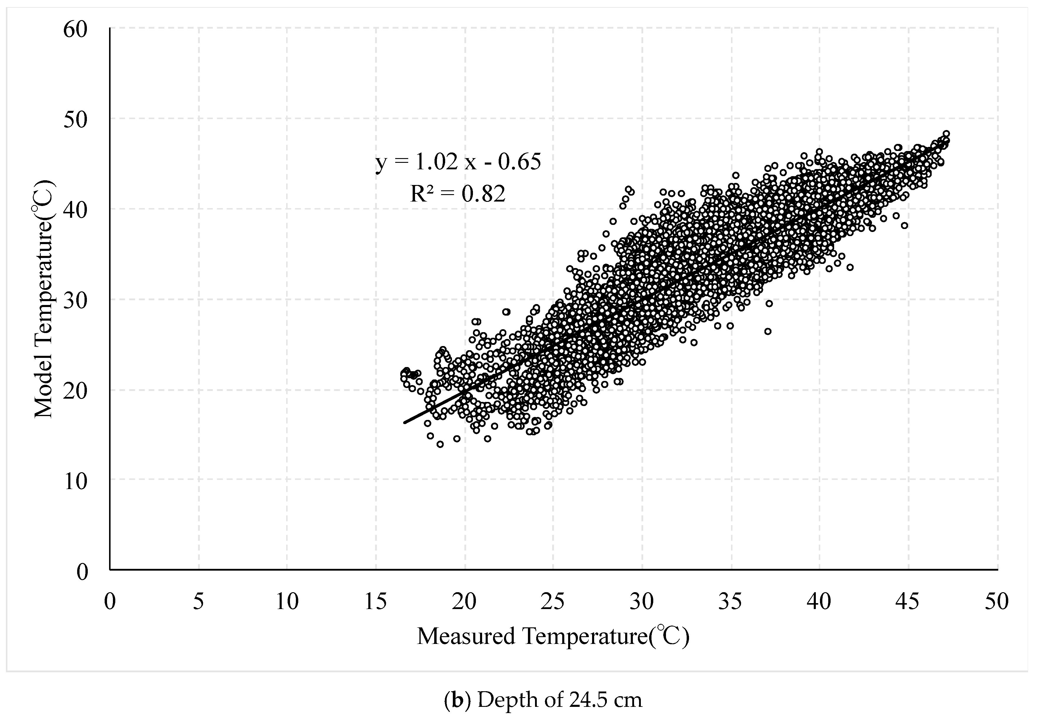
Figure 8 compares the temperatures evaluated by Equation (3) (the model temperature) and the in situ temperature measurements (the measured temperature) for depths of 5.5 and 24.5 cm as examples. Table 4 summarized the results of correlation between measured and model temperature at various depths. The correlation coefficients at depths of 3.5 and 5.5 cm were 0.87 and 0.90, respectively. The correlation coefficient decreased with increasing depth; however, at a depth of 24.5 cm, the correlation coefficient between the model and measured temperatures remained high at 0.82. Moreover, the slopes of regression equation between model and measured temperatures were within 1 ± 0.05, and the intercepts were all within ±2. The results show that the temperature-evaluation model using Equation (3) can reflect the temperature at various depths in the road structure. Furthermore, the model remains effective when estimating the temperature at deep depths. Hence, in order to reduce the model parameter and to have acceptable accuracy of estimated temperature at deep depths, this research employed Equation (3) as the temperature model to estimate the pavement temperature at various depths. The proposed model and obtained parameters – were based on the statistical analysis of temperature measurements in Taiwan. The climate of Taiwan belongs to the subtropics and the lowest and highest atmospheric temperature of the FWD test site are around 6 and 37 °C, respectively. More applications and validations of the model require further temperature measurements and analyses for other weather conditions.
5. Dynamic Modulus Test
To verify the FWD back-calculation with temperature correction, core drilling was performed at the test site. The cored specimens were 10 cm in diameter to satisfy the size requirements of the test specimens in dynamic modulus test. The drilling depth was approximately 35 cm to ensure that both DGAC and BTB were contained. Subsequently, the cored specimens were cut to separate DGAC and BTB, producing DGAC and BTB test specimens of 15 cm in height. However, the surface layers (PAC, OGAC, and SMA) were too thin to meet the height requirement for dynamic modulus testing. Consequently, dynamic modulus tests were only conducted on the DGAC and BTB specimens.
Dynamic modulus tests are widely used to evaluate the influence of temperature and frequency on the properties of asphalt materials. In this study, a material test system was used to perform the dynamic modulus tests at different temperatures and frequencies. The tests were performed at 15 °C, 25 °C, 35 °C, 45 °C, and 55 °C, and frequencies of 25, 10, 5, 1, 0.5, and 0.1 Hz were used for the tests. Figure 9 presents the dynamic modulus test results of DGAC and BTB layers at different temperatures and frequencies. The frequency-temperature superposition principle was employed to form the master curve by horizontal shifting (Figure 9) to the reference temperature 35 °C in this study. A sigmoidal function as shown in Equation (4) was employed to create a master curve of dynamic modulus. In Equation (4), is the reduced frequency, is the frequency-temperature shift factor, is the frequency, is the minimum logarithmic value of , is the maximum logarithmic value of , and are parameters describing the shape of the sigmoidal function.
Table 5 presents the sigmoidal function coefficients for the DGAC and BTB specimens obtained by using the least squares method. Figure 10 illustrates the relationship between the frequency-temperature shift factor and temperature of the DGAC and BTB specimens, whereas Figure 11 displays the master curve of dynamic modulus for the DGAC and BTB specimens at 35 °C. Then, the relationship between frequency-temperature shifted factor and temperature can be formulated as shown in Equations (5) and (6) for DGAC and BTB, respectively. In Equations (5) and (6), is the pavement temperature estimated by the temperature-evaluation model (Equation (3)).
The frequency-temperature shift factor calculated by Equations (5) and (6) is employed to conduct the temperature correction of FWD back-calculation at different temperatures and then the corrected modulus will be compared with master curve (Figure 11) to verify the effectiveness of the temperature correction of back-calculation using the frequency-temperature superposition principle.
6. FWD Back-Calculation and Frequency-Temperature Correction
The layered elastic analysis program LEAF in the BAKFAA back-calculation software [33] was employed in this study to perform back-calculation of the FWD data obtained at the four test road sections. Because the surface layers such as OGAC, PAC, and SMA were functional layers and overly thin, they were combined with DGAC to form a single layer for the convenience of back-calculation and improvement of convergence. In Sections 1 and 2, the OGAC was integrated with DGAC to form a single layer; the OGAC and SMA in Section 3 were integrated with DGAC to form a single layer; and the PAC and SMA of Section 4 were integrated with DGAC to form a single layer. Figure 12 illustrates the adjusted cross-sections used in the back-calculation.
This study considered the loading duration of the FWD as 29 ms, corresponding to an approximate frequency of 17.24 Hz [34]. Since FWD tests were conducted at different temperatures and the modulus of asphalt material layer is related to temperature, the back-calculated modulus of the asphalt layer could not be directly compared with those obtained by the dynamic modulus test. Therefore, the back-calculated modulus values of asphalt layer had to undergo frequency-temperature correction. This study employed the frequency-temperature shift factors obtained by the dynamic modulus test to perform temperature correction for back-calculation at various temperatures.
Figure 13 illustrates the frequency-temperature correction flowchart, while Figure 14 presents a schematic plot of the frequency-temperature correction. Firstly, FWD back-calculation at different temperatures was performed to obtain the modulus of the asphalt material layer represented by the dots in Figure 14. This study used the temperature from the middle of the asphalt material layer and the temperature was evaluated by the temperature model as shown in Equation (3). According to the determined temperature, the frequency-temperature shift factor can be obtained through the dynamic modulus test (Equations (5) and (6)). The back-calculated modulus of the asphalt layer can be shifted by the same amount of obtained frequency-temperature shift factor shown from the dotted line in Figure 14. Through temperature correction, the back-calculated asphalt material layer moduli at different temperatures were shifted to those of the reference temperature, enabling comparison of asphalt material layer moduli obtained by dynamic modulus test.
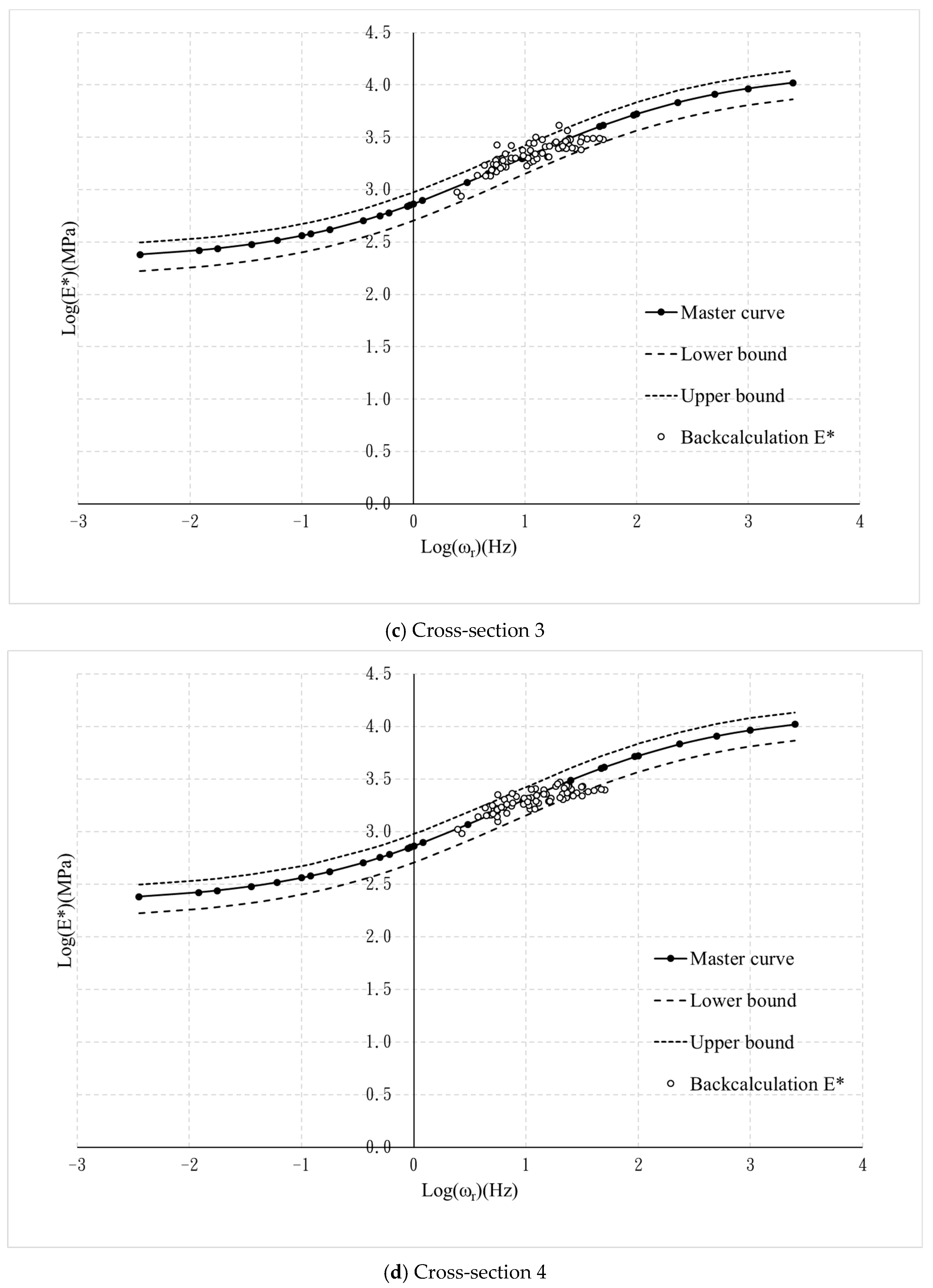
Figure 15 illustrates a comparison of the dynamic modulus master curve of DGAC and the back-calculated modulus of that layer with frequency-temperature correction. The solid line is the master curve of DGAC obtained from the dynamic modulus test, while the dotted lines indicate the ±30% range of the master curve. Table 6 summarizes the percentage of the back-calculated DGAC results that fell within this ±30% range. The results show that the back-calculated modulus of DGAC with frequency-temperature correction had more than 70% within the ±30% range, except for cross-section 1. Figure 16 shows a comparison of the dynamic modulus master curve of the BTB and the modulus values obtained by FWD back-calculation with frequency-temperature correction. Table 7 presents the percentage of back-calculated BTB results that fell within the ±30% range of the dynamic modulus master curve. The results show that more than 85% of back-calculated moduli fell within this range. These results indicate that the proposed frequency-temperature correction can efficiently correct the FWD back-calculated modulus of asphalt material at different temperatures.
By comparing the BTB and DGAC back-calculation results, the BTB results were found to be more accurate than the DGAC results. The reasons can be summarized preliminarily as: (1) The cross-section of the DGAC used in the back-calculation combined several other layers (i.e., OGAC, SMA, and PAC); however, the dynamic modulus master curve of DGAC generated in the laboratory was based on a single material. Hence, the DGAC results were more unsatisfactory than those for the BTB layer. (2) The DGAC was relatively close to the road surface and had a relatively large temperature gradient across its depth. However, the collected temperature adopted for the frequency-temperature correction was simply selected as the temperature at the middle depth of that layer, which could have led to a relatively large error in the DGAC material modulus with frequency-temperature correction.
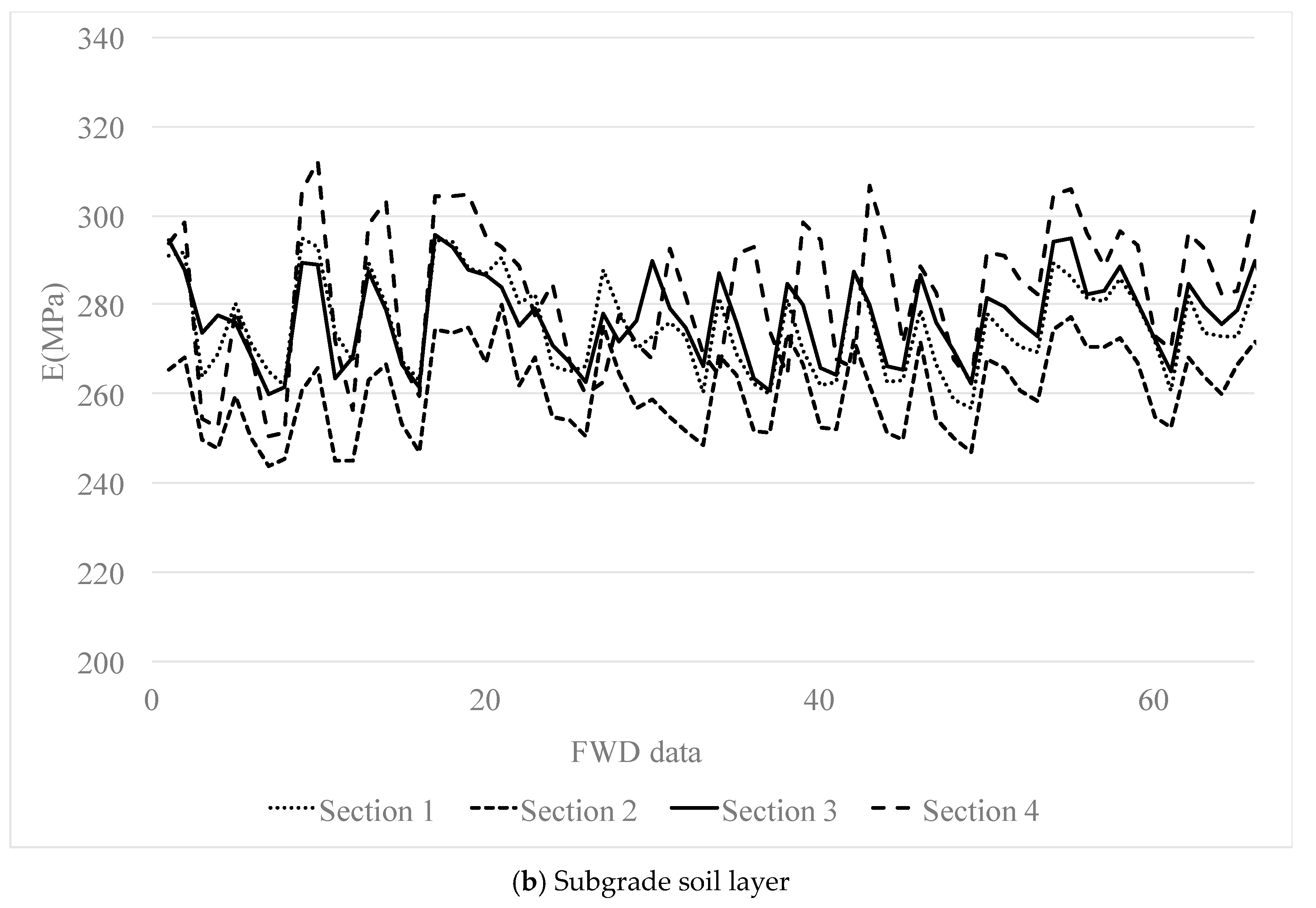
Figure 17 plots the back-calculated modulus of the aggregate subbase layer and subgrade soil layer. The horizontal axis indicates the number of FWD back-calculated data. Since the modulus of the aggregate subbase and soil subgrade are not significantly related to temperature, the frequency-temperature correction does not apply to those layers. The results show the back-calculated modulus of the aggregate subbase in cross-section 4 was consistently considerably lower than that in the other cross-sections. Moreover, the back-calculated modulus of subbase and subgrade in the same section were mostly consistent. These results revealed that FWD tests and back-calculation effectively distinguished the modulus of the four cross-sections and the modulus of the aggregate subbase layer and subgrade soil layer did not strongly influence by temperature, which is in agreement with these materials’ properties.
7. Conclusions and Suggestions
This study proposed a temperature-evaluation model for estimating the temperature at various depth of pavement and conducted the frequency-temperature correction for FWD back-calculation using the frequency-temperature superposition principle. The proposed temperature-evaluation model was developed through the statistical analysis of temperature measurements in a FWD test site. The in situ cored specimens were obtained from the FWD test site and the samples were subjected to dynamic modulus tests in the laboratory to determine the frequency-temperature shift factors and master curves. The FWD back-calculations were performed with frequency-temperature correction and the back-calculated modulus of the asphalt layer was compared with the master curve. The following are the conclusions and suggestions.
- The proposed temperature-evaluation model, considering the effect of temperature-transmission delay, can effectively and reliably estimate the temperature at different depths of the pavement structure. The estimated temperature at deep depth remains reliable when compared with the measured temperature (i.e., R2 = 0.82 at depth of 24.5 cm).
- The frequency-temperature superposition principle was employed to conduct the temperature correction for asphalt material layers. The average percentages of the temperature-corrected back-calculated modulus within ±30% range of the master curve are 71.59% and 89.02% for the DGAC and BTB layers, respectively. This result indicates that the frequency-temperature superposition principle can effectively apply to correct the temperature effect of FWD back-calculation for asphalt layer.
- The back-calculated results of the subbase and subgrade layers show that the moduli of subbase and subgrade are not significantly affected by temperature, which is in agreement with the properties of these materials. The back-calculated modulus of the subbase and subgrade are mostly consistent in the same section.
- The proposed temperature-evaluation model in this research is developed based on only one year and local temperature measurements. More temperature measurements should be included in future research to enhance the accuracy and application of model.
- This research combined several layers (i.e., OGAC, SMA and PAC) with a DGAC layer in back-calculation. In future research, the moduli of the OGAC, SMA, and PAC layers should be obtained in a laboratory through dynamic modulus tests and considered as known moduli in back-calculation to improve the back-calculated results of DGAC.
Author Contributions
Conceptualization, C.-W.H.; methodology, C.-W.H.; software, J.L.; validation, J.L.; resources, J.-C.L.; data curation, J.L.; writing—original draft preparation, J.L.; writing—review and editing, J.-C.L. and C.-W.H. visualization, J.L.; supervision, C.-W.H. and J.-C.L.; project administration, C.-W.H.; funding acquisition, J.-C.L. All authors have read and agreed to the published version of the manuscript.
Funding
This research was funded by Taiwan Freeway Bureau, MOTC, grant number 108C114P009.
Conflicts of Interest
The authors declare no conflict of interest.
References
- Emersleben, A.; Meyer, N. Bearing capacity improvement of asphalt paved road constructions due to the use of geocells—Falling weight deflectometer and vertical stress measurements. In Proceedings of the 4th Asian Regional Conference on Geosynthetics, Shanghai, China, 17–20 June 2008. [Google Scholar]
- Fu, J.; Lei, L.; Liu, Z.; Ma, X.; Zhang, X. Reserve bearing capacity of asphalt pavement based on the reserve factors. In Proceedings of the 2017 4th International Conference on Transportation Information and Safety (ICTIS), Banff, AB, Canada, 8–10 August 2017. [Google Scholar]
- George, K.P. Falling Weight Deflectometer for Estimating Subgrade Moduli; FHWA/MS-DOT-RD-03-153; Department of Civil Engineering, University of Mississippi: Oxford, MS, USA, 2003. [Google Scholar]
- Byrum, C.R. Falling weight deflectometer joint load tests used for direct calculation of pavement joint stiffness. Transp. Res. Rec. 2012, 2306, 95–104. [Google Scholar] [CrossRef]
- Terzi, S.; Saltan, M.; Küçüksille, E.U.; Karaşahin, M. Backcalculation of pavement layer thickness using data mining. Neural Comput. Appl. 2012, 23, 1369–1379. [Google Scholar] [CrossRef]
- Miller, H.; Daniel, J.S.; Eftekhari, S.; Kestler, M.; Mallick, R.B. Research on sustainable pavements: Changes in in-place properties of recycled layers due to temperature and moisture variations. In Proceedings of the International Conference on Highway Pavements and Airfield Technology 2017, Philadelphia, PA, USA, 27–30 August 2017. [Google Scholar]
- Senseney, C.T.; Grasmick, J.; Mooney, M.A. Sensitivity of lightweight deflectometer deflections to layer stiffness via finite element analysis. Can. Geotech. J. 2015, 52, 961–970. [Google Scholar] [CrossRef]
- Ahmed, A.T.; Khalid, H.A. Backcalculation models to evaluate light falling weight deflectometer moduli of road foundation layer made with bottom ash waste. Transp. Res. Rec. 2011, 2227, 63–70. [Google Scholar] [CrossRef]
- Varma, S.; Emin Kutay, M. Backcalculation of viscoelastic and nonlinear flexible pavement layer properties from falling weight deflections. Int. J. Pavement Eng. 2015, 17, 388–402. [Google Scholar] [CrossRef]
- Levenberg, E.; McDaniel, R.S.; Olek, J. Validation of NCAT Structural Test Track Experiment Using INDOT APT Facility; FHWA/IN/JTRP-2008/26; Joint Transportation Research Program: West Lafayette, Indiana, 2008. [Google Scholar]
- Kutay, M.E.; Chatti, K.; Lei, L. Backcalculation of dynamic modulus master curve from falling weight deflectometer surface deflections. Transp. Res. Rec. 2011, 2227, 87–96. [Google Scholar] [CrossRef]
- Park, S.; Kim, Y. Temperature correction of backcalculated moduli and deflections using linear viscoelasticity and time-temperature superposition. Transp. Res. Rec. 1997, 1570, 108–117. [Google Scholar] [CrossRef]
- Straube, E.; Jansen, D. Temperature correction of falling weight deflectometer measurements. In Proceedings of the 8th International Conference on the Bearing Capacity of Roads, Railways and Airfields, Champaign, IL, USA, 29 June–2 July 2009; Volume 2, pp. 789–798. [Google Scholar]
- Wu, S.P.; Xiao, Y.; Liu, Q.T.; Cao, T.W. Temperature sensitivity of asphalt-aggregate adhesion via dynamic mechanical analysis. Key Eng. Mater. 2008, 385–387, 473–476. [Google Scholar] [CrossRef]
- Hossain, M.I.; Tarefder, R.A. Behavior of asphalt mastic films under laboratory controlled humidity conditions. Constr. Build. Mater. 2015, 78, 8–17. [Google Scholar] [CrossRef]
- Lukanen, E.O.; Stubstad, R.N.; Briggs, R. Temperature Predictions and Adjustment Factors for Asphalt Pavement; FHWA-RD-98-085; Office of Infrastructure Research and Development, Federal Highway Administration: Washington, DC, USA, 2000.
- Park, D.-Y.; Buch, N.; Chatti, K. Effective layer temperature prediction model and temperature correction via falling weight deflectometer deflections. Transp. Res. Rec. 2001, 1764, 97–111. [Google Scholar] [CrossRef]
- Park, H.M.; Kim, Y.R.; Park, S. Temperature correction of multiload-level falling weight deflectometer deflections. Transp. Res. Rec. 2002, 1806, 3–8. [Google Scholar] [CrossRef]
- Marshall, C.; Meier, R.; Welch, M. Seasonal temperature effects on flexible pavements in Tennessee. Transp. Res. Rec. 2001, 1764, 89–96. [Google Scholar] [CrossRef]
- Zheng, Y.; Kang, H.; Cai, Y.; Zhang, Y. Effects of temperature on the dynamic properties of asphalt mixtures. J. Wuhan Univ. Technol.-Mater. Sci. Ed. 2010, 25, 534–537. [Google Scholar] [CrossRef]
- Mogawer, W.S.; Austerman, A.J.; Daniel, J.S.; Zhou, F.; Bennert, T. Evaluation of the effects of hot mix asphalt density on mixture fatigue performance, rutting performance and MEPDG distress predictions. Int. J. Pavement Eng. 2011, 12, 161–175. [Google Scholar] [CrossRef]
- Caliendo, C. Local calibration and implementation of the mechanistic-empirical pavement design guide for flexible pavement design. J. Transp. Eng. 2012, 138, 348–360. [Google Scholar] [CrossRef]
- Mai, D.; Turochy, R.E.; Timm, D.H. Sensitivity of flexible pavement thickness to traffic factors in mechanistic-empirical pavement design. J. Transp. Eng. 2014, 140, 04013005. [Google Scholar] [CrossRef]
- Seo, J.; Kim, Y.; Cho, J.; Jeong, S. Estimation of in situ dynamic modulus by using MEPDG dynamic modulus and FWD data at different temperatures. Int. J. Pavement Eng. 2013, 14, 343–353. [Google Scholar] [CrossRef]
- Solatifar, N.; Kavussi, A.; Abbasghorbani, M.; Sivilevičius, H. Application of FWD data in developing dynamic modulus master curves of in-service asphalt layers. J. Civ. Eng. Manag. 2017, 23, 661–671. [Google Scholar] [CrossRef]
- Witczak, M.W.; Fonseca, O.A. Revised predictive model for dynamic (complex) modulus of asphalt mixtures. Transp. Res. Rec. 1996, 1540, 15–23. [Google Scholar] [CrossRef]
- Bari, J.; Witczak, M. Development of A New Revised Version of the Witczak E* Predictive Model for Hot Mix Asphalt Mixtures (with Discussion). In Proceedings of the 2006 Journal of the Association of Asphalt Paving Technologists, Savannah Georgia, GA, USA, 27–29 March 2006; Volume 75, pp. 381–423. [Google Scholar]
- Christensen, D.W.; Bonaquist, R. Improved Hirsch model for estimating the modulus of hot-mix asphalt. Road Mater. Pavement Des. 2015, 16, 254–274. [Google Scholar] [CrossRef]
- Killingsworth, B.; Von Quintus, H. Back-Calculation of Layer Moduli of LTPP General Pavement Study (GPS) Sites; FHWA-RD-97-086; Office of Engineering Research and Development, Federal Highway Administration: Washington, DC, USA, 1997.
- Ye, Y.L.; Zhuang, C.Y.; Zhang, R.F. A method for temperature correction of HMA dynamic modulus. Appl. Mech. Mater. 2012, 178–181, 1615–1618. [Google Scholar] [CrossRef]
- Zhou, L. Temperature correction factor for pavement moduli backcalculated from falling weight deflectometer Test. In CICTP 2014: Safe, Smart, and Sustainable Multimodal Transportation Systems, Proceedings of the 14th COTA International Conference of Transportation Professionals, Changsha, China, 4–7 July 2014; American Society of Civil Engineers: Reston, VA, USA, 2014; pp. 1080–1090. [Google Scholar]
- Chen, D.-H.; Bilyeu, J.; Lin, H.-H.; Murphy, M. Temperature correction on falling weight deflectometer measurements. Transp. Res. Rec. 2000, 1716, 30–39. [Google Scholar] [CrossRef]
- Hayhoe, G.F.; Hughes, W.J. LEAF—A New Layered Elastic Computational Program for FAA Pavement Design and Evaluation Procedures; Federal Aviation Administration: Washington, DC, USA, 2002.
- Pożarycki, A.; Górnaś, P.; Wanatowski, D. The influence of frequency normalization of FWD pavement measurements on backcalculated values of stiffness moduli. Road Mater. Pavement Des. 2017, 20, 1–19. [Google Scholar] [CrossRef] [Green Version]
Figure 1.
Aerial photograph of the test site.

Figure 2.
Top view of the test site.

Figure 3.
Cross-section and the thermometer configuration.

Figure 4.
Thermometers placed at the test site.

Figure 5.
Falling weight deflectometer (FWD) PRIMAX 1500.

Figure 6.
Over-time variation of atmospheric temperature at depths of 3.5 and 24.5 cm.

Figure 7.
The relationship between the parameter of temperature-evaluation model and depth.


Figure 8.
The comparison between measured and evaluated temperature.


Figure 9.
Results of dynamic modulus tests.


Figure 10.
Relationship between temperature and shift factor.


Figure 11.
Dynamic modulus master curve.


Figure 12.
Schematic of layers used in back-calculation analysis.

Figure 13.
Temperature correction procedures.

Figure 14.
Schematic of temperature correction.

Figure 15.
Comparison between the dynamic modulus master curve and FWD back-calculated results for DGAC layer.
Figure 15.
Comparison between the dynamic modulus master curve and FWD back-calculated results for DGAC layer.


Figure 16.
Comparison between the dynamic modulus master curve and FWD back-calculated results for BTB layer.
Figure 16.
Comparison between the dynamic modulus master curve and FWD back-calculated results for BTB layer.


Figure 17.
The back-calculated results of subbase and subgrade layer for cross sections 1–4.


Table 1.
Asphalt binder type and percentage of binder content.
| Asphalt Material | Asphalt Cement | Asphalt Binder Content |
|---|---|---|
| DGAC | AC-20 | 5.0% |
| OGAC | AC-20 | 5.0% |
| PAC | Type-III modified | 5.1% |
| SMA | Type-III modified | 6.3% |
| BTB | AC-20 | 4.5% |
Table 2.
Correlation between measured and estimated temperature for various depths.
| The Estimated Temperature of Equation (1) | The Estimated Temperature of Equation (2) | |||||
|---|---|---|---|---|---|---|
| Depth | R2 | Slope | Intercepts | R2 | Slope | Intercepts |
| 3.5 cm | 0.88 | 1.13 | −4.41 | 0.88 | 0.95 | 1.98 |
| 5.5 cm | 0.83 | 1.05 | −1.72 | 0.90 | 1.00 | 0.26 |
| 7.5 cm | 0.80 | 0.95 | 1.13 | 0.89 | 0.99 | 0.47 |
| 9.5 cm | 0.74 | 0.88 | 3.01 | 0.89 | 0.99 | 0.18 |
| 11.5 cm | 0.69 | 0.82 | 4.50 | 0.88 | 0.99 | 0.25 |
| 13.5 cm | 0.62 | 0.62 | 6.18 | 0.88 | 1.00 | 0.04 |
| 15.5 cm | 0.61 | 0.76 | 6.23 | 0.86 | 0.99 | 0.07 |
| 18.5 cm | 0.56 | 0.73 | 7.20 | 0.86 | 0.98 | 0.66 |
| 20.5 cm | 0.54 | 0.74 | 6.71 | 0.82 | 1.00 | 0.24 |
| 22.5 cm | 0.53 | 0.75 | 6.35 | 0.82 | 1.00 | 0.09 |
| 24.5 cm | 0.53 | 0.77 | 5.36 | 0.82 | 1.02 | −0.60 |
Table 3.
Coefficient of correlation between atmospheric and pavement temperature at various depths for various delay times.
Table 3.
Coefficient of correlation between atmospheric and pavement temperature at various depths for various delay times.
| Delay Time | 0 h | 1 h | 2 h | 3 h | 4 h | 5 h | 6 h | |
|---|---|---|---|---|---|---|---|---|
| Depth | ||||||||
| 3.5 cm | 0.857 | 0.872 | 0.806 | 0.684 | 0.535 | 0.387 | 0.261 | |
| 5.5 cm | 0.816 | 0.887 | 0.881 | 0.809 | 0.691 | 0.553 | 0.416 | |
| 7.5 cm | 0.790 | 0.876 | 0.892 | 0.843 | 0.744 | 0.616 | 0.483 | |
| 9.5 cm | 0.750 | 0.849 | 0.889 | 0.867 | 0.792 | 0.683 | 0.558 | |
| 11.5 cm | 0.714 | 0.819 | 0.876 | 0.875 | 0.823 | 0.731 | 0.618 | |
| 13.5 cm | 0.640 | 0.759 | 0.841 | 0.873 | 0.853 | 0.790 | 0.697 | |
| 15.5 cm | 0.642 | 0.748 | 0.824 | 0.857 | 0.844 | 0.790 | 0.707 | |
| 18.5 cm | 0.600 | 0.704 | 0.788 | 0.837 | 0.846 | 0.816 | 0.754 | |
| 20.5 cm | 0.536 | 0.631 | 0.717 | 0.781 | 0.814 | 0.813 | 0.781 | |
| 22.5 cm | 0.516 | 0.603 | 0.686 | 0.752 | 0.791 | 0.801 | 0.781 | |
| 24.5 cm | 0.489 | 0.568 | 0.646 | 0.713 | 0.759 | 0.780 | 0.773 | |
Table 4.
Correlation between measured and estimated temperature at various depths.
| Depth (cm) | R2 | Slope | Intercept |
|---|---|---|---|
| 3.5 | 0.87 | 0.96 | 1.91 |
| 5.5 | 0.90 | 1.01 | 0.03 |
| 7.5 | 0.89 | 1.00 | 0.18 |
| 9.5 | 0.89 | 1.00 | −0.15 |
| 11.5 | 0.88 | 1.00 | −0.07 |
| 13.5 | 0.87 | 1.00 | −0.25 |
| 15.5 | 0.86 | 1.00 | −0.20 |
| 18.5 | 0.86 | 0.99 | 0.45 |
| 20.5 | 0.83 | 1.00 | 0.11 |
| 22.5 | 0.83 | 1.00 | 0.00 |
| 24.5 | 0.82 | 1.02 | −0.64 |
Table 5.
Parameters of sigmoidal function for dense-graded asphalt concrete (DGAC) and bitumen-treated base (BTB) analysis.
Table 5.
Parameters of sigmoidal function for dense-graded asphalt concrete (DGAC) and bitumen-treated base (BTB) analysis.
| DGAC | BTB | |
|---|---|---|
| δ | 2.210 | 2.320 |
| α | 1.774 | 1.821 |
| β | 0.687 | 0.858 |
| γ | −1.143 | −1.033 |
Table 6.
Range distribution of the back-calculated results for the DGAC layer.
| DGAC | ||||
|---|---|---|---|---|
| Section 1 | Section 2 | Section 3 | Section 4 | |
| Number of data | 66 | 66 | 66 | 66 |
| Number of data within 30% | 30 | 48 | 56 | 55 |
| Percentage of data within the range | 45.45% | 72.73% | 84.85% | 83.33% |
Table 7.
Range distribution of the back-calculated results for the BTB layer.
| BTB | ||||
|---|---|---|---|---|
| Section 1 | Section 2 | Section 3 | Section 4 | |
| Number of data | 66 | 66 | 66 | 66 |
| Number of data within 30% | 58 | 58 | 60 | 59 |
| Percentage of data within the range | 87.88% | 87.88% | 90.91% | 89.39% |
© 2019 by the authors. Licensee MDPI, Basel, Switzerland. This article is an open access article distributed under the terms and conditions of the Creative Commons Attribution (CC BY) license (http://creativecommons.org/licenses/by/4.0/).
Share and Cite
MDPI and ACS Style
Lai, J.-C.; Liu, J.; Huang, C.-W. The Application of Frequency-Temperature Superposition Principle for Back-Calculation of Falling Weight Deflectometer. Appl. Sci. 2020, 10, 132. https://0-doi-org.brum.beds.ac.uk/10.3390/app10010132
AMA Style
Lai J-C, Liu J, Huang C-W. The Application of Frequency-Temperature Superposition Principle for Back-Calculation of Falling Weight Deflectometer. Applied Sciences. 2020; 10(1):132. https://0-doi-org.brum.beds.ac.uk/10.3390/app10010132
Chicago/Turabian StyleLai, Jung-Chun, Jung Liu, and Chien-Wei Huang. 2020. "The Application of Frequency-Temperature Superposition Principle for Back-Calculation of Falling Weight Deflectometer" Applied Sciences 10, no. 1: 132. https://0-doi-org.brum.beds.ac.uk/10.3390/app10010132
Note that from the first issue of 2016, this journal uses article numbers instead of page numbers. See further details here.