Article

Operational USLE-Based Modelling of Soil Erosion in Czech Republic, Austria, and Bavaria—Differences in Model Adaptation, Parametrization, and Data Availability

1
Working Group Water and Soil Resource Research, Institute of Geography, University of Augsburg, 86159 Augsburg, Germany
2
Department of Landscape Water Conservation, Faculty of Civil Engineering, Czech Technical University in Prague, 160 00 Prague, Czech Republic
3
Federal Agency for Water Management, Land and Water Management Research, 1040 Vienna, Austria
4
Department of Environmental Systems Science, Eidgenössische Technische Hochschule Zürich, 8092 Zurich, Switzerland
*
Author to whom correspondence should be addressed.
Submission received: 27 April 2020 / Revised: 19 May 2020 / Accepted: 21 May 2020 / Published: 25 May 2020
(This article belongs to the Special Issue Challenges and Solutions in Soil and Water Conservation)

Abstract

:
In the European Union, soil erosion is identified as one of the main environmental threats, addressed with a variety of rules and regulations for soil and water conservation. The by far most often officially used tool to determine soil erosion is the Universal Soil Loss Equation (USLE) and its regional adaptions. The aim of this study is to use three different regional USLE-based approaches in three different test catchments in the Czech Republic, Germany, and Austria to determine differences in model results and compare these with the revised USLE-base European soil erosion map. The different regional model adaptations and implementation techniques result in substantial differences in test catchment specific mean erosion (up to 75% difference). Much more pronounced differences were modelled for individual fields. The comparison of the region-specific USLE approaches with the revised USLE-base European erosion map underlines the problems and limitations of harmonization procedures. The EU map limits the range of modelled erosion and overall shows a substantially lower mean erosion compared to all region-specific approaches. In general, the results indicate that even if many EU countries use USLE technology as basis for soil conservation planning, a truly consistent method does not exist, and more efforts are needed to homogenize the different methods without losing the USLE-specific knowledge developed in the different regions over the last decades.

1. Introduction

Soil erosion, in the context of arable land use, is one of the major threats for global soils [1,2] resulting in on-site and off-site damage [3]. On-site effects range from a reduction in crop yields [4,5] to a decrease in soil organic carbon storage [6], while typical off-site effects are the eutrophication of inland waters [7] as well as silting of reservoirs [8].
In the European Union, soil erosion is identified as one of the main environmental threats (see EU commission thematic strategy soil). It is addressed in a variety of rules and regulations associated with different soil and water protection targets, which are focused on on-site soil conservation. The prevention of on-site damages has the main aim to fulfil the requirements of ’Good Agriculture and Environmental Condition’ (GAEC) [9] as defined in the framework of the so-called Cross-Compliance [10], while the prevention of off-site damages mainly aims to reach the targets of the Water Framework Directive [11]. In this context, the interplay between a number of farming regulations and potential financial support provided to farmers via the EU (Cross-Compliance approach) is of tremendous importance as part of the Common Agricultural Policy (CAP). Within the EU legal framework, each country has a certain level of flexibility in the way grant payments to farmers are organized while taking national conditions into account. The same holds true for tools used to determine the effects of certain farming practices, e.g., for soil conservation. In the fields of erosion risk assessment, the used tools differ substantially between the EU countries or even between regions within countries. For example, in Germany, the federal state of Bavaria is using the German adaption of the Universal Soil Loss Equation (USLE) [12] which is the basis of a German Industry Standard [13], while the federal state of Saxony is using the physically-based model EROSION3D [14]. In general, the USLE [15,16] and the revised USLE (RUSLE; [17]) and its national and regional adaptions, partly resulting from specific data availability, are the most widely used tools for erosion risk assessment in Europe [18].
Apart from the different national and regional adaptations of the USLE and/or RUSLE, there is a recent RUSLE-based European Soil Erosion Map [19], which used more generalized data available at a European level. This is supposed to allow for a regional comparison but is hardly applicable on the scale where soil conservation can be set into practice—the single parcel, or even specific parts of it. However, as no homogeneous soil erosion map or mapping technique was established at this level, which can be used to establish soil conservation strategies and allocate European or national/regional funds as incentives for farmers, one has to deal with potentially large differences in mathematical description/modelling approaches and model implementations of the same model (mostly the USLE and derivatives) in individual European countries or administrative units.
The aim of this study is to use three different regional USLE-based approaches in three different test catchments in the Czech Republic, in Germany in the federal state of Bavaria (in the following referred to as Bavaria), and Austria, where nation-specific methods of soil loss calculations will be cross applied to (i) determine differences in modelled erosion due to the different model implementation, (ii) analyze and determine the most sensitive differences, and (iii) illustrate the difference between national USLE-based erosion risk maps and more generalized USLE-based European soil erosion risk map.

2. Materials and Methods

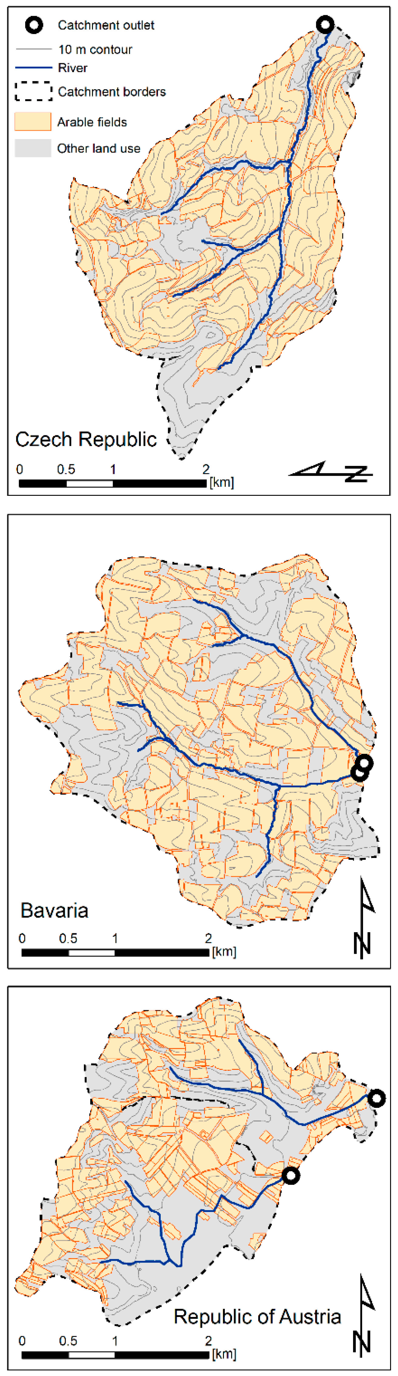
2.1. Test Catchments

The effects of different USLE implementations as officially used in the Czech Republic (CZ), Austria (AT), and Bavaria (BY) were analyzed in three catchments (CZ: 7.8km2, AT: 7.3 km2; BY: 10.1 km2). The catchments were selected on the basis of similarity of size, share of arable land, and geomorphological baseline conditions (i.e., slope). All catchments are under intensive arable use representing typical erosion prone areas in all three regions (Figure 1 and Table 1). Mean annual temperature and mean precipitation difference between the sites are relatively small ranging from 7.7 to 9.0 °C and 739 to 844 mm, respectively. All sites have the most intense rainfall events associated to convective rainfall in summer. All sites are dominated by Cambisols [20], whereas the soils at the Bavarian and Austrian site are mainly loamy, while the soils in the site in the Czech Republic are predominantly sandy loam. Land management differs substantially with largest proportions of small grains (mostly wheat) in the Czech Republic, Bavaria and Austria (83.8%, 53.1%, and 46.5%, respectively). Row crops are with about 45% more dominant in the loams found in Bavaria and Austria compared to about 13% row crops in the sandy loams in the Czech Republic. A major difference between sites are the field sizes, with about 3-times larger fields in the Czech Republic compared to the sites in Bavaria and Austria. This main difference mirrors the different historical developments in land management and land ownership [21]. For more details regarding site characteristics see Table 1 and Figure 1.

2.2. Modelling

In general, the Universal Soil Loss Equation (1) [15] in its national adaptations as operational in 2019 is used in all three regions. Apart from the USLE implementations performed in this study, results are compared to the results derived from the harmonized USLE approach for Europe as presented by Panagos et al. [19]. For the Bavarian site, the USLE as originally adapted by Schwertmann et al. [12] is used, which later on was further refined in the German industry standard DIN 19708 [13]. In the Czech Republic, the USLE, in its original form, has been used linked to distributed GIS-supported approach with individual USLE factors specified by a national Soil Erosion Control Methodology [22]. In Austria, the RUSLE approach is used with some region-specific procedures to determine the USLE factors (see below). All USLE approaches produce potential erosion, so a rigid testing against measured catchment erosion is hardly possible. Hence, it is important to note that there is some underlying assumption that each regional USLE approach performs best in the region of its adaptation. Nevertheless, due to the missing validation against catchment data we purely compare results without judging which model approach performs best.
A = R · K · L · S · C · P,
where A is long-term mean soil loss [t ha−1 a−1]; R is the rainfall and surface runoff factor [N h−1], K is the soil erodibility factor [t h ha−1 N−1], L is the slope length factor [-], S is slope factor [-], C [-] is the soil cover and management factor, and P [-] is the soil protection factor.
Following the official regulations in the Czech Republic, Austria, and Bavaria, the factors of the USLE are calculated as follows, whereas a focus is set to differences in methods:

2.2.1. R Factor

CZ: The R factor is calculated following the original USLE approach [16]. In this procedure rainfall events are subdivided if there is at least a rain gap (with less than 1.27 mm rainfall) of 6 h, and erosive events are defined as events with at least 12.7 mm of rainfall or a minimum 15 min intensity of at least 25.4 mm h−1. To derive the rainfall erosivity map, high resolution rainfall (1 min) of recent 10 years of official Czech Hydro-meteorological Institute digital gauge stations is used. The rainfall erosivity maps in different areas of applications in the Czech Republic differ [23]. For the official USLE soil loss tolerance map used in the context of cross compliance, the calculated mean R factor of the 10 year period is reduced by 40%, based on the comparison of R factors of original pluviometer data and digital rain gauges in an overlapping training period (decision of Ministry of Agriculture/Ministry of Environment of Czech Republic).
To apply the CZ approach in BY and AT, high resolution rainfall data from a meteorological station in the surrounding of the BY test catchment (about 5km apart) and within the AT test catchment were used.
BY: To derive the R factor following Bavarian regulations, a regression between annual precipitation (PA) and rainfall erosivity is used that is documented in the German Industry Standard 19708 [13]. The regression equation (R factor = 0.0833 × PA + 1.73; R 2 = 0.94) was derived from annual precipitation and calculated R factors from 18 stations in Bavaria using 10 years of precipitation data with a temporal resolution of 1 min rainfall (period: 1967 and 1976) [24]. The R factor calculations follow Schwertmann et al. [12], which are based on the original USLE approach [16]. However, the definition of erosive events was slightly adapted to German conditions. Erosive events are defined as events with at least 10 mm of rainfall or a minimum 30 min intensity of at least 10 mm h−1 [12,13]. The mean annual rainfall, needed to derive mean annual rainfall erosivity for the catchment in Bavaria, is taken from a product of the German Weather Service (DWD) providing yearly data for the time span 1981–2010 in a 1 × 1 km2 grid, which was interpolated from station data of the DWD and from neighboring counties stations taking elevation into account [25]. The resulting 1 × 1 km2 erosivity map is aggregated to give a mean erosivity for each municipality.
To apply the BY approach in CZ and AT, the mean long-term annual precipitation (2000–2013 and 1986–2016, respectively) from both sites was utilized.
AT: Similarly to Bavaria, in Austria, a regression relationship between long-term annual rainfall or summer rainfall from April to October (Pveg) and R factor values was developed in the mid 1990s [26] using a similar rain event definition (> 10 mm event rainfall or > 10 mm h−1 event intensity and termination of events after >6 h without rainfall). Recently, this procedure has been refined and updated with recent data sets. While in the original data set 33 rainfall stations were used, the new approach used for this study employs 171 stations (R factor = 0.21 × Pveg − 26.5; R2 = 0.71). For the relationship between rainfall intensity and kinetic energy of rain the equation of van Dijk et al. (2002) is used. To calculate the interannual distribution of R factors needed for the C factor of the RUSLE, R factor distributions were aggregated on the level of main agricultural production zones [27].
To apply the AT approach in BY and CZ, the raster based long-term annual rainfall data from Germany [23] and long-term annual rainfall data from a nearby station at the CZ catchment were used.

2.2.2. K Factor

CZ: For the Czech Republic, the spatially most detailed soil map is a soil bonity map (scale 1:5000) developed since the 1960s and continuously updated, since the map is a basis for the state land tax policy of agricultural land. The map is officially distributed by the State Land Office, and basic soil physical properties are allocated to each bonity unit. For official erosion modelling (cross compliance, land consolidation projects, etc.), a transfer scheme to derive K factor information from the national bonity map was developed [28]. The lookup table used in this transfer scheme is published in the official CZ USLE methodology [29].
BY: In general, the Bavarian administration calculates the K factor following the German Industry Standard DIN 19708 [13], which uses an equation system [30,31] accounting for the full range of the original K factor nomograph as given in Wischmeier et al. [32] and Wischmeier and Smith [16]. The transferability of the original K factors developed for US soils to German soil conditions was extensively tested by Schwertmann et al. (1987), concluding that the US K factors are well applicable for German soils. However, for pragmatic reasons and due to the challenges to provide all necessary soil input data, the German soil bonity map (scale: 1:25,000, for details see Table 2) available for all arable land in Germany is used together with a lookup-table provided in the Industry Standard (DIN 2017). This map provides soil texture as well as information regarding soil genesis and general soil status for agricultural use, all three parameters are used to derive K factor values. The relation between the soil bonity map units and the K factors were originally established by Schwertmann et al. (1987) comparing calculated K factors with map units.
AT: In Austria, K factor values are calculated based on soil silt content (K factor = 0.0083 + Silt% × 0.0086, R 2 = 0.83, n = 30) adjusted to soil surface stone content [33]. This relationship was derived from an evaluation of rainfall simulation experiments and was described in Strauss et al. [34].
As the K factor calculations in each region are based on region-specific data sources, e.g., the CZ bonity map is used with a look-up table to derive K factors from bonity units [29], it was not possible to apply the methods from the other regions in all catchments. Hence, one K factor derived from the regional method of each specific catchment is used in all three USLE implementations.

2.2.3. LS Factor

CZ: In Czechia, the L and S factor is derived only for agricultural land (excluding forests and paved areas). The agricultural land for LS computation is defined by a digital map layer of the Land Parcel Identification System [35]. Before calculating the L factor, all neighboring parcels without any other land use in-between (trails, field road, etc.) are arranged in unified field blocks. Slope length is hence not affected by adjacent field borders. For each unified field block the L and S factor are calculated following the approach of Desmet and Govers [36] using the Usle2D tool provided by the KU Leuven [36,37] with the equation of McCool [38,39] and moderate rill/inter-rill ratio. Multiple flow routing (MFR) is applied for definition of contributing areas.
BY: Following the approach used in Bavaria, the L and S factor is solely derived for arable land. Before calculating the L factor, all neighboring fields without any other land use in-between are arranged in field blocks. For each field block, the L and S factor is calculated using the Usle2D tool [36,37] with the equation of Nearing [40] and the slope length exponent following Wischmeier and Smith [16]. MFR is applied for definition of contributing areas.
AT: For the estimation of L and S factors following the calculation method used in Austria, only cultivated plots are considered for computation in order to simulate overland water flow that is interrupted by linear features (e.g., roads) or suspended by plots that are not assigned as cultivated. The two-dimensional method presented in Desmet and Govers [36] with a slope length exponent m after McCool et al. [41] and the MFR algorithm by Quinn et al. [42] were used for the spatial L factor computation. The S factor was calculated according to Nearing [40].

2.2.4. C Factor

CZ: The C factor values were determined for the presented study using the “Soil Erosion Control Calculator” [43], developed and operated by the Research Institute of Soil and Water Conservation for Ministry of Agriculture and to standardize determination of crop cover effect in soil erosion conservation. The application is publicly available and allows to determine the C factor for a given crop rotation or an individual crop. According to geographic location, the application also suggests an optimum term of individual agrotechnical operations. The calculator has been used by individual farmers to determine relevant crops and crop rotations to fulfil requirements of Cross-Compliance policy defined as ’Good Agriculture and Environmental Condition’ in the Czech Republic. For this study, we selected individual crops identified within the experimental catchment and calculated their C factor values for standard technology of cultivation used in the area [22]. It combines the regional seasonality of erosivity with regional statistical data of planting and harvesting and prescribed soil cover of crops in five development periods as described in Wischmeier and Smith [16]. C factor values for crop rotation has then been calculated as weighted average for crops produced within the area.
BY: The calculation of the C factor follows an approach developed by Auerswald [44] which allows to use the proportion of different crops within a catchment to derive a mean C factor for all arable land within the catchment, without the necessity of crop rotation and seasonal erosivity data. Auerswald [43] calculated C factors based on the seasonality of R factors and cover of more than 200 different crop rotations (including specific management, harvesting dates, etc.) following the approach of Schwertmann et al. (1987). Based on a Monte-Carlo simulation randomly using subsets of the different crop rotations, whereas C factors were calculated before, Auerswald [44] could show that an empirical equation using the test catchment specific proportion of small grains, root crops, root crops under mulch tillage, and perennial crops is suitable to estimate the C factor (R2 = 0.88; p < 0.001; Auerswald 2002).
AT: In Austria, the calculation of C factors is carried out with typical management data for each agricultural production zone. Management data (planting dates, harvest dates, dates and types of management operations) are taken from regional surveys and personal interviews, and the development of plant cover and plant height is derived from model simulations of the soil-water-plant model SIMWASER [45,46]. The algorithms to calculate C factors then strictly follow the procedures of the RUSLE [47].

2.2.5. P Factor

The soil protection P factor of the USLE is set to a single value in all test catchments, following the recommendations of the different administrative units. In the Czech Republic and Austria, soil protection via specific soil conservation management is ignored, and the P factor is always set to 1.0. In Bavaria, a P factor of 0.85 is generally applied, which is based on an analysis of soil protection measures in Bavaria.

2.3. Data

Depending on the region, different data are used as inputs for the different regional USLE approaches. Based on data availability and also for pragmatic reasons, the regional approaches sometimes use specific data-driven adaptations of the USLE, e.g., using available soil bonity maps to derive the K factor (in CZ) instead of deriving it from texture, soil organic carbon data, etc. (in AT and BY) (Table 2). This makes it at times difficult to transfer regional USLE approaches to other regions.
Some data are freely available, but others can only be obtained in cooperation with and/or with specific permission of data providers (Table 2). For the test catchments, all necessary data are available, but especially for the K factor, it was not possible to exchange methods due to a lack of basic soil data. Therefore, K factor values available for all catchments from the regional USLE implementation were used in all other USLE implementations of this study.
The comparison of the three different regional methods against the RUSLE-based EU erosion map [19] was aggregated on soil erosion field means. To yield sound spatially weighted mean values of small fields that only partly cover grid cells, the EU erosion map was resampled from 100 m × 100 m to 5 m × 5 m using a nearest neighbor assignment that resizes the grid resolution while keeping the original values unchanged.

3. Results and Discussion

The modelled soil erosion using the three different USLE approaches in all three test catchments resulted in substantially different overall erosion (Figure 2) and field-specific erosion patterns (Figure 3; Figure 4) between the different methods, while the mean erosion (over all methods) between the test catchments show substantial, but smaller differences (mean BY, AT, and CZ: 13.2, 17.7, and 10.4 t ha−1 a−1, respectively). The highest erosion rates at the Austrian site mostly result from the large proportion of row crops (45.6%), especially maize, without specific soil conservation measures (Table 1).
In general, the lowest modelled mean erosion for all catchments can be found applying the Bavarian method, followed by the Czech and Austrian approaches (Figure 2 and Table 3). The modelled mean erosion over all agriculturally used raster cells in the different catchments using the BY approach was 54% and 59% smaller than CZ and the AT approaches, respectively.
While there is no systematic effect of field size on modelled erosion at the BY and AT test catchments (Figure 4F,K), which are characterized by a large number of relatively small fields (Table 1), there is a tendency that erosion at the CZ site increases with increasing field size (Figure 4C).
In the Czech catchment, the BY method shows a systematic bias in field-specific erosion compared to the CZ methods. Relative differences in field-specific erosion between these methods increase with field size (Figure 4B). In contrast, no clear effect of field size and/or field erosion could be identified comparing the AT with the CZ method (Figure 4C).
In the Bavarian catchment, more pronounced relative differences in field-specific erosion between the CZ and AT method as compared to the BY method were found (Figure 4E,G). With the CZ method, the largest relative deviations from the BY method were identified for small fields (Figure 4E), while for the somewhat larger fields, there is a more or less constant relative difference. Interestingly, relative differences in field erosion between the AT and the BY method indicate much more field specific variability (Figure 4G).
In the Austrian catchment, the largest relative differences between the CZ and BY vs. AT method occurred for small fields with low erosion (approx. < 2 t ha−1 a−1; Figure 4I,J). It is interesting to note that the difference in site-specific mean/median erosion (Figure 2; Table 2) as well as the relative difference (Figure 4G,J) between BY and AT methods are much smaller in case of the AT catchment compared to the BY catchment.
It is obvious from the results shown above that even if all regional/national erosion approaches in principal use USLE-based technology [16], the regional adaptation of the model (as done for Bavaria by Schwertmann et al. [12]), the specific parameterization and technique to derive individual USLE factors, and the differences in available data, result in substantial differences in model results. We identified some bias between the mean field erosion resulting from the different methods but, moreover, found large differences in modelled erosion of individual fields.
As the different USLE approaches were regionally adapted, we assume that the approach adjusted for a specific region performs best in the corresponding region. Therefore, the field-specific results of the different approaches are always presented against the results of the regionally adapted approach (Figure 4). To validate the model results in the three test regions against data to prove our assumption is not/hardly possible. It is important to note that the USLE only produces gross erosion for each raster cell, while transport and deposition are not modelled. Hence, any kind of traditional model validation on a catchment scale using sediment delivery data (e.g., [48]) or catchment internal net soil loss (accounting for soil erosion and deposition in each raster cell), i.e., derived from fallout radionuclides (e.g. [49]) or changes in digital elevation models (e.g., [50]), are generally not feasible. Therefore, our assumption of best regional model performance following regional adaptation is purely supported by plot scale validation in earlier studies (e.g., USLE adaptation for Bavaria [13] or K factor adaptation for Austria [34]).

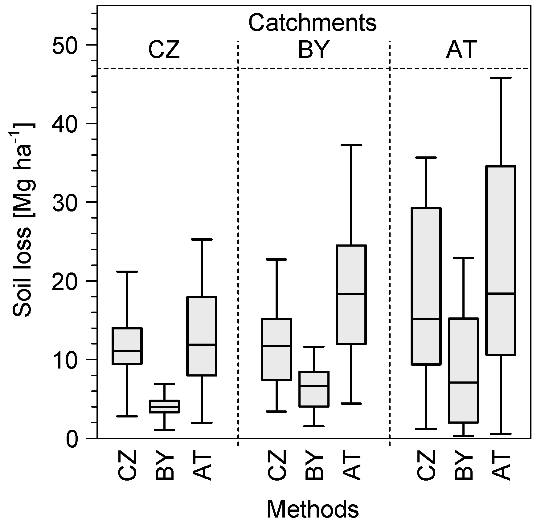
3.1. National Differences Based on USLE Input Parameters

The differences in mean or median erosion for the different sites and methods and the field specific differences result generally from different calculations of the USLE factors and in case of the field differences their spatial distribution. For the R factor, it is first of all the differences in defining erosive events. While the BY and AT methods define the first criterion of an erosive event as events with more than 10 mm rainfall (following the Bavarian USLE adaptation by Schwertmann et al. [12]), the CZ method uses the original threshold of 12.7 mm [16]. Differences in the definitions of the second criterion for an erosive event are even larger (minimum 15 min intensity of at least 25.4 mm h−1, minimum 30 min intensity of at least 10 mm h−1, and minimum intensity of 10 mm h−1 for CZ, BY, and AT, respectively). This is only the first substantial difference which is the basis for very different techniques used to calculate site specific R factors. A further substantial difference is that in BY and AT, a regression between R factors, derived from a limited number of stations and for different historic periods, and mean annual or mean summer rainfall are used to calculated R factors for lager areas or more recent periods. In contrast, the R factor in CZ is calculated directly from high resolution rainfall data (1 min) of the Czech Hydro-Meteorological Institute, which in principal should be more precise than using R-precipitation-relations. In general, both methods to calculate test catchment specific R factors have advantages and disadvantages: Deriving R factors via regressions from annual rainfall is much easier as gridded yearly rainfall data are often easily available and well quality-checked (including the used interpolation techniques) by national weather services (e.g., [25]). The problem might be that the regressions between historic rainfall erosivity data (partly from the 1960s to the 1970s; BY) and annual rainfall might not be stable under changing erosivity due to climate change [51,52]. The disadvantage of the more precise direct calculation of R factors is that spatially distributed data need to be derived using spatial interpolation techniques, which might be weak compared to the gridded data of annual rainfall from weather services, which take elevation, instrument changes, etc. into account [25]. There are newer developments using corrected rainfall radar data (spatial and temporal resolution 1 km × 1 km and 5 min) to derive rainfall erosivity [53] which could be operationally used in USLE-based erosion modelling. However, this will not help in a first attempt to harmonize the R factor calculations in Europe. Given the size of the test catchments, a potentially varying R factor within the catchments is anyway small and hence will not substantially affect field-specific differences in erosion from the different methods.
Another substantial source of differences in modelled mean field erosion are the different approaches to derive the C factor, which varies up to a factor of 2.8 between methods (Table 3). All calculations refer to USLE methodology whereas the seasonality in soil cover from different crops is combined with seasonality of the R factor. However, for practical reasons, this time-consuming and data-intensive approach is then either simplified and empirical equations to derive C factors for specific crop rotations implemented [44], or even more complex models are used to first of all create a seasonality of soil cover [45] before using RUSLE procedures [47]. These different approaches might fit perfectly for the different regions but would require more testing before transferring from one region to another. A main reason for the larger variability in field-specific erosion in case of the AT method results from using field-specific C factor values instead of using an average C factor for all fields (Figure 2; Table 3). Hence, the CZ and BY methods are more sensitive to the size of a chosen catchment where erosion should be modelled with an average C factor.
The LS factor, which is calculated after a differently parametrized approach of Desmet and Govers [36] in all tested modelling approaches, showed only minor differences when comparing catchment means (ΔMax = 11%; Table 3). However, for individual fields, differences are much larger, which especially in case of the AT method results from not using field blocks if small field roads, hedges, etc. are located between fields.
Following the descriptions of deriving the K factor in the different countries (see methods) indicates that this also has a large potential to introduce differences between modelled erosion. In the Czech Republic, the K factor is estimated based on information of the national bonity map [28] which does not contain the data used to calculate the K factor following the original approach (rock fragment cover [16]; silt content, very fine sand content, clay content, organic matter content, an aggregation index, a permeability index [32]). Therefore, other K factor approaches cannot be used. Determination of K factor values for Czech Republic is not clearly documented and available. The official conversion table between Soil Bonity Units (see above) and K factor values was presented by official nationally used methodology [22]. In Austria and Bavaria, the Wischmeier and Smith [16] approach as implemented in Auerswald et al. [30,31] is used. Overall, harmonized soil data containing the inputs to use the original K factor calculation seemed to be one of the, if not the, most challenging parts of harmonizing the different USLE approaches.
Last but not least, the relatively large difference in mean annual erosion for all sites between the BY and the other methods (BY approx. 57% smaller) partly obviously results from a generally 15% lower P factor (Table 3). However, it cannot be proven if the assumption that some soil protection measures are always implemented is a better assumption than assuming no soil protection measures at all.

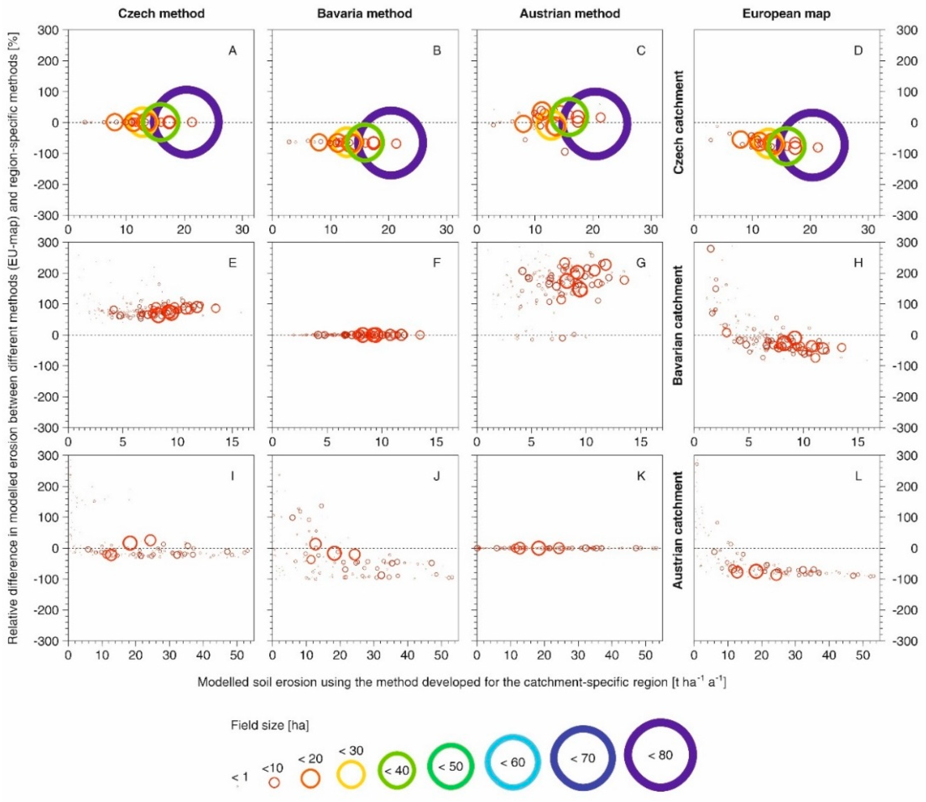
3.2. Distribution of National Differences

As shown in this comparison of the different national/regional implementations of the USLE, it is hardly possible to derive reasonable standardized soil conservation rules on a larger scale. This is especially problematic as the different methods do not simply lead to a bias of modelled erosion of all fields, but also change the catchment internal arrangement of fields with low to high erosion rates (Figure 4B,C,E,G,I,J). In BY and AT, the most pronounced differences between modelled field-specific erosion from different methods were found for small fields with low erosion, which regarding soil conservation is more or less unproblematic. However, in some cases, there seemed to be a tendency that the relative differences between methods increase with increasing erosion (> 5 t ha−1 a−1) (Figure 4B,E,G), which might lead to wrong decisions with respect to allocating soil conservation measures. In practice, this study underlines that soil erosion assessment, as well as erosion control, highly depends on the region or nation. There are very different approaches, requirements, and lists of soil control measures and technologies, which are applied within individual countries. The same methods of determination of the necessity of the implementation measures and critical values differ from country to country. While in Austria, farmers are required to follow GAEC (Good Agricultural and Environmental Conditions) standards to fulfil requirements of Cross Compliance policy, which do not include any soil erosion control measures, in CZ, eight standards of GAEC are implemented, where two of them deal with soil erosion control (and are based on the above-introduced methodology of soil erosion risk quantification). The list of measures applicable to fulfil requirements varies in time, according to political discussion of individual professional clusters within the agricultural chamber—i.e., removing stones is accepted as a soil erosion control measure within potato production to fulfil the GAEC 5 requirements in CZ. In BY, different initiatives exist using erosion modelling to encourage farmers to adopt soil conservation measures. These are mostly orientated towards the reduction of off-site effects and meet the targets of the Water Framework Directive [11]. The same is true concerning of determination of fields where measures are required to apply. Different approaches, input values, and detailed methodologies (as documented in previous paragraphs) are implemented at state level within the three countries compared within the paper. If standards were applied across borders, high inequity would be introduced for individual countries in the sense of what measures are required to be respected/implemented by individual farmers.
Furthermore, the process of seeking optimum methods and input data, updated tolerable soil losses, and critical values to determine soil conservation measures in individual countries is very dynamic. Since the beginning of 2020, for example, a new approach for soil erosion protection has been planned by the Ministry of Agriculture in CZ. In BY, the administration of the Bavarian State Research Centre for Agriculture is discussing the use of rainfall radar data to derive yearly and seasonal rainfall erosivity data in a 1 km × 1 km grid [54]. Last but not least, the AT results presented in this paper have to be considered as intermediate, since the computation methods of the LS and C factors were adapted from a periodic report of an ongoing project. Final results with revised LS and C factor computations have become available only after termination of this work [55]. The updated information demonstrates an overall reduction of erosion by approximately 20% but a similar spatial distribution of soil loss compared to the methodology used in this study.

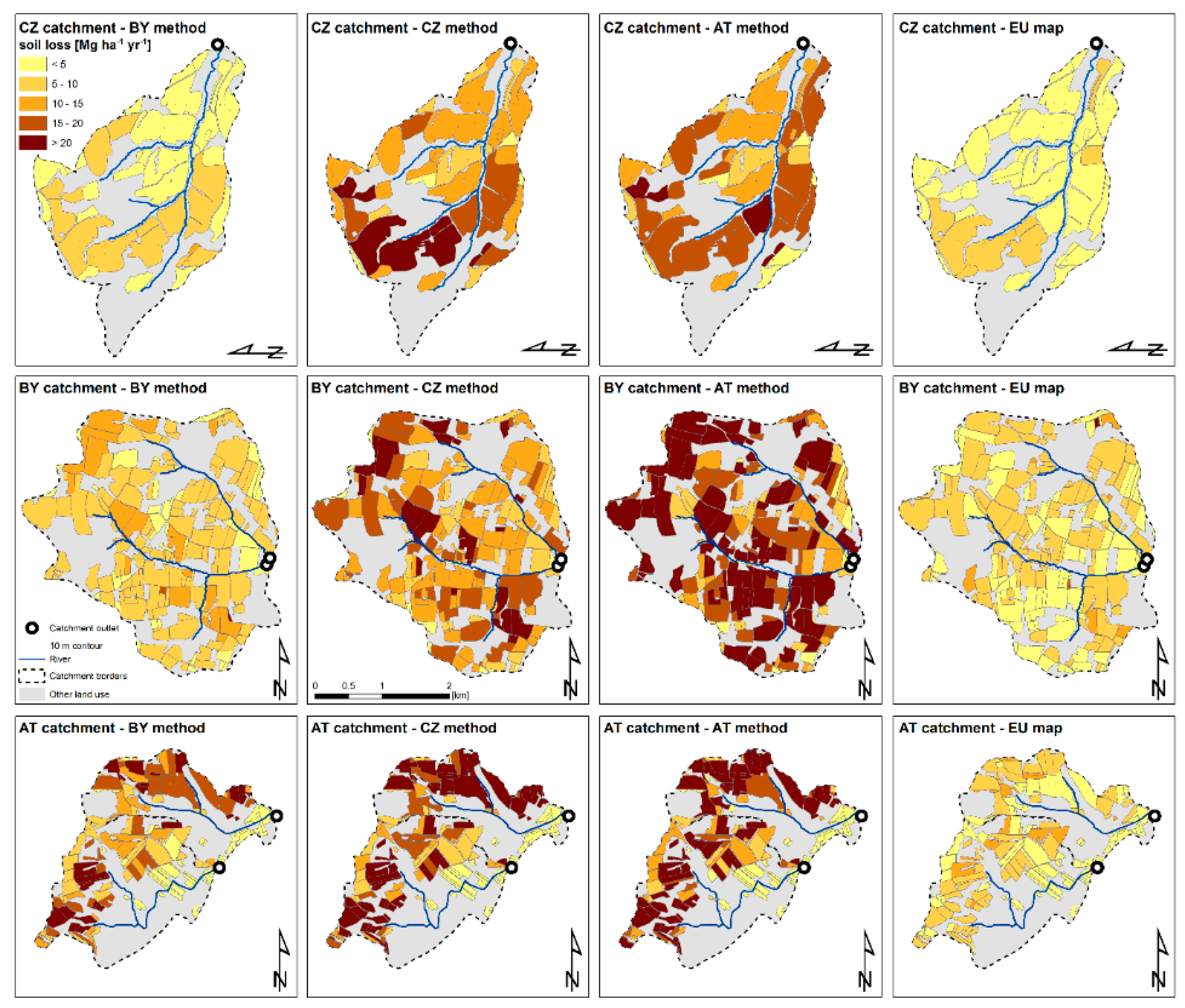
3.3. Comparison of National vs. European Soil Erosion Map

This dilemma of missing standardization and harmonization calls for a larger scale model application. Such a challenging approach was published by Panagos et al. [19] using an adapted version of the RUSLE and providing publicly available soil erosion information for the entire EU in a 100 m × 100 m grid (https://esdac.jrc.ec.europa.eu/content/soil-erosion-water-rusle2015). In general, the model results of this study showed higher mean erosion for all sites and applied model approaches. The differences were most pronounced between the European map and the AT and CZ approach (Figure 3; column on the right). A field-by-field comparison (Figure 4D,H,L) gives more insights into why the national/regional approaches differ substantially from the European map. At the site in Bavaria and Austria, which both are dominated by small fields (mean size: 3.1 ha and 2.2 ha, respectively), the European map overestimates the erosion on fields with little erosion while it underestimates the erosion on fields with substantial erosion (Figure 4D,H,L). Differences in erosion of individual fields results to a large extend from differences in LS factor. A raster cell size of 25 m × 25 m used to calculate the LS factor which is then aggregated into the 100 m × 100 m European map substantially smoothens the slope variability and hence must lead to an underestimation of steep and overestimation of flat slopes. This relation was shown in several earlier studies [56,57]. The effect is much smaller in the CZ test catchment as the mean field size of 11.6 ha is much larger and hence aggregating erosion to field means already results in an averaging of steep and flat areas within these fields. In consequence, the correlation between the CZ site modelled with the CZ method and the European map is much stronger (R2 = 0.30; p < 0.001) than at the BY and AT sites using the respective regional methods (R2 = 0.12 and 0.15; p< 0.001). The available input data for the European map is highly fragmented due to major national differences in data sources and data accuracies. For a homogenized pan-European soil erosion map, assumptions are required that include high uncertainties (e.g., [58]). Moreover, region-specific adaptations and optimizations of the USLE (see examples in methods) cannot be considered in a harmonized procedure for the entire EU.
However, apart from the scale issue, the European map shows generally much smaller erosion means as compared to the national/regional approaches (Figure 4D,H,L). For the Bavarian and the Czech site, the Panagos et al.’s [19] map shows a mean erosion of 5.64 and 4.17 ha−1 a−1, which is about 30% and 70% less erosion compared to the site-specific modelling. This would of course lead to much softer requirements to farmers to apply soil conservation techniques and measures in these catchments. Hence, there seems to be still a strong need for more cooperation and homogenization of data and methods to bridge the gap between national and EU-wide input data and methodologies.

4. Conclusions

In this study, three different USLE implementations, as used by environmental administrations in CZ, BY, and AT to assess agricultural erosion potential, were applied in three test catchments (7–10 km2) in CZ, BY, and AT. The results indicate that, even if all administrations use USLE technology, the regional model adaptations and implementation techniques result in substantial differences in test catchment specific mean erosion. Mean erosion of the three methods applied at all sites vary substantially (CZ: 10.4 ± 4.88 t ha−1 a−1; BY: 14.4 ± 6.47 t ha−1 a−1; AT: 16.7 ± 6.65 t ha−1 a−1). Much more pronounced differences were modelled for individual fields. The relative difference between methods was highest for small fields with little erosion (approx. < 2 t ha−1 a−1) which should be more or less unproblematic with respect to implementing potential soil conservation measures based on the modelling approaches. However, in some cases, differences in modelled field-specific erosion between methods increase for fields with increasing erosion (in CZ also in the case of larger fields). This indicates how sensitive conservation planning is to different USLE implementations, which usually gives farmers incentives only to the most erosion-prone fields in an area.
A comparison of the region-specific USLE approaches presented in this study with the revised USLE-base European erosion map developed by Panagos et al. [19] shows the problems and limitations of harmonization procedures. First, using a spatial resolution of 100 × 100 m2 for most USLE factors and aggregating higher resolution factors into an overall erosion potential on this grid size (as done on the European level [19]) obviously results in an erosion overestimation in case of fields with little erosion and an underestimation in case of fields with larger erosion. Second, the catchment-wide mean erosion from the European map underestimates the mean erosion compared to the region-specific USLE methods.
In general, the results indicate that even if a large proportion of countries within the EU use USLE technology to assess erosion potential as basis for soil conservation planning, a truly consistent method does not exist and more efforts are needed to homogenize the different methods without losing the specific USLE knowledge developed in the different regions over the last decades.

Author Contributions

Conceptualization: T.D. and P.F.; methodology, T.D., P.F., F.W., J.K., P.S. and E.S.; validation, T.D., P.F., F.W., J.K., P.S. and E.S.; formal analysis, T.D., P.F., F.W., J.K., P.S. and E.S.; data curation, F.W., J.K., and E.S.; writing—original draft preparation, P.F.; writing—review and editing, T.D., P.F., F.W., J.K., P.S. and E.S.; visualization, P.F. and F.W. project administration, T.D. and P.F.; funding acquisition, T.D. and P.F. All authors have read and agreed to the published version of the manuscript.

Funding

This research was funded by German Academic Exchange Service (DAAD), grant number 57393320, and the Ministry of Education, Youth, and Sports of the Czech Republic, grant number MOBILITY 8J20DE005 and 8J18DE006.

Acknowledgments

We specifically acknowledge the support through Melanie Treisch from the Bavarian State Research Centre for Agriculture (LfL Bayern).

Conflicts of Interest

The authors declare no conflict of interest. The funders had no role in the design of the study; in the collection, analyses, or interpretation of data; in the writing of the manuscript, or in the decision to publish the results.

References

  1. Montanarella, L.; Pennock, D.J.; McKenzie, N.; Badraoui, M.; Chude, V.; Baptista, I.; Mamo, T.; Yemefack, M.; Aulakh, M.S.; Yagi, K.; et al. World’s soils are under threat. SOIL 2016, 2, 79–82. [Google Scholar] [CrossRef] [Green Version]
  2. Pimentel, D. Soil erosion: A food and environmental threat. Environ. Dev. Sustain. 2006, 8, 119–137. [Google Scholar] [CrossRef]
  3. Pimentel, D.; Burgess, M. Soil erosion threatens food production. Agriculture 2013, 3, 443–463. [Google Scholar] [CrossRef] [Green Version]
  4. Stavi, I.; Lal, R. Loss of soil resources from water-eroded versus uneroded cropland sites under simulated rainfall. Soil Use Manag. 2011, 27, 69–76. [Google Scholar] [CrossRef]
  5. Su, Z.A.; Zhang, J.H.; Nie, X.J. Effect of soil erosion on soil properties and crop yields on slopes in the Sichuan basin, China. Pedosphere 2010, 20, 736–746. [Google Scholar] [CrossRef]
  6. Doetterl, S.; Berhe, A.A.; Nadeu, E.; Wang, Z.G.; Sommer, M.; Fiener, P. Erosion, deposition and soil carbon: A review of process-level controls, experimental tools and models to address C cycling in dynamic landscapes. Earth Sci. Rev. 2016, 154, 102–122. [Google Scholar] [CrossRef]
  7. Verstraeten, G.; Poesen, J.; Govers, G.; Steegen, A. The off-site impacts of soil erosion by water in central Belgium. Belgeo 2000, 1, 227–240. [Google Scholar]
  8. Krasa, J.; Dostal, T.; Van Rompaey, A.; Vaska, J.; Vrana, K. Reservoirs’ siltation measurments and sediment transport assessment in the Czech Republic, the Vrchlice catchment study. Catena 2005, 64, 348–362. [Google Scholar] [CrossRef]
  9. Good Agriculture and Environmental Condition: Web Database. Available online: https://marswiki.jrc.ec.europa.eu/gaec/appl.php (accessed on 19 March 2020).
  10. Council of the European Union; European Parliament. REGULATION (EU) 2017/2393 OF THE EUROPEAN PARLIAMENT AND OF THE COUNCIL (of 13 December 2017) Amending Regulations (EU) No 1305/2013 on Support for Rural Development by the European Agricultural Fund for Rural Development (EAFRD), (EU) No 1306/2013 on the Financing, Management and Monitoring of the Common Agricultural Policy, (EU) No 1307/2013 Establishing Rules For Direct Payments to Farmers under Support Schemes within the Framework of the Common Agricultural Policy, (EU) No 1308/2013 Establishing a Common Organisation of the Markets in Agricultural Products and (EU) No 652/2014 Laying down Provisions for the Management of Expenditure Relating to the food Chain, Animal Health and Animal Welfare, and Relating to Plant Health and Plant Reproductive Material; Commission, E., Ed.; The European Parliament: Brussels, Belgium, 2017. [Google Scholar]
  11. Anonymous. Directive 2000/60/EC of the European Parliament and of the Council of 23 October 2000 establishing a framework for Community action in the field of water policy. Off. J. 2000, 327, 1–73. [Google Scholar]
  12. Schwertmann, U.; Vogl, W.; Kainz, M. Bodenerosion Durch Wasser-Vorhersage Des Abtrags Und Bewertung Von Gegenmassnahmen; Ulmer Verlag: Stuttgart, Germany, 1987; p. 64. [Google Scholar]
  13. DIN 19708: Bodenbeschaffenheit - Ermittlung der Erosionsgefährdung von Böden durch Wasser mit Hilfe der ABAG. Soil Quality - Predicting Soil Erosion by Water by Means of ABAG; Beuth Verlag: Berlin, Germany, 2017.
  14. Schob, A.; Schmidt, J.; Tenholtern, R. Derivation of site-related measures to minimise soil erosion on the watershed scale in the Saxonian loess belt using the model EROSION 3D. Catena 2006, 68, 153–160. [Google Scholar] [CrossRef]
  15. Wischmeier, W.H.; Smith, D.D. A universal soil-loss equation to guide conservation farm planning. Int. Congr. Soil Sci. Trans. 1960, 7, 418–425. [Google Scholar]
  16. Wischmeier, W.H.; Smith, D.D. Predicting Rainfall Erosion Losses-A Guide to Conservation Planning; Print Office: Washington, DC, USA, 1978. [Google Scholar]
  17. Renard, K.G.; Foster, G.R.; Weesies, G.A.; Porter, J.P. RUSLE-Revised universal soil loss equation. J. Soil Water Conserv. 1991, 46, 30–33. [Google Scholar]
  18. Alewell, C.; Borrelli, P.; Meusburger, K.; Panagos, P. Using the USLE: Chances, challenges and limitations of soil erosion modelling. Int. Soil and Water Conserv. Res. 2019, 7, 203–225. [Google Scholar] [CrossRef]
  19. Panagos, P.; Borrellli, P.; Poesen, J.; Ballabio, C.; Lugato, E.; Meusburger, K.; Montanarella, L.; Alewell, C. The new assessment of soil loss by water in Europe. Environ. Sci. Policy 2015, 54, 438–447. [Google Scholar] [CrossRef]
  20. WRB, I.W.G. World Reference Base for Soil Resources 2006; FAO: Rome, Italy, 2006; pp. 1–145. [Google Scholar]
  21. Devátý, J.; Dostál, T.; Hösl, R.; Krása, J.; Strauss, P. Effects of historical land use and land pattern changes on soil erosion–Case studies from Lower Austria and Central Bohemia. Land Use Policy 2019, 82, 674–685. [Google Scholar] [CrossRef]
  22. Janeček, M.; Dostál, T.; Kozlovsky-Dufková, J.; Dumbrovský, M.; Hůla, J.; Kadlec, V.; Konečná, J.; Kovář, P.; Krása, J.; Kubátová, E.; et al. Protection of Agricultural Land from Erosion, in Czech (Ochrana Zemědělské Půdy Před Erozí), Certified Methodology for State Land Office; University of Life Sciences: Prague, Czech Republic, 2012. [Google Scholar]
  23. Brychta, J.; Janecek, M. Evaluation of discrepancies in spatial distribution of rainfall erosivity in the Czech Republic caused by different approaches using GIS and geostatistical tools. Soil Water Res. 2017, 12, 117–127. [Google Scholar] [CrossRef] [Green Version]
  24. Sauerborn, P. Die Erosivität der Niederschläge in Deutschland - Ein Beitrag Zur Quantitativen Prognose der Bodenerosion Durch Wasser in Mitteleuropa; Institut für Bodenkunde: Bonn, Germany, 1994; p. 189. [Google Scholar]
  25. DWD. Multi-Annual Grids of Precipitation Height over Germany 1981–2010; DWD: Offenbach, Germany, 2017. [Google Scholar]
  26. Strauss, P.; Klaghofer, E.; Blum, W.E.H.; Auerswald, K. Erosivität von Niederschlägen: Ein Vergleich Österreich - Bayern. Z. für Kult. und Landentwickl. 1995, 36, 304–308. [Google Scholar]
  27. Wagner, K. Neuabgrenzung Landwirtschaftlicher Produktionsgebiete in Österreich; Schriftenreihe der Bundesanstalt für Agrarwirtschaft: Vienna, Austria, 1990. [Google Scholar]
  28. Vopravil, J.; Janeček, M.; Tippl, M. Revised soil erodibility K-factor for soils in the Czech Republic. Soil Water Res. 2007, 2, 1–9. [Google Scholar] [CrossRef] [Green Version]
  29. Janeček, M.; Dostál, T.; Kozlovsky-Dufková, J.; Dumbrovský, M.; Hůla, J.; Kadlec, V.; Konečná, J.; Kovář, P.; Krása, J.; Kubátová, E.; et al. Ochrana Zemědělské Půdy Před Erozí (Erosion Conservation on Agricultural Land); The Czech University of Life Sciences: Prague, Czech Republic, 2012; pp. 1–113. [Google Scholar]
  30. Auerswald, K.; Fiener, P.; Martin, W.; Elhaus, D. Use and misuse of the K factor equation in soil erosion modeling: An alternative equation for determining USLE nomograph soil erodibility values. Catena 2014, 118, 220–225. [Google Scholar] [CrossRef]
  31. Auerswald, K.; Fiener, P.; Martin, W.; Elhaus, D. Use and misuse of the K factor equation in soil erosion modeling (vol 118, pg 220, 2014). Catena 2016, 139, 271. [Google Scholar] [CrossRef]
  32. Wischmeier, W.H.; Johnson, C.B.; Cross, B.V. A soil erodibility nomograph for farmland and construction sites. J. Soil Water Conserv. 1971, 26, 189–193. [Google Scholar]
  33. Strauss, P. Areal soil loss by water. In Hydrologischer Atlas Von Österreich; Bundesministerium für Land- und Forstwirtschaft, Umwelt und Wasserwirtschaft, Abteilung Wasserhaushalt: Vienna, Austria, 2007. [Google Scholar]
  34. Strauss, P.; Wolkerstorfer, G.; Buzas, K.; Kovacs, A.; Clement, A. Evaluated Model on Estimating Nutrient Flows Due to Erosion/Runoff in the Case Study Areas Selected; Deliverable 2.1-daNUbs project (EVK1-CT-2000-00051); Bundesamt für Wasserwirtschaft: Pentzenkirchen, Austria, 2005; p. 90. [Google Scholar]
  35. David, G.; Rafal, Z. Land Parcel Identification System (LPIS); Ministry of Agriculture of Czech Republic: Prague, Czech Republic, 2019. [Google Scholar]
  36. Desmet, P.J.J.; Govers, G. A GIS procedure for automatically calculating the USLE LS factor on topographically complex landscape units. J. Soil Water Conserv. 1996, 51, 427–433. [Google Scholar]
  37. Van Oost, K.; Govers, G.; Desmet, P. Evaluating the effects of changes in landscape structure on soil erosion by water and tillage. Landsc. Ecol. 2000, 15, 577–589. [Google Scholar] [CrossRef]
  38. McCool, D.K.; Foster, G.R.; Weesies, G.A. Slope Length and Steepness Factors (LS); Washington State University: Pullman, WA, USA, 1989; p. 41. [Google Scholar]
  39. McCool, D.K.; Brown, L.C.; Foster, G.R.; Mutchler, C.K.; Meyer, L.D. Revised slope steepness factor for the Universal Soil Loss Equation. Trans. Am. Soc. Agric. Eng. 1987, 30, 1387–1396. [Google Scholar] [CrossRef]
  40. Nearing, M.A. A single, continuous function for slope steepness influence on soil loss. Soil Sci. Soc. Am. J. 1997, 61, 917–919. [Google Scholar] [CrossRef]
  41. McCool, D.K.; Foster, G.R.; Weesies, G.A. Slope length and steepness factors (LS). In Predicting Soil Erosion by Water: A Guide to Conservation Planning with the Revised Universal Soil Loss Equation (RUSLE); Renard, K.G., Foster, G.R., Weesies, G.A., McCool, D.K., Yoder, D.C., Eds.; U.S. Department. Agriculture: Washington, WA, USA, 1997; pp. 101–141. [Google Scholar]
  42. Quinn, P.F.; Beven, K.; Chevallier, P.; Planchon, O. The prediction of hillslope flow paths for distributed hydrological modelling using digital terrain models. Hydrol. Process. 1991, 5, 59–79. [Google Scholar] [CrossRef]
  43. Protierozní Kalkulačka. Available online: https://kalkulacka.vumop.cz/ (accessed on 15 October 2019).
  44. Auerswald, K. Schätzung des C-Faktors aus Fruchtartenstatistiken für Ackerflächen in Gebieten mit subkontinentalem bis subatlantischem Klima nördlich der Alpen. Landnutz. und Landentwickl. 2002, 43, 269–273. [Google Scholar]
  45. Stenitzer, E.; Diestel, H.; Zenker, T.; Schwartengaber, R. Assessment of capillary rise from shallow groundwater by the simulation model SIMWASER using either estimated pedotransfer functions or measured hydraulic parameters. Water Resour. Manag. 2007, 21, 1567–1584. [Google Scholar] [CrossRef]
  46. Stenitzer, E. 2000: SIMWASER—Ein physikalisches Kompartimentmodell Zum Bodenwasserhaushalt. In und Klotz D (Herausgeber): Methoden der Sickerwassermodellierung - Theorie und Praxis, GSF-Bericht 18/2000; Seiler, K.P., Ed.; GSF - Forschungszentrum für Umwelt und Gesundheit GmbH: Neuherberg, Germany, 2000; pp. 29–34, ISSN 0942-6809. [Google Scholar]
  47. Renard, K.G.; Foster, G.R.; Weesies, G.A.; McCool, D.K.; Yoder, D.C. Predicting Soil Erosion by Water: A Guide to Conservation Planning with the Revised Universal Soil Loss Equation (RUSLE); USDA-ARS: Washington WA, USA, 1996. [Google Scholar]
  48. Fiener, P.; Wilken, F.; Auerswald, K. Filling the gap between plot and landscape scale—eight years of soil erosion monitoring in 14 adjacent watersheds under soil conservation at Scheyern, Southern Germany. Adv. Geosci. 2019, 48, 31–48. [Google Scholar] [CrossRef] [Green Version]
  49. Wilken, F.; Ketterer, M.; Koszinski, S.; Sommer, M.; Fiener, P. Unravel the role of water and tillage erosion in an intensively used agricultural landscape in north-eastern Germany based on 239+240Pu tracer measurements. SOIL Discuss. 2020. [Google Scholar] [CrossRef] [Green Version]
  50. Fiener, P.; Wilken, F.; Aldana-Jague, E.; Deumlich, D.; Gómez, J.A.; Guzmán, G.; Hardy, R.A.; Quinton, J.N.; Sommer, M.; Van Oost, K.; et al. Uncertainties in assessing tillage erosion – How appropriate are our measuring techniques? Geomorphology 2018, 304, 214–225. [Google Scholar] [CrossRef] [Green Version]
  51. Fischer, F.K.; Winterrath, T.; Auerswald, K. Temporal and spatial scale and positional effects on rain erosivity derived from point-scale and contiguous rain data. Hydrol. Earth Syst. Sci. Discuss. 2018. [Google Scholar] [CrossRef] [Green Version]
  52. Fiener, P.; Neuhaus, P.; Botschek, J. Long-term trends in rainfall erosivity - analysis of high resolution precipitation time series (1937-2007) from Western Germany. Agric. For. Meteorol. 2013, 171, 115–123. [Google Scholar] [CrossRef]
  53. Fischer, F.K.; Kistler, M.; Brandhuber, R.; Maier, H.; Treisch, M.; Auerswald, K. Validation of official erosion modelling based on high-resolution radar rain data by aerial photo erosion classification. Earth Surf. Process. Landf. 2018, 43, 187–194. [Google Scholar] [CrossRef]
  54. Fischer, F.; Hauck, J.; Brandhuber, R.; Weigl, E.; Maier, H.; Auerswald, K. Spatio-temporal variability of erosivity estimated from highly resolved and adjusted radar rain data (RADOLAN). Agric. For. Meteorol. 2016, 223, 72–80. [Google Scholar] [CrossRef]
  55. Strauss, P.; Schmaltz, E.; Krammer, C.; Zeiser, A.; Weinberger, C.; Kuderna, M.; Dersch, G. Bodenerosion in Österreich - Eine Nationale Berechnung Mit Regionalen Daten Und Lokaler Aussagekraft Für ÖPUL; The Federal Agency for Water Management: Petzenkirchen, Austria, 2020; p. 150. [Google Scholar]
  56. Auerswald, K.; Fiener, P.; Dikau, R. Rates of sheet and rill erosion in Germany-A meta-analysis. Geomorphology 2009, 111, 182–193. [Google Scholar] [CrossRef]
  57. Guth, P.L. Geomorphometry from SRTM: Comparision to NED. Photogramm. Eng. Remote Sens. 2006, 72, 269–277. [Google Scholar] [CrossRef]
  58. Auerswald, K.; Fiener, P.; Gomez, J.A.; Govers, G.; Quinton, J.; Strauss, P. Comment on “Rainfall erosivity in Europe” by Panagos et al. (Sci. Total Environ., 511, 801-814, 2015). Sci. Total Environ. 2015, 532, 849–852. [Google Scholar] [CrossRef]
Figure 1. Topography and land use of test catchments.
Applsci 10 03647 g001
Figure 2. Boxplots of variability in soil loss based on data aggregated to parcels/fields; boxes indicate median and 25% and 75% quantiles, while whiskers give 5% and 95% quantiles.
Applsci 10 03647 g002
Figure 3. Modelled mean erosion per parcel for the three test catchments in Czech Republic, Bavaria, and Austria using the different standard methods applied in the respective environmental administration. Moreover, the field means based on the EU map [19] are given in the right column.
Applsci 10 03647 g003
Figure 4. Relative difference between field erosion modelled with different methods (and EU map [19]) and the method potentially best representing the catchment (e.g., in the CZ catchment: Czech (A), Bavarian (B), Austrian methods (C), and European map (D) vs. CZ method). Each data point represents the mean soil loss of a field.
Applsci 10 03647 g004
Table 1. Test catchment characteristics including land management.
Test Catchments
UnitCZBYAT
Catchment properties
Latitude°49.7748.4148.16
Longitude°14.8312.7215.14
Elevation a.s.l.m433420255
Sizekm27.7510.17.32
Main slope°6.3 ± 3.96.7 ± 3.84.6 ± 3.9
Mean precipitationmm a−1739844764
Mean temperature°C7.78.29.0
Arable land properties within catchment
Mean slope°5.8 ± 2.36.1 ± 2.94.1 ± 2.5
Mean field sizeha11.6 ± 15.43.08 ± 3.432.19 ± 2.52
Dominant soil type-CambisolCambisolCambisol
Dominant soil texture-sandy loamloamloam
Proportion of arable land%65.959.247.5
Small grain (proportion under soil conservation)%
(%)
83.8 (16.1)53.1 (0)46.5 (0)
Row crops (proportion under soil conservation)%
(%)
13.0 (0)45.2 (18.0)45.6 (0)
Perennial crops%3.11.17.9
Table 2. Official datasets used by administration as well as source data to calculate the Universal Soil Loss Equation (USLE) factors.
USLE FactorsOfficially Use Dataset (Standard)Data Source to Derive Officially Used DatasetData Provider (Web-Site)
Test catchment CZ
RAdopted from state accepted map1 min resolution precipitation data for meteorological stations (period of recent 10 years)Czech Hydrometeorological Institute (http://portal.chmi.cz/?l=en)
KAdopted by direct conversionSoil bonity map of CZState Land Office (https://www.spucr.cz/)
LS (DEM)Calculated according to description in methods5 × 5 m2 based on LIDAR DEMCzech Institute of Geodesy and Cartography (https://www.cuzk.cz/en)
LS (Land use)Calculated according to description in methodsLPIS parcel data setMinistry of Agriculture (http://eagri.cz/public/web/en/mze/)
COfficial tool usedAverage crop rotation for 2016Czech Statistical Institute
PStandard for arable land 1.0
Test catchment BY
RMap of long-term mean R factors (1981–2010) for each municipalityLong-term annual precipitation (1981–2010) in 1 × 1 km2 rasterGerman weather service (https://opendata.dwd.de/climate_environment)
KMap of K factor of arable land based on polygons of Soil Bonity MapSoil Bonity map of GermanyBayerische Vermessungsverwalt. Bodenschätzung. (https://geoportal.bayern.de/geodatenonline)
LS (DEM)Calculated according to description in methods5 × 5 m2 based on LIDAR dataBayerisches Landesamt für Landwirtschaft (LfL Bayern)
LS (land use)Calculated according to description in methodsINVEKOS data setBayerische Vermessungsverwalt. Flurstückskarten Bayern. (https://geoportal.bayern.de/geodatenonline)
CCalculated according to description in methodsProportion of row corps (with and without mulching), small grains and perennial crops within the catchment for the year 2016LfL Bayern
PStandard for arable land 0.85LfL Bayern
Test catchment AU
RCalculated according to description in methodsLong-term annual precipitation (1995–2015) in 1 × 1 km2 rasterFederal Ministry for Sustainability and Tourism, www.ehyd.gv.at; Zentralanstalt für Meteorologie und Geodynamik, www.zamg.ac.at
KMap of K factor of arable land based on polygons of Austrian soil classification mapAustrian soil classification mapAustrian Research Centre for Forests, https://bodenkarte.at/
LS (DEM)Calculated according to Description in methods10 × 10 m based on LIDAR dataMinistry for Sustainability and Tourism
LS (land use)Calculated according to Description in methodsINVEKOS data setMinistry for Sustainability and Tourism
CCalculated according to Description in methodsINVEKOS data setMinistry for Sustainability and Tourism
PStandard for arable land 1.0
Table 3. USLE factors and mean annual erosion calculated from individual raster cells at the different test catchments in the Czech Republic (CZ), Germany Bavaria (BY), and Republic of Austria (AT) according to the different standard methods used in all three regions.
CZ MethodBY MethodAT Method
USLE Factor/Mean ErosionUnitMean Arable LandSD 1Spatially DistributedMean Arable LandSD 1Spatially DistributedMean Arable Land SD 1Spatially Distributed
CZ Test Catchment
RN h−147.40.34yes59.8-no67.3 -no
Kt h ha−1 N−10.290.09yes0.290.09CZ data0.290.09CZ data
LS-3.792.82yes3.452.25yes3.762.72yes
C-0.27-no0.10-no0.210.05yes
P-1.00-no0.85-no1.00-no
At ha−1 a−114.411.8 4.953.72yes11.86.03yes
BY Test Catchment
RN h−145.7-yes72.90.27yes85.2-no
Kt h ha−1 N−10.450.06BY data0.450.06BY data0.450.06BY data
LS-2.472.15yes2.241.71yes2.351.99yes
C-0.28-no0.13-no0.230.05yes
P-1.00-no0.85-no1.00-no
At ha−1 a−114.312.1yes7.965.93yes20.917.5yes
AT Test Catchment
RN h−157.6- 61.9-no81.71.54yes
Kt h ha−1 N−10.480.14AT data0.480.14AT data0.480.14AT data
LS-2.312.34yes2.141.98yes2.282.23yes
C-0.30-no0.23-no0.210.07yes
P-1.00-no0.85-no1.00-no
At ha−1 a−119.419.92yes9.087.91yes21.524.6yes
1 SD is standard deviation.

