Organic Molecular Marker from Regional Biomass Burning—Direct Application to Source Apportionment Model

Abstract

To reduce fine particulate matter (PM_2.5) level, the sources of PM_2.5 in terms of the composition thereof needs to be identified. In this study, the experimental burning of ten types of biomass that are typically used in Republic of Korea, collected at the regional area were to investigate the indicated organic speciation and the results obtained therefrom were applied to the chemical mass balance (CMB) model for the study area. As a result, the organic molecular markers for the biomass burning were identified as they were varying according to chemical speciation of woods and herbaceous plants and depending upon the hard- and soft characteristics of specimens. Based on the source profile from biomass burning, major sources of PM_2.5 in the study area of the present study appeared as sources of biomass burning, the secondary ions, secondary particulate matters, which is including long-distance transport, wherein the three sources occupied most over 84% of entire PM_2.5. In regard to the subject area distinguished into residential area and on roads, the portion of the biomass burning appeared higher in residential area than on roads, whereas the generation from vehicles of gasoline engine and burning of meats in restaurants, etc. appeared higher on roads comparing to the residential area.

1. Introduction

One of the health risk factors, air pollution, has brought about approximately 3.7 million premature deaths in 2012, and is estimated to be affecting mostly on the mortality due to environmental effects by 2050 [1,2]. PM_2.5, one of the air pollutants, is a particulate of aerodynamic diameter less than 2.5 μm occupying 96% of those found in human lungs [3]. PM_2.5 penetrates the gas exchange region of the lungs and enters the circulatory system via passing through the respiratory barrier thereby spreads over the human body [4,5,6]. The Guidelines of Air Quality Management of World Health Organization recommend the employment of PM_2.5 instead of PM₁₀ as an indicator identifying air pollution; the public interest in the risk of PM_2.5 was increasing thereby [1].

To reduce the amount of PM_2.5, the sources of PM_2.5 in terms of the composition thereof needs to be identified. Depending on the sources of PM_2.5, the attribute of PM_2.5 can be distinguished into the artificial- and natural sources by which it can be divided into the primary matter directly discharged from sources and the secondary matter to be produced by chemical reaction of gas phase materials according to the photochemical reaction. The components of PM_2.5 consist mainly of carbons, such as organic mass (OM) including organic carbon (OC) and elemental carbon (EC), heavy metals and water soluble ions, etc. [7,8,9]. Less than 30% of organic compounds among the components can be identified as individual organic species wherein the part of materials of organic species exhibit very high source specificity [10]. These substances can be exploited as molecular markers to estimate the contribution of each source which are assigned in the model devised to identify sources of PM_2.5 [11,12]. Representative molecular markers comprise levoglucosan (pyrolysis of biomass), hopanes and steranes (combustion of fossil fuels) and cholesterol (combustion of meats) [10,12,13]. In South Korea, although use of biomass materials, such as pine trees, as the fuel of boilers has been growing in rural areas, in which farmers use vinyl greenhouses to raise fruits, vegetables and tropical plants during winter. However, the major source of serious air pollution problems in rural and neighboring urban areas is the natural forest fire during wintertime in the dry condition. The other source of air pollution due to biomass burning is the open-burning of agricultural crop residues after harvest to prepare the next cultivation even though the government prohibited the burning activities. As discussed above, the chemical properties of organic aerosol particles from biomass burning emissions vary significantly depending on the burning phase and biomass type. It is still a major challenge to investigate the chemical properties.

Distinguished sources of air pollutants can be employed as basic data for the reduction of emission of sources of air pollutants by which the contribution of air pollutants can be reduced. In general, diverse kinds of acceptance model techniques are used for the distribution of sources of air pollutants. Representative models for the distribution of sources of air pollutants comprise the principal component analysis (PCA), enrichment factors (EFs), chemical mass balance (CMB), positive matrix factorization (PMF), empirical orthogonal functions (EOF), multiple regression, Fourier transformation time series and other multivariate analysis, etc. [13,14,15,16,17,18,19,20,21,22,23]. Among them, the CMB model is most widely used to identify sources of PM_2.5 [24]. However, the CMB model accompanies uncertainties originated from errors for arbitrary measurements or errors of input variables (organic molecular markers) beyond analytic results and inputted molecular markers. Thus, component analysis of PM_2.5 and accuracy of input variables are needed for the CMB model [25].

The present study intends for the identification of sources of creation of PM_2.5 by employing the CMB model. For which, the 160 kinds of chemical components, comprising EC, OC, water soluble organic carbon (WSOC), water insoluble organic carbon (WIOC) and water soluble ions, etc. were analyzed after collecting PM_2.5 from the subject area of the present study. In addition, the experiments of burning of 10 kinds of biomass were carried out to secure accuracy of CMB model, and the results obtained therefrom were applied to the CMB model. The results obtained from the present study are expected to be employed as basic data for the distribution of sources of PM_2.5.

2. Materials and Methods

A biomass burning chamber consists of three parts (i.e., a combustion chamber (0.54 m³), primary dilution chamber (3.75 m³) and secondary dilution chamber (0.04 m³)). It was employed for generation of forest tree types (6) and agricultural crop residues (4) (Figure 1 and

Table 1. Research materials used in biomass burning.

Forest tree Types		Agricultural Crop Residues
		(Herbaceous Plants)
Item	Academic Name	Item	Academic Name
Pine needles	Pinus densiflora	Rice straw	Oryza sativa
Pine stem
Ginkgo leaves	Ginkgo biloba L.	Red pepper stem	Capsicum annuum
Maple leaves	Acer palmatum
Cherry leaves	Prunus serrulata var. spontanea	Soybean stem	glycine max
Cherry stem		Green perilla stem	Perilla frutescens var. japonica Hara

), which were sampled from rural and regional forest areas in Korea. Zero air was supplied into the combustion chamber using a mass flow controller. About 25 g of biomass for each combustion was loaded on the grid of the combustion stove. The smoke was drawn into a primary (3.75 m³) dilution chamber (1:1), followed by a secondary dilution chamber (0.04 m³) (1:10). PM_2.5 samples were collected on pre-baked 90-mm quartz-fiber filters, 47-mm quartz-fiber filters and 47-mm Teflon filters (Pall Gellman, Ann Arbor, MI, USA) using 92 L per minute (lpm) medium-volume sampler and a set of low volume samplers, respectively. The detailed operation conditions can be found at the previous publication [26].

2.1. Organic Speciation

For the determination of organic molecular markers, the quartz filter sample was extracted by sonication using dichloromethane for non-polar organic compounds (i.e., Polyaromatic hydrocarbons (PAHs), n-alkanes, cycloalkanes and steranes and hopanes) analyzed using gas chromatography-mass spectrometry (GC-MS) and methanol or purified water for polar organic compounds (i.e., levoglucosan, amino acids, resin acids, alkanoic acids, aromatic diacids and alkane dioic acids) quantified using liquid chromatography -tandem mass spectrometry (LC-MSMS). All data were blank corrected using field blank data. For each nonpolar organic sample, the final volume was adjusted to 500 μL to match the volume of the internal standard (samples and blanks were spiked with internal standards). Underivatized polar organic compounds were analyzed using LC-MSMS with internal standards (e.g., phthalic acid (D4)), the milli-Q water of 5.0 mL (or methanol some polar organic compounds (e.g., phthalates and cholesterol, etc.) was sonicated into the sample tube for the final extract volume. Hydrophilic interaction LC used an Eclipse XDB-C18 4.6-mm ID × 150 mm (5 mm) column as stationary phase with 10-mM ammonium acetate and acetonitrile in milli-Q water. Polar organic compounds was analyzed in multiple reaction monitoring application for the separation and detection of underivatized compounds. Regression coefficients of determination for seven point calibrations were from higher than 0.998. Absolute method of detection limits were in the range of 1.0–4.6 pg/m³. For all polar organic compounds, the final mass fragment transitions of quantification application such as fragmentor voltage, collision energy, quantifier and qualifier ions, were determined. The detailed analytical condition can be found at the previous study [27,28,29]

2.2. Analysis of Organic Carbon (OC) and Elemental Carbon (EC)

The OC/EC analysis used in this study used thermal-optical transmittance according to the National Institute of Occupational Safety and Health (NIOSH5040) protocol. The NIOSH5040 protocol consists of three major stages. At the first stage, the sample was heated to 870 °C with He gas, and the second stage it was heated to 870 °C in the presence of O₂. In the final third step, OC and EC were quantified using an internal standard (5% CH₄ in He) for each sample. In the assay process, 2 μg C /μL sucrose (monosaccharide, C₁₂H₂₂O₁₁) was used as external reference material for test and calibration of the equipment condition and quantification. The OC/EC classification of the NIOSH5040 protocol was determined to be the point at which the transmittance of the laser back to the initial transmittance after gradual decrease when it passed through the filter [30].

2.3. Analysis of Water Soluble Total Organic Carbon (WSOC) and Ion Components

The extract was analyzed by total organic carbon (TOC) analyzer to analyze the water soluble total organic carbon (WSOC) of the sample. As with OC, the contamination level and condition of the equipment were checked using the external standard substance of WSOC, 3-mg/L sucrose. The analysis conditions were as follows: 15% (NH₄)₂S₂O₈ and 6-M H₃PO₄ were used as the oxidizing agent and the buffer solution, respectively, and analyzed by mixing them at the flow rates of 0.50 μL/min and 2.00 μL/min, respectively. Additionally, Inorganic Carbon Remover (ICR) was used to prevent interference with inorganic carbon. The extract was analyzed, and ion components were detected. Ionic compounds were analyzed using ion chromatography (Metrohm 883 Switzerland). For the cation, a Metrohm Metrosep C₄ 250/4.0 column was used. As the eluent, 5-mM HNO₃ at a flow rate of 0.60 mL/min was used. For anions, a Metrohm Metrosep A Supp 5 150/4.0 column was used. As the eluent, 3.20-mM Na₂CO₃ and 1.00-mM NaHCO₃ were mixed. The flow rate was 0.70 mL/min and H₂SO₄ (50 mM) suppressor was used. The amount of sample injected for anion and cation analysis was 250 μL each [30,31].

2.4. Ambient PM_2.5 Sampling

Two sites (i.e., residential and roadside site) were simultaneously operated to collect 24-integrated PM_2.5 samples from May 9 to 13 (spring), August 4 to 8 (summer), October 11 to 13 (fall) in 2016 and January 8 to 10 in 2017 (winter). PM_2.5 samples were collected using the same as samplers in the biomass burning chamber for each site. Samples were shipped and stored frozen until analysis. The residential site is located on the campus of the Gwangju Institute of Science and Technology (GIST) (35°13′41.1” N and 126°50′36.3” E) in Korea. The site is situated about 8 km from the city center and is surrounded by agricultural, residential and commercial areas. Road site (35°18′21.1” N and 126°88′86.3” E) is closely located at the main road with heavy traffic surrounded by several businesses and restaurants and is also close to a main highway.

2.5. Source Apportionment Methods

The CMB model (EPA-CMB8.2) was applied to the results obtained during the intensive sampling campaign [32,33]. The CMB develops a solution based on a linear summation of products at a receptor location based on the abundance of source profiles and source contributions. The CMB model attempts to fit ambient speciated results from residential and roadside sites to a specified group of sources with corresponding molecular markers. In this study, uncertainties for CMB in molecular marker data points were defined as the maximum of two functions of spike recoveries, detection limits, and load blank standard deviations. The source profiles used in the study except the biomass burning is the profiles in the previous study [28]. The detailed CMB method can be found elsewhere [28].

3. Results and Discussion

3.1. Source Profile of Biomass Burning

Table 2. Distribution of chemical abundances in fine particulate matter (PM_2.5) mass.

Unit: μg/m3	Forest Tree Types						Agricultural Crop Residues
	Pine Needles	Pine Stem	Ginkgo Leaves	Maple Leaves	Cherry Leaves	Cherry Stem	Rice Straw	Soybean Stem	Green Perilla Stem	Red Pepper Stem
PM2.5	99,816	78,438	102,111	118,201	86,759	43,808	77,252	107,997	69,945	40,805
OC	53,514	28,566	53,794	60,307	49,993	14,457	41,548	55,554	27,886	11,602
EC	6496	8587	2673	2886	7446	2649	1392	5485	10,584	4719
Ions	4861	4219	5116	3369	7004	4890	2756	5527	9586	7029
Class-OC
WIOC	19,785	2284	30,458	30,882	20,519	1678	9482	13,139	1764	725
WSOC	33,728	26,281	23,335	29,425	29,474	12,779	32,066	42,415	26,121	10,877
Class-WIOC
PAHs	1179	653	134	172	191	201	170	183	426	105
Alkanes	291	102	969	1006	729	302	797	697	167	128
Class-WSOC
alkanoic acids	6311	2750	7424	4848	3593	1252	6644	5986	1006	570
benzene carboxylic acid	14	19	16	26	18	8	0	31	30	10
Di- Carboxylic acid	352	124	80	137	94	62	196	230	32	19
Amino acids	32	10	28	37	8	11	81	67	11	11
levoglucosan	1751	1950	1452	1783	2043	2274	1499	1656	1747	1308
Class-Ions
Potassium	660	1326	2004	507	3298	1830	626	1382	4433	3424
Sulfate	2040	1356	1436	1312	1488	1230	1152	1682	2996	1742
Nitrate	1680	964	957	1014	1138	960	701	1682	1797	931
Ammonium	480	573	718	537	1080	870	276	781	359	931

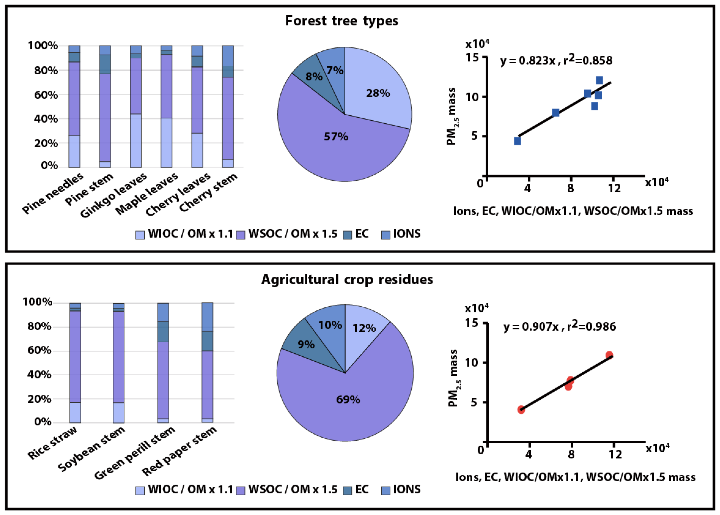
and Figure 2 show the emission in chemical classes of PM_2.5 from burning of woods and agricultural byproducts. The burning materials appeared according to characteristics thereof; approximately 48%, 7% and 6% of chemical components that consist of PM_2.5 appeared as OC, ionic compounds and EC, respectively. Based on results of previously conducted studies, approximately 49% of chemical components except for OC, EC and ionic chemical components, are estimated to be comprised of heavy metals, tiny amount of moisture, H, N, S and O, etc. that consist of organic substances other than carbon components [7,8,9].

To estimate the contents of H, N, S and O except for carbon components, the ratios of OM/OC, based on molecular weight of 114 individual OC compounds which were analyzed in the present study, were calculated. From calculations of OM/OC, the WIOC appeared as 1.1 while the WSOC appeared as 1.5. Approximately 66% of chemical components consisting of PM_2.5 appeared as OC based organic matters from the application of the ratio of OM/OC to calculations of WIOC and WSOC, while the occupancy of components of OC, EC and ionic chemical components in PM_2.5 appeared as 79%. The correlation of the ratio of OM/OC with PM_2.5 was identified wherein the correlation coefficient more than 0.85 was found thereby the estimation of chemical components consisting of PM_2.5 through employing the ratio of OM/OC was identified reliable as shown in Figure 2.

As a means to appraise the source of emission of PM_2.5, the ratio of OC/EC is used [34]. The ratio of OC/EC of PM_2.5 resulted from the burning of coal has been known to be distributing in the range 1.6–3 [35,36] while the ratio of OC/EC of PM_2.5 resulted from combustion of engine has been known to be distributing in the range 0.5–1.3 [16,37]. The ratio of OC/EC of PM_2.5 emitted from the biomass burning has been known over 3 which is higher than those of other sources; according to part of previously conducted studies, the ratio of OC/EC appeared higher than 12 of rice straw and 24 of wheat straw [37,38]. The ratio of OC/EC resulted from the biomass burning appeared distributing in the range 2.46–29.85 wherein the mean ratio thereof was 10.98. The ratio of OC/EC of 8 specimens among 10 specimens of analysis appeared over 3.0 and corresponded to results of previous studies however the ratios of OC/EC of stems of red-pepper and green perilla appeared below 3.0 suggesting different consequences from results of previous studies. To identify the causes behind the consequences, the specimens were distinguished into the hard ones of higher density (pine trees, cherry tree, red-pepper stems and stems of green perilla) and soft ones of lower density (pine needles, gingko leaves, maple leaves, cherry leaves, rice straws and stems of beans). The resulting ratio of 15.99 of OC/EC of soft specimens appeared relatively high while the ratio of 3.47 of OC/EC of hard specimens appeared lower than that of soft specimens.

The four chemical components of K⁺, SO₄²⁻, NO₃⁻ and NH₄⁺, constituting PM_2.5, were analyzed as ionic components. Contents of respective components of PM_2.5 appeared as approximately 2.36% of K⁺, 1.99% of SO₄²⁻, 1.43% of NO₃⁻ and 0.8% of NH₄⁺. Among them, K⁺ has been known as a major indicator ingredient of biomass burning; the level of content of K⁺ contained in dried woods has been known approximately over 0.1%, over 0.2% for dried herbaceous plant and over 3% for crops such as olive, etc. [39]. The K⁺, contained in crops, is emitted as KCl, KOH or K⁺ at temperature over 1000 K [40] and according to previously conducted studies, the K⁺ in PM_2.5, discharged from biomass burning, has been known to be contained 1%–10% in wheat straw and stems of maize and over 10% in rice straws [41]. The content of K⁺ analyzed in the present study appeared with lower levels of average 1.82% in the six woods and average 3.33% in herbaceous plants comparing to results reported from previous studies. In particular, the specimens of rice straw, analyzed in the present study, contained approximately 0.81% of K⁺ showing significant difference from results of previous studies.

Generally, in the case of using K⁺ as an indicator material of the biomass burning, the ratio of K⁺/EC is used [41].

Table 3. Ratios of K⁺/elemental carbon (EC) for crop residue emissions from this study compared to similar measurements reported elsewhere.

Type of Biomass	Measurement Approach	PM Size	K+/EC	References
Wood (pine needles)	chamber	PM2.5	0.10	this study
Wood (pine stem)	chamber	PM2.5	0.15	this study
Wood (ginkgo leaves)	chamber	PM2.5	0.75	this study
Wood (maple leaves)	chamber	PM2.5	0.18	this study
Wood (cherry leaves)	chamber	PM2.5	0.44	this study
Wood (cherry stem)	chamber	PM2.5	0.69	this study
Rice straw	chamber	PM2.5	0.45	this study
Soybean stem	chamber	PM2.5	0.25	this study
Green perilla stem	chamber	PM2.5	0.42	this study
Red pepper stem	chamber	PM2.5	0.73	this study
Wheat straw	chamber	PM2.5	2.26	Ni et al. 2017
Rice straw	chamber	PM2.5	3.45	Ni et al. 2017
Corn stalk	chamber	PM2.5	1.12	Ni et al. 2017
Wheat straw	chamber	PM2.5	2.2	Hays et al. 2005
Wood (Pine)	wind tunnel	PM10	0.19	Turn et al. 1997
Wood (Pine)	field measurement	PM2.5	0.76	Zhang et al. 2012

shows the ratio of K⁺/EC derived from the previously conducted studies and from the present study. As presented in the table, the ratio of K⁺/EC of herbaceous plant, employed for the present study, appeared distributing in the lower range 0.25–0.73 comparing to the ratio of K⁺/EC of 1.12–3.45 of herbaceous plant employed for the previous studies. In particular, the ratio of K⁺/EC of rice straw, which was predicted as pseudo-crop, was 3.45 in the previous studies exhibiting significant difference from 0.45 of the present study. On the contrary, the ratio of K⁺/EC of woods of the present study appeared distributing in the range 0.1–0.75 which were similar to those of 0.19 and 0.76 of previously conducted studies. The similarity (of woods) and difference (of herbaceous plant) in the ratio of K⁺/EC of the present study from those of previously conducted studies were attributed to the differences in components of specimens, species and corresponding cultivation environment. In the present study, the leaves and branches of the part of specimens of woods were distinguished wherein the ratio of K⁺/EC in branches of pine tree and cherry tree appeared approximately 50% higher than those in the leaves thereof. This suggests the ratio of K⁺/EC can be varied according to the ratio of composition of leaves and branches to be burnt, though they belong to the same kind of biomass of identical species. In addition, the content of K⁺ in leaves and branches of cherry tree appeared higher than other woods with respective values of 3.80% and 4.18%, while the content of K⁺ in stems of green perilla and red-pepper appeared 6.34% and 8.39%, respectively, suggesting the contents of K⁺ appeared distributing in the variable range of 0.43%–8.39% according to species of crops. Additionally, the K⁺, contained in plants, is affected by microorganisms and amount of potassium in soil. Potassium is the one of major nutrients for the growth of plants, the representative element of fertilizer. Water soluble potassium among fertilizer elements spread over soils are absorbed by crops, whereas the solidified potassium are absorbed by crops via microorganisms enabling the solubilization of potassium [42]. Therefore, the amount of potassium, contained in plants, is significantly dependent on the cultivation environment of plants. In the meantime, the red-pepper in Korea is regarded as one of the crops creating the highest value added as well as essential seasoning agent for which the area of cultivation of 32,865 ha in 2018 for red-pepper appeared higher than that of other flavor vegetables [43]. In addition, since the red-peppers are cultivated in an open field, it is included as the representative one of burning of agricultural byproducts in the registry of national atmospheric pollutants in Korea. Based on these facts, the kinds of species and cultivation environment of crops in each country, and the emission of K⁺ from respective crops need to be identified preemptively for the employment of K⁺ as an indicator material of the biomass burning. This is because the crops to be cultivated in countries are different according to respective dietary habits and the emission of K⁺ varies significantly according to types of species of crops cultivated.

The OC, occupying the highest portion among the components of PM_2.5, was classified into WIOC and WSOC, wherein the ratio of WIOC to WSOC appeared as approximately 1.2; the occupancies of WIOC and WSOC in PM_2.5 were approximately 16% and 32%, respectively. 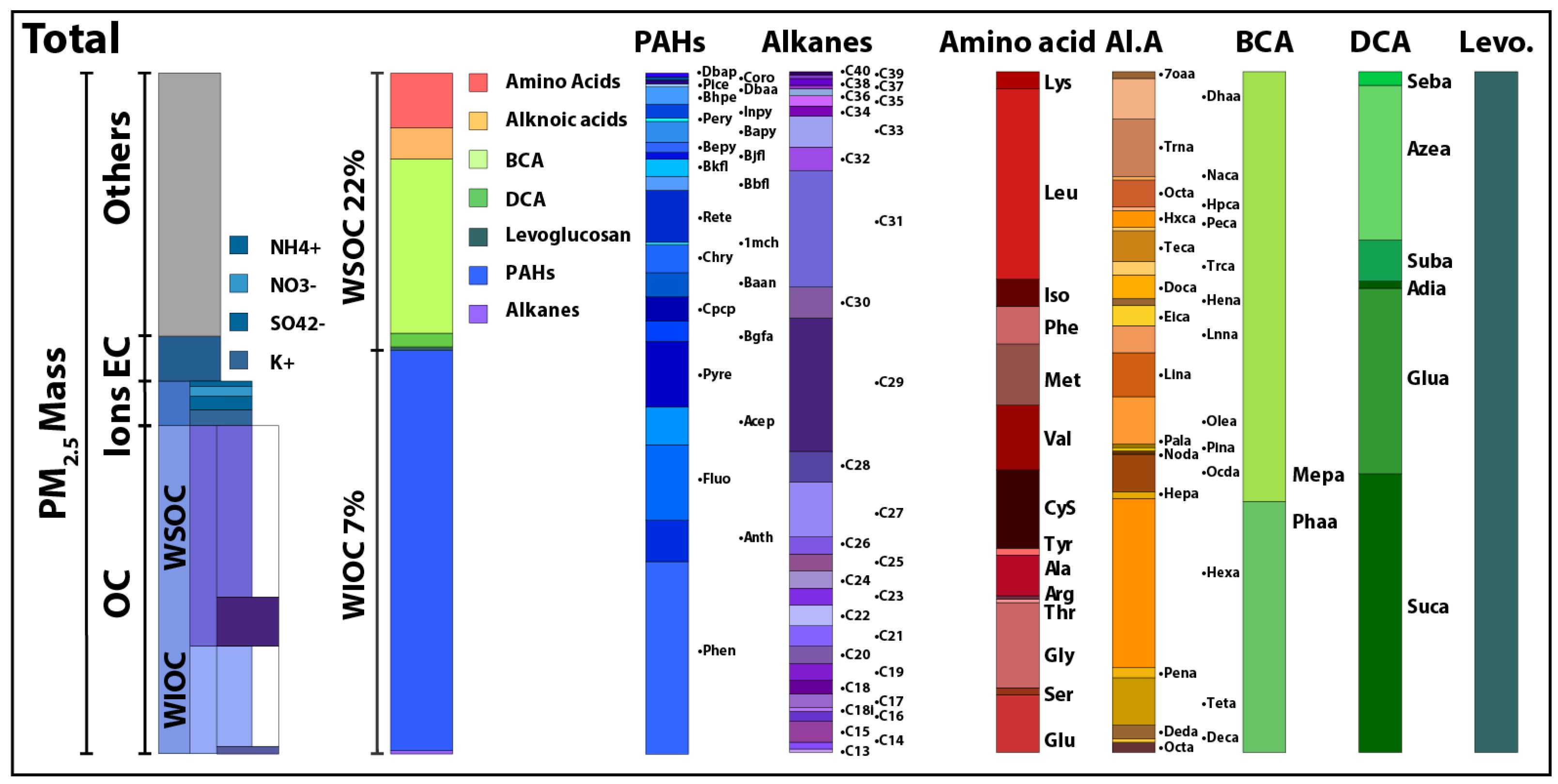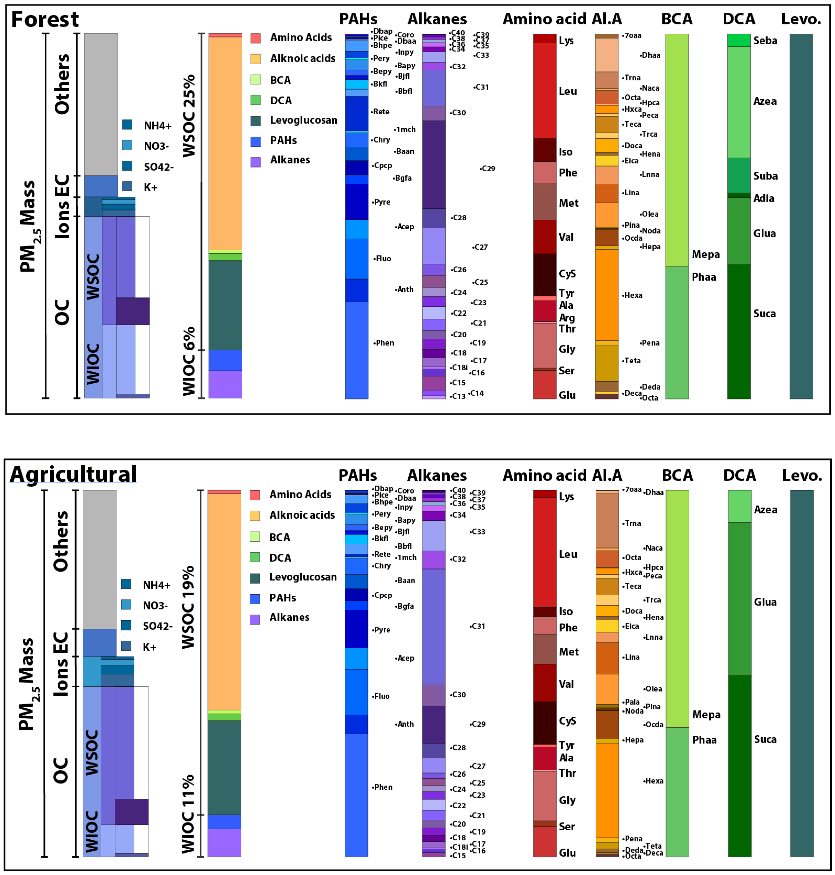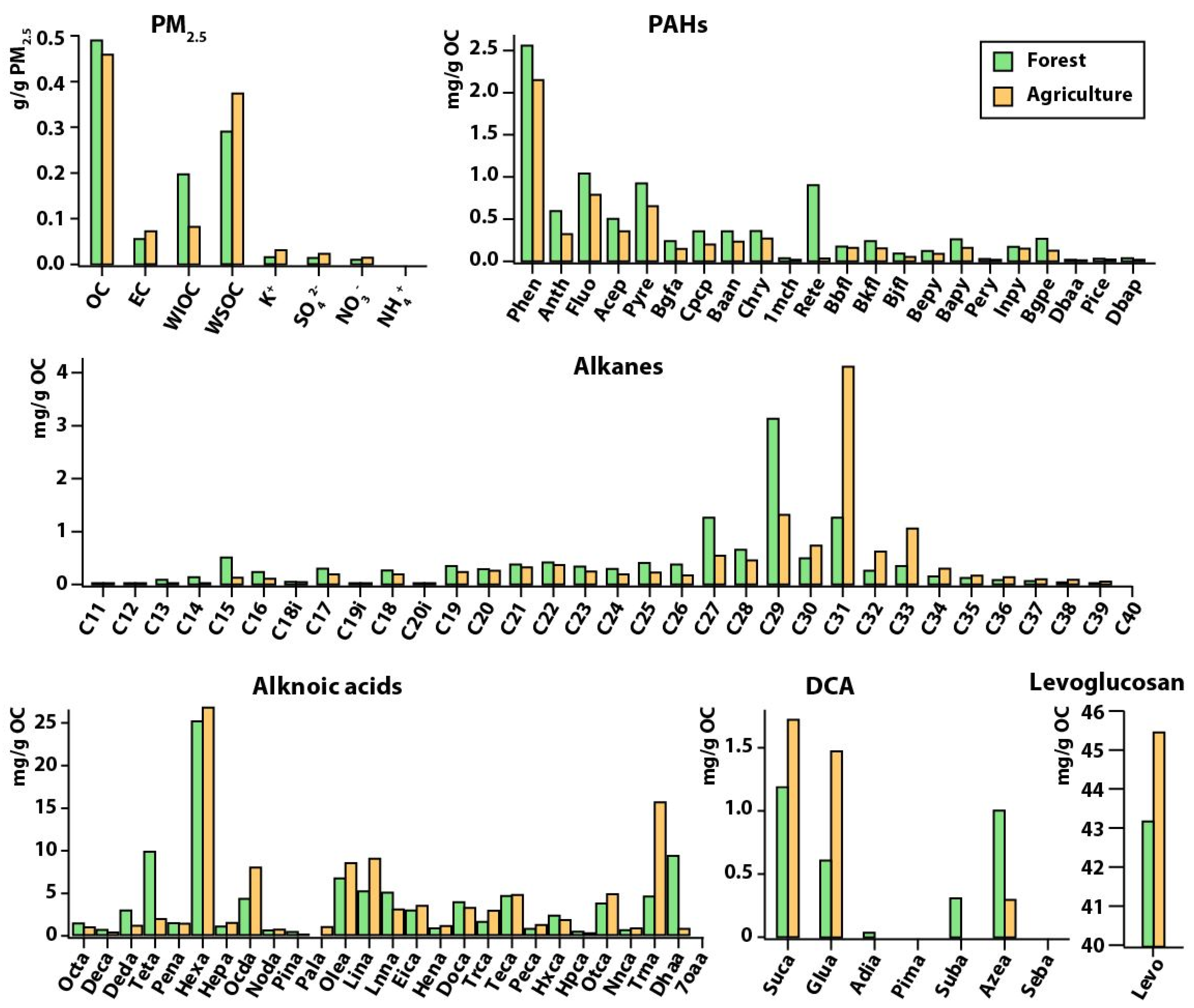Further, for the specimens of woods, the weight percentage of WIOC and WSOC to total weight of PM_2.5 appeared approximately 20.0% and 29.2%, respectively, whereas the weight percentage of WIOC and WSOC to total weight of PM_2.5 in herbaceous plant appeared approximately 8.5% and 37.6%, respectively. That is, the WIOC appeared higher in woods than in herbaceous plant, whereas the WSOC appeared higher in herbaceous plant than in woods. To determine the concentration of components in WIOC and WSOC, the 114 organic compounds, comprising the 23 compounds of PAHs and 33 compounds of alkanes were analyzed for the analysis of WIOC, as well as the 27 compounds of alkanoic acids, 8 compounds of benzene carboxylic acid, 7 compounds of di-carboxylic acid, 15 compounds of amino acids and levoglucosan, were analyzed for the analysis of WSOC. The results of the analysis are presented in Figure 3 and Figure 4. A total of 56 compounds of analysis of the PAHs and alkanes occupied approximately 7% of entire WIOC, wherein the weight percentage of PAHs and alkanes were 0.47% and 0.64%, respectively, to the weight of PM_2.5. PAHs appeared as in the order of phenanthrene > fluoranthene > pyrene; the emission of PAHs from woods appeared higher comparing to that from the herbaceous plant. In particular, retene was detected from the 3 ones among the 4 herbaceous plants with corresponding average concentration of 0.07 mg/g-OC, whereas the wood was detected from all 8 crops with corresponding average concentration of 0.92 mg/g-OC, which was higher than that of the herbaceous plant. In particular, retene, which is emitted from woods, was discharged highly from specimens of pine tree wherein the concentration in pine needle and in stalk exhibited 1.07 mg/g-OC and 6.11 mg/g-OC, respectively. For the case of alkanes, the detected ratios from woods and herbaceous plants appeared varying according to compounds of analysis. In the analyses from C₁₁ to C₂₉, the concentrations of wood exhibited higher emission than concentrations of herbaceous plant, whereas in the analyses from C₃₀ to C₄₀, the concentrations of herbaceous plant manifested characteristics of higher emission than that of concentrations of wood. In addition, by the chemical classification into hard- and soft ones, the 5 compounds of analysis among alkanes (n-tridecane, n-tetradecane, n-pentadecane, n-hexadecane and norpristane) appeared only from the soft ones.

The compounds employed for the analysis of WSOC occupied approximately 22% of entire compounds, which were equivalent to 7% of the weight of PM_2.5. In regard to each item employed for the analysis, the alkanoic acid appeared as 4.94% of the weight of PM_2.5, while the levoglucosan, di-carboxylic acid, benzene carboxylic acid and amino acids appeared with 2.13%, 0.16%, 0.02% and 0.02% of the weight of PM_2.5, respectively. Major chemical components contained in the alkanoic acid which manifested the highest content in WSOC appeared in the order of hexadecanoic acid > triacontanoic acid > oleic acid > tetradecanoic acid > linoleic acid > dehydroabietic acid. hexadecanoic acid exhibited higher content in alkanoic acid group and it occupied approximately 25.25% among entire alkanoic acid, while triacontanoic acid, oleic acid, tetradecanoic acid, linoleic acid and dehydroabietic acid appeared with respective occupancies of 8.20%, 7.16%, 6.95%, 6.36% and 6.25%; the six compounds occupied more than 60% of the entire 27 compounds. In regard to the comparison of specimens of woods with herbaceous plant, the content of octanoic acid, decanoic acid, dodecanoic acid, tetradecanoic acid and pentadecanoic acid appeared higher in specimens of woods than in herbaceous plant; the other compounds appeared with higher content in specimen of herbaceous plant. With regard to the classification of compounds according to respective characteristics, the average concentration of alkanoic acid in the soft specimens appeared as 110.60 mg/g-OC while the concentration of alkanoic acid in the hard specimens appeared as 57.88 mg/g-OC, signifying the concentration of alkanoic acid appeared increasing in accordance with decreasing density of specimen.

Levoglucosan is created solely by the decomposition of cellulose and hemicellulose to be burnt at temperature over 300 °C [44,45]. Therefore, the levoglucosan is employed as one of organic molecular markers of PM_2.5 created from the biomass burning. To trace the biomass materials of burning by using the acceptance model, the ratio of levoglucosan to OC (levoglucosan/OC, mg/g-OC) is generally used [46,47,48] In the present study, the content of levoglucosan in WSOC appeared as the second largest one, which was corresponded to 2.11% of the weight of PM_2.5; the levoglucosan/OC appeared distributing in the range 26.99–157.29 mg/g-OC. With regard to the classification according to characteristics of compounds employed for the analysis, the average levoglucosan/OC of hard specimen appeared as approximately 100.24 mg/g, while it was in the range 32.67 mg/g-OC for the soft specimen. This agrees with the results of previous studies reported the yield of levoglucosan/OC of hard specimen (109–168 mg/g-OC) appeared higher than that of soft specimen (52–95 mg/g-OC) [49].

Di-carboxylic acid occupied approximately 0.16% of the weight of PM_2.5 for both specimens of woods and herbaceous plants. The percentage of contents of analyzed di-carboxylic acid appeared in the following order of succinic acid > glutaric acid > azelaic acid, wherein the suberic acid was detected only from specimens of woods while the adipic acid was detected only from the stalk of woods. pimelic acid was not detected from all specimens. Benzene carboxylic acid and amino acids appeared as occupying 0.02% and 0.04% of the weight of PM_2.5, respectively. From the analyzed 8 compounds of benzene carboxylic acid, both the phthalic acid and methylphthalic acid were commonly detected however, the rest of 6 compounds were not detected. The analyzed amino acid was detected with the average 0.48 mg/g-OC emitted from specimens of woods and 1.25 mg/g-OC from specimens of herbaceous plant. In regard to the classification of specimens into the hard- and soft ones, it appeared as 0.52 mg/g-OC from the hard specimens, while it was 0.81 mg/g-OC from the soft specimens, suggesting lower emission from hard specimens than soft specimens. In particular, the emission of amino acid from rice straw appeared as 1.96 mg/g-OC, which was approximately 3.5 times higher than that from hard specimens and twice as much as that from soft specimens.

The characteristics of chemical components in PM_2.5, which is created from the burning of woods and agricultural byproducts, were examined together with characteristics of emitted materials which were varied according to inherent characteristics of woods (hard) and herbaceous plant (soft). In short, the ratio of OC/EC of soft specimens appeared higher than that of hard specimens, while the PAHs of woods appeared higher than that of herbaceous plant. In addition, for the case of alkane, the compounds of analysis of C₁₁~C₂₉ exhibited higher level in specimens of woods than that in specimens of herbaceous plant, whereas the compounds of analysis in the range C₃₀~C₄₀, they manifested characteristics of higher level in specimens of herbaceous plant than in specimens of woods. Hard specimen of alkanoic acid appeared higher than that of soft specimen, while the yield of levoglucosan/OC appeared higher in hard specimens than that of soft specimens. The above characteristics of emission represent the detailed organic molecular markers of the biomass burning. The results obtained from the present study are expected to be presenting organic molecular markers of PM_2.5, wherein the artificial burning of agricultural byproducts and spontaneously generated forest fire, etc. are distinguished.

3.2. Ambient Concentrations

The seasonal PM_2.5 was collected to determine the contribution of causes to resulting PM_2.5 in the subject area of the present study. A total of 160 chemical components, comprising PM_2.5, OC, EC, 6 ionic components, 23 PAHs, 16 kinds of hopanes and steranes, 33 kinds of alkanes, 6 kinds of cyclo-alkanes, 33 kinds of alkanoic acids, 8 kinds of benzene carboxylic acids, 8 kinds of alkanoic diacids, levoglucosan, cholesterol and 20 kinds of the other chemical components, were analyzed (

Table 4. Ambient concentrations of major chemical components of PM_2.5 measured at the residential area and roadside area.

Compounds	Unit	Site 1 (Residential Area)				Site 2 (Roadside Area)
		Spring	Summer	Fall	Winter	Spring	Summer	Fall	Winter
PM2.5	ug/m3	16.47 ± 0.75	22.71 ± 0.47	18.59 ± 1.79	18.50 ± 1.80	29.27 ± 3.83	23.17 ± 1.01	12.02 ± 1.26	62.79 ± 0.96
OC	ug/m3	4.81	6.22	6.30	2.65	10.53	5.42	3.58	11.46
EC	ug/m3	0.76	1.94	1.32	0.38	2.36	1.78	1.99	1.50
K+	ug/m3	0.07	0.09	0.20	0.17	0.19	0.09	0.10	0.47
SO42−	ug/m3	3.23	10.11	3.14	5.08	5.42	10.74	2.62	11.81
NO3−	ug/m3	4.30	0.11	2.99	3.96	2.53	0.08	0.67	24.69
NH4+	ug/m3	2.10	3.51	1.99	2.92	2.59	3.54	1.05	10.02
Cl−	ug/m3	0.04	0.00	0.03	0.45	0.03	0.00	0.01	1.11
Na+	ug/m3	0.06	0.04	0.06	0.26	0.08	0.05	0.14	0.17
Mg2+	ug/m3	0.01	0.01	0.02	0.05	0.03	0.02	0.03	0.08
Ca2+	ug/m3	0.05	0.01	0.03	0.03	0.12	0.03	0.05	0.13
levoglucosan	ng/m3	239	197	1173	722	985	76	134	2834
Cholesterol	ng/m3	0.00	0.79	0.00	0.00	4.24	0.00	0.00	11.19
∑PAHs	ng/m3	8.31	5.32	27.97	43.22	45.40	5.33	7.71	170.72
∑Hopanes Z and Sterane	ng/m3	0.45	0.26	0.92	1.00	4.00	0.80	0.76	6.14
∑Alkanes	ng/m3	81	69	241	147	456	66	65	841
∑Cyclo-alkanes	ng/m3	ND 1)	ND	ND	ND	ND	ND	ND	3.79
∑alkanoic acids	ng/m3	321	223	644	365	1261	244	256	2149
∑benzene carboxylic acids	ng/m3	103	142	223	243	435	88	80	812
∑Alkanoic Diacids	ng/m3	276	188	200	201	633	105	120	699
∑Other acids	ng/m3	599	1930	976	212	4281	1568	315	1497

¹⁾ Not detected.

).

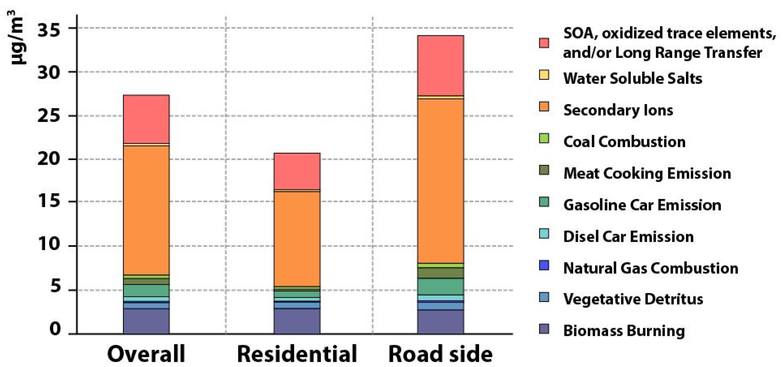
Annual average concentration of PM_2.5 in the subject area of the present study was 25.44 μg/m³, whereas those in residential area and on roads were 19.07 μg/m³ and 31.81 μg/m³, respectively. Seasonal PM_2.5 in the subject area appeared as in the following order of summer (22.71 μg/m³) > autumn (18.59 μg/m³) ≥ winter (18.50 μg/m³) > spring (16.47 μg/m³), whereas it appeared on roads as in the following order of winter (62.79 μg/m³) > spring (29.27 μg/m³) > summer (23.17 μg/m³) > autumn (12.02 μg/m³).

Annual average concentration of OC and EC in the subject area of the present study appeared as 6.37 μg/m³ and 1.50 μg/m³, respectively. The annual average concentration of OC and EC in the residential area were 4.99 μg/m³ and 1.10 μg/m³, respectively, whereas those on roads appeared as 7.75 μg/m³ and 1.91 μg/m³. In general, EC refers to the primary particles emitted from the biomass burning, coal and diesel oil, etc. [7,9]. On the contrary, OC is classified into the primary organic carbon (POC) and secondary organic carbon (SOC) according to respective processes of creation [8]. Thereby, the ratio of OC to EC as well as EC tracer method can be employed for the prediction of the ratio of SOC in OC [50]. According to the EC tracer method, the ratio of OC/EC over 2.5 is generally known that it contributes largely to the creation of the secondary OC. The ratio of annual average OC/EC appeared in residential area as 5.35, while it appeared in roads as 4.24; this suggests comparatively higher content of SOC therein.

The compounds, analyzed as an organic indicator of WIOC, were 56 compounds of PAHs and alkanes; the percentage of PAHs and alkanes to weight of PM_2.5 were 0.15% and 0.97%, respectively. PAHs are emitted through incomplete combustion of fossil fuels and biomass. In the present study, the annual average concentration of PAHs in residential area appeared as approximately 84.82 ng/m³, while it appeared on roads as 229.16 ng/m³ showing higher level of annual average concentration than that appeared in the residential area. This was estimated that it would be attributable to PAHs created from the combustion of fuels of motor vehicles that affected the area of roads. The detected seasonal concentration of PAHs commonly marked the highest level in both residential area and on roads in wintertime (residential area 43.22 ng/m³, roads 170.72 ng/m³), whereas it marked the lowest level in summertime (residential area 5.32 ng/m³, roads 5.33 ng/m³). According to previously conducted studies, the higher concentration of PAHs in wintertime was reported to be associated with the effect of phenomenon of cold ignition of vehicles; while the lower concentration of PAHs has been reported that it would be attributable to the effect of photochemical decomposition [51,52]. The varied seasonal concentration of PAHs, identified in the present study, was also estimated to be affected by effects of cold ignition of vehicles in wintertime and photochemical decomposition in summertime, as it was reported in previously conducted studies.

The sum of annual average concentration of alkanes appeared as 538 ng/m³ in residential area and 1428 ng/m³ on roads; the seasonal concentration thereof tended to show behaviors similar to seasonal variations of PAHs however the concentration in residential area appeared higher in summertime than that in wintertime. The sum of concentration of alkanes, observed in wintertime, appeared as 147 ng/m³ in residential area and 841 ng/m³ on roads; it appeared in residential area and on roads as 69 ng/m³ and 66 ng/m³, respectively, in summertime. Carbon Preference Index (CPI) signifies the ratio of concentrations of odd numbered alkanes to even numbered alkanes, wherein the C_max is defined as the number of carbons of detected peak concentration, and it represents the input of anthropogenic sources [53]. The value of CPI close to 1 in the acceptance model implies the artificial emission of fossil fuels whereas the value over 2.0 represents the alkanes originated from biomass [53,54,55].

Hopanes and steranes are the ones of organic indicators of PM_2.5 which are mainly created from fossil fuels. Therefore, the hopanes and steranes, contained in the exhaust from vehicles or thermoelectric power plants wherein fossil fuels are used, are detected comparatively in higher level [10,56,57]. A total of 16 compounds of hopanes and steranes substances including 17α(H)-22,29,30-trinorhopane, 17β(H)-21α(H)-30-norhopane and 17α(H)-21β(H)-hopane were analyzed as an ingredient of organic indicators of fossil fuels. Annual average concentration hopanes and steranes appeared in the subject area as 0.66 ng/m³ in the residential area and 2.93 ng/m³ on roads; the roads appeared with higher level of concentration.

Levoglucosan is a substance of organic indicator resulted from the biomass burning. Annual average concentration of levoglucosan in the subject area of the present study appeared as 582.75 ng/m³ (residential area) and 1007.25 ng/m³ (roads), respectively. With regard to the seasonal concentrations of levoglucosan, the highest concentration of 1173 ng/m³ appeared in residential area in autumn, while the highest concentration of 2834 ng/m³ appeared on roads in wintertime. However, the ratio of levoglucosan /OC, employed for the acceptance model, appeared higher in wintertime regardless of the area of residence or roads; the ratio of levoglucosan /OC in wintertime appeared as 272.45 mg/g (residential area) and 247.29 mg/g (on roads), respectively. Further, the ratio of K⁺/EC, the one of indicator chemical components of biomass burning, also appeared with the highest level of 0.45 (annual average 0.18) in the residential area and 0.31 (annual average 0.12) on roads in wintertime. Therefore, the biomass burning in the subject area of the present study was identified to be increasing mainly in wintertime. The cholesterol, one of WSOC, is the one of organic indicator chemical components resulted from the burning of meats [24]. Previous study had employed the ratio of cholesterol to OC for the CMB model as an indicator material of burning of meats; the ratio of cholesterol/OC used in the previously conducted study was 0.0010 [58]. The annual average concentration of cholesterol appeared as 0.20 ng/m³ in residential area and 3.86 ng/m³ on roads, respectively, in the present study. The ratio of cholesterol/OC appeared commonly below 0.0000 in all four seasons in the residential area, whereas it appeared on roads as 0.0004 in spring and 0.0010 in wintertime. In regard to the annual average concentration and seasonal concentration, the creation of PM_2.5 resulted from the burning of meats appeared higher on roads. This was attributed to the effects of restaurants placed around roads.

3.3. Source Apportionment Model

Two well-known source apportionment models (CMB and positive matrix factorization (PMF)) have been used for several decades to identify the complex sources of carbonaceous aerosols. CMB is based on an effective variance least squares (EVLS) multilinear regression method. PMF is an explicit point-by-point weighted least squares factor analysis method imposed with non-negativity constraints. Although CMB does not require a minimum set of input data, the selection of the source profile controls the model result sensitivities. The results obtained from the CMB model using the source profiles obtained in this study are presented in

Table 5. Source apportionment results of PM_2.5.

	Overall Avg		Residential Area		Roadside Area
	μg/m3	%	μg/m3	%	μg/m3	%
PM2.5 mass	27.54	100.00	20.769	100.00	34.306	100.00
Biomass burning (agricultural crop residues)	2.47	8.96	2.52	12.13	2.42	7.05
Biomass burning (forest tree types)	0.43	1.56	0.47	2.24	0..40	1.15
Vegetative detritus	0.79	2.87	0.664	3.20	0.916	2.67
Natural gas combustion	0.14	0.49	0.111	0.54	0.160	0.46
Diesel car emission	0.52	1.87	0.422	2.03	0.609	1.77
Gasoline car emission	1.32	4.79	0.726	3.49	1.914	5.58
Meat cooking emission	0.73	2.65	0.244	1.18	1.217	3.55
Coal combustion	0.40	1.44	0.325	1.57	0.469	1.37
Secondary ions	14.90	54.10	10.856	52.27	18.938	55.20
Water soluble salts	0.36	1.32	0.286	1.38	0.441	1.28
SOA, oxidized trace elements, and/or long range transfer	5.51	20.02	4.149	19.98	6.877	20.05

and Figure 5. The data, employed for the analysis conducted in the CMB model, were comprised of a total of 160 compounds including PM_2.5, OC, EC, PAHs and hopanes and steranes, etc.; the analysis of organic molecular markers of the biomass burning used the results of study presented in ‘Section 3.1’. As illustrated in the figure, the origins of PM_2.5 in the subject area of the present study appeared as in the following order: secondarily created ionic substances (54.10%) > contribution to the secondary created particulate matters and long-distance pollutants (20.02%) > biomass burning from agricultural crop residues (8.96%) and forest tree types (1.56%) (10.53%) > emission from vehicles of gasoline engine (4.79%) > Burning of meats or others in restaurants (2.65%). With regard to the comparison of residential area with the area on roads, the secondarily created ionic substances and the secondarily created particulate matters and long-distance pollutants, which occupy most origins of PM_2.5, appeared with similar rates over 72% commonly in residential area and on roads. For the case of the biomass burning, it appeared higher in the residential area (14.4%) than on roads (8.2%) due to relatively higher impacts from the open-burning of agricultural crop residues; the emission from vehicles of gasoline engine and from the burning in restaurants appeared higher on roads than those in the residential area. The rest of the burning of natural gas, combustion in coal burning thermal power plants, and water soluble ionic substances (sea-salt particulates), etc. were commonly identified as exhibiting no significant differences between residential area and on roads. In this study, there are still limitation about secondary mass from primary in the CMB result as shown in Table 5. The identified sources of secondary ions, SOA and oxidized trace elements may include mass from the primary sources such as biomass burning and car emission.

4. Conclusions

In the present study, the experimental burning of ten types of biomass were carried out to determine the organic chemical speciation using the biomass burning chamber. The results of the profile analyses were used for the identification of sources of PM_2.5 in residential area and on roads by exploiting the CMB model. The organic molecular markers for the biomass burning were identified as they were varying according to specimens of forest tree types and agricultural crop residues depending upon the hard and soft characteristics of specimens. The chemical speciation of organic molecular markers, to be varying according to respective characteristics of cultivation of burning materials, were estimated based on results of the present study. The result suggests that chemical profiles of organic molecular markers are needed according to respective crops to be cultivated and agricultural characteristics in countries to determine the organic molecular markers corresponding to biomass burning. The sources of PM_2.5 were determined based on the CMB model wherein the organic molecular markers of biomass burning, employed for the present study, were included. Major sources of PM_2.5 in the subject area of the present study appeared as sources of biomass burning, the secondary ions, secondary particulate matters, which is including long-distance transport, wherein the three sources occupied most over 84% of entire PM_2.5. In regard to the subject area distinguished into residential area and on roads, the portion of the biomass burning appeared higher in residential area than on roads. In the present study, the organic molecular markers for the biomass burning including major woods and agricultural byproducts in Korea were presented and the origins of PM_2.5 were identified via employing the CMB model exploiting data above.

References

1. The, L WHO’s global air-quality guidelines. Lancet 2006, 368, 1302. Available online: http://www.who.int/mediacentre/news/releases/2014/air-pollution/en (accessed on 21 March 2014). [CrossRef]
2. OECD, the Cost of Air Pollution. 2014. Available online: https://0-www-oecd--ilibrary-org.brum.beds.ac.uk/environment/the-cost-of-air-pollution_9789264210448-en (accessed on 21 March 2014).
3. Churg, A.; Brauer, M. Human lung parenchyma retains PM2.5. Am. J. Respir. Crit. Care Med. 1997, 155, 2109–2111. [Google Scholar] [CrossRef] [PubMed]
4. Pinkerton, K.E.; Green, F.H.; Saiki, C.; Vallyathan, V.; Plopper, C.G.; Gopal, V.; Hung, D.; Bahne, E.B.; Lin, S.S.; Ménache, M.G.; et al. Distribution of particulate matter and tissue remodeling in the human lung. Environ. Health Perspect. 2000, 108, 1063–1069. [Google Scholar] [CrossRef] [PubMed]
5. Xu, D.; Huang, N.; Wang, Q.; Liu, H. Study of ambient PM2.5 on the influence of the inflammation injury and the immune function of subchronic exposure rats. Wei Sheng Yan Jiu 2008, 37, 423–428. Available online: https://europepmc.org/article/med/18839524#impact (accessed on 1 July 2008). [PubMed]
6. Lee, Y.; Kim, E.; Oh, S.-H.; Park, M.; Chong, J.; Lee, H.; Song, H.; Kwak, N.; Lee, E.; Kim, K.; et al. Assessment between MSA and Land Originated Secondary Organic Products of PM2.5 Using LC/MSMS in Gwangju Area. J. Korean Soc. Atmos. Environ. 2019, 35, 636–646. [Google Scholar] [CrossRef]
7. Sandrini, S.; Fuzzi, S.; Piazzalunga, A.; Prati, P.; Bonasoni, P.; Cavalli, F.; Bove, M.C.; Calvello, M.; Cappelletti, D.; Colombi, C.; et al. Spatial and seasonal variability of carbonaceous aerosol across Italy. Atmos. Environ. 2014, 99, 587–598. [Google Scholar] [CrossRef]
8. Gentner, D.R.; Isaacman, G.; Worton, D.R.; Chan, A.W.H.; Dallmann, T.R.; Davis, L.; Liu, S.; Day, D.A.; Russell, L.M.; Wilson, K.R.; et al. Elucidating secondary organic aerosol from diesel and gasoline vehicles through detailed characterization of organic carbon emissions. Proc. Natl. Acad. Sci. USA 2012, 109, 18318–18323. [Google Scholar] [CrossRef] [Green Version]
9. Chow, J.C.; Watson, J.G.; Lowenthal, D.H.; Chen, L.-W.A.; Motallebi, N. Black and Organic Carbon Emission Inventories: Review and Application to California. J. Air Waste Manag. Assoc. 2010, 60, 497–507. [Google Scholar] [CrossRef]
10. Schauer, J.J.; Rogge, W.F.; Hildemann, L.M.; Mazurek, M.A.; Cass, G.R.; Simoneit, B.R.T. Source apportionment of airborne particulate matter using organic compounds as tracers. Atmos. Environ. 1996, 30, 3837–3855. [Google Scholar] [CrossRef]
11. Park, S.S.; Bae, M.-S.; Schauer, J.J.; Kim, Y.J.; Yong Cho, S.; Jai Kim, S. Molecular composition of PM2.5 organic aerosol measured at an urban site of Korea during the ACE-Asia campaign. Atmos. Environ. 2006, 40, 4182–4198. [Google Scholar] [CrossRef]
12. Schauer, J.J.; Cass, G.R. Source Apportionment of Wintertime Gas-Phase and Particle-Phase Air Pollutants Using Organic Compounds as Tracers. Environ. Sci. Technol. 2000, 34, 1821–1832. [Google Scholar] [CrossRef] [Green Version]
13. Amato, F.; Pandolfi, M.; Viana, M.; Querol, X.; Alastuey, A.; Moreno, T. Spatial and chemical patterns of PM10 in road dust deposited in urban environment. Atmos. Environ. 2009, 43, 1650–1659. [Google Scholar] [CrossRef]
14. Begum, B.A.; Biswas, S.K.; Hopke, P.K. Source Apportionment of Air Particulate Matter by Chemical Mass Balance (CMB) and Comparison with Positive Matrix Factorization (PMF) Model. Aerosol Air Qual. Res. 2007, 7, 446–468. [Google Scholar] [CrossRef] [Green Version]
15. Chow, J.C.; Watson, J.G.; Lowenthal, D.H.; Solomon, P.A.; Magliano, K.L.; Ziman, S.D.; Richards, L.W. PM10 and PM2.5 Compositions in California’s San Joaquin Valley. Aerosol Sci. Technol. 1993, 18, 105–128. [Google Scholar] [CrossRef] [Green Version]
16. Gelencsér, A.; May, B.; Simpson, D.; Sánchez-Ochoa, A.; Kasper-Giebl, A.; Puxbaum, H.; Caseiro, A.; Pio, C.; Legrand, M. Source apportionment of PM2.5 organic aerosol over Europe: Primary/secondary, natural/anthropogenic, and fossil/biogenic origin. J. Geophys. Res. Atmos. 2007, 112. [Google Scholar] [CrossRef] [Green Version]
17. Gugamsetty, B.; Wei, H.; Liu, C.-N.; Awasthi, A.; Hsu, S.-C.; Tsai, C.-J.; Roam, G.-D.; Wu, Y.-C.; Chen, C.-F. Source Characterization and Apportionment of PM10, PM2.5 and PM0.1 by Using Positive Matrix Factorization. Aerosol Air Qual. Res. 2012, 12, 476–491. [Google Scholar] [CrossRef]
18. Landis, M.S.; Patrick Pancras, J.; Graney, J.R.; White, E.M.; Edgerton, E.S.; Legge, A.; Percy, K.E. Source apportionment of ambient fine and coarse particulate matter at the Fort McKay community site, in the Athabasca Oil Sands Region, Alberta, Canada. Sci. Total Environ. 2017, 584–585, 105–117. [Google Scholar] [CrossRef]
19. Pant, P.; Harrison, R.M. Estimation of the contribution of road traffic emissions to particulate matter concentrations from field measurements: A review. Atmos. Environ. 2013, 77, 78–97. [Google Scholar] [CrossRef]
20. Vega, E.; Mugica, V.; Carmona, R.o.; Valencia, E. Hydrocarbon source apportionment in Mexico City using the chemical mass balance receptor model. Atmos. Environ. 2000, 34, 4121–4129. [Google Scholar] [CrossRef]
21. Villalobos, A.M.; Amonov, M.O.; Shafer, M.M.; Devi, J.J.; Gupta, T.; Tripathi, S.N.; Rana, K.S.; McKenzie, M.; Bergin, M.H.; Schauer, J.J. Source apportionment of carbonaceous fine particulate matter (PM2.5) in two contrasting cities across the Indo–Gangetic Plain. Atmos. Pollut. Res. 2015, 6, 398–405. [Google Scholar] [CrossRef] [Green Version]
22. Watson, J.G.; Zhu, T.; Chow, J.C.; Engelbrecht, J.; Fujita, E.M.; Wilson, W.E. Receptor modeling application framework for particle source apportionment. Chemosphere 2002, 49, 1093–1136. [Google Scholar] [CrossRef] [Green Version]
23. Yatkin, S.; Bayram, A. Source apportionment of PM10 and PM2.5 using positive matrix factorization and chemical mass balance in Izmir, Turkey. Sci. Total Environ. 2008, 390, 109–123. [Google Scholar] [CrossRef] [PubMed]
24. Skiles, M.J.; Lai, A.M.; Olson, M.R.; Schauer, J.J.; De Foy, B. Source apportionment of PM2.5 organic carbon in the San Joaquin Valley using monthly and daily observations and meteorological clustering. Environ. Pollut. 2018, 237, 366–376. [Google Scholar] [CrossRef] [PubMed]
25. Lee, S.; Russell, A.G. Estimating uncertainties and uncertainty contributors of CMB PM2.5 source apportionment results. Atmos. Environ. 2007, 41, 9616–9624. [Google Scholar] [CrossRef]
26. Park, M.; Joo, H.S.; Lee, K.; Jang, M.; Kim, S.D.; Kim, I.; Borlaza, L.J.S.; Lim, H.; Shin, H.; Chung, K.H.; et al. Differential toxicities of fine particulate matters from various sources. Sci. Rep. 2018, 8, 17007. [Google Scholar] [CrossRef]
27. Park, M.; Wang, Y.; Chong, J.; Lee, H.; Jang, J.; Song, H.; Kwak, N.; Borlaza, L.J.S.; Maeng, H.; Cosep, E.M.R.; et al. Simultaneous Measurements of Chemical Compositions of Fine Particles during Winter Haze Period in Urban Sites in China and Korea. Atmosphere 2020, 11, 292. [Google Scholar] [CrossRef] [Green Version]
28. Bae, M.-S.; Lee, T.; Schauer, J.J.; Park, G.; Son, Y.-B.; Kim, K.-H.; Cho, S.-S.; Park, S.S.; Park, K.; Shon, Z.-H. Chemical Characteristics of Size-Resolved Aerosols in Coastal Areas during KORUS-AQ Campaign; Comparison of Ion Neutralization Model. Asia-Pac. J. Atmos. Sci. 2019, 55, 387–399. [Google Scholar] [CrossRef]
29. Bae, M.-S.; Shin, J.-S.; Lee, K.-Y.; Lee, K.-H.; Kim, Y.J. Long-range transport of biomass burning emissions based on organic molecular markers and carbonaceous thermal distribution. Sci.Total Environ. 2014, 466-467, 56–66. [Google Scholar] [CrossRef]
30. Bae, M.-S.; Schwab, J.J.; Park, D.-J.; Shon, Z.-H.; Kim, K.-H. Carbonaceous aerosol in ambient air: Parallel measurements between water cyclone and carbon analyzer. Particuology 2019, 44, 153–158. [Google Scholar] [CrossRef]
31. Bae, M.-S.; Schauer, J.J.; DeMinter, J.T.; Turner, J.R.; Smith, D.; Cary, R.A. Validation of a semi-continuous instrument for elemental carbon and organic carbon using a thermal-optical method. Atmos. Environ. 2004, 38, 2885–2893. [Google Scholar] [CrossRef]
32. Watson, J.G.; Chow, J.C.; Lowenthal, D.H.; Antony Chen, L.W.; Shaw, S.; Edgerton, E.S.; Blanchard, C.L. PM2.5 source apportionment with organic markers in the Southeastern Aerosol Research and Characterization (SEARCH) study. J. Air Waste Manag. Assoc. 2015, 65, 1104–1118. [Google Scholar] [CrossRef] [Green Version]
33. Watson, J.G.; Chow, J.C.; Lu, Z.; Fujita, E.M.; Lowenthal, D.H.; Lawson, D.R.; Ashbaugh, L.L. Chemical Mass Balance Source Apportionment of PM10 during the Southern California Air Quality Study. Aerosol Sci. Technol. 1994, 21, 1–36. [Google Scholar] [CrossRef] [Green Version]
34. Han, Y.M.; Chen, L.W.A.; Huang, R.J.; Chow, J.C.; Watson, J.G.; Ni, H.Y.; Liu, S.X.; Fung, K.K.; Shen, Z.X.; Wei, C.; et al. Carbonaceous aerosols in megacity Xi’an, China: Implications of thermal/optical protocols comparison. Atmos. Environ. 2016, 132, 58–68. [Google Scholar] [CrossRef]
35. Chen, Y.; Tian, C.; Feng, Y.; Zhi, G.; Li, J.; Zhang, G. Measurements of emission factors of PM2.5, OC, EC, and BC for household stoves of coal combustion in China. Atmos. Environ. 2015, 109, 190–196. [Google Scholar] [CrossRef]
36. Guofeng, S.; Siye, W.; Wen, W.; Yanyan, Z.; Yujia, M.; Bin, W.; Rong, W.; Wei, L.; Huizhong, S.; Ye, H.; et al. Emission Factors, Size Distributions, and Emission Inventories of Carbonaceous Particulate Matter from Residential Wood Combustion in Rural China. Environ. Sci. Technol. 2012, 46, 4207–4214. [Google Scholar] [CrossRef] [Green Version]
37. He, L.-Y.; Hu, M.; Zhang, Y.-H.; Huang, X.-F.; Yao, T.-T. Fine Particle Emissions from On-Road Vehicles in the Zhujiang Tunnel, China. Environ. Sci. Technol. 2008, 42, 4461–4466. [Google Scholar] [CrossRef]
38. Sun, J.; Shen, Z.; Cao, J.; Zhang, L.; Wu, T.; Zhang, Q.; Yin, X.; Lei, Y.; Huang, Y.; Huang, R.J.; et al. Particulate matters emitted from maize straw burning for winter heating in rural areas in Guanzhong Plain, China: Current emission and future reduction. Atmos. Res. 2017, 184, 66–76. [Google Scholar] [CrossRef]
39. Mason, P.E.; Darvell, L.I.; Jones, J.M.; Williams, A. Observations on the release of gas-phase potassium during the combustion of single particles of biomass. Fuel 2016, 182, 110–117. [Google Scholar] [CrossRef] [Green Version]
40. Sorvajarvi, T.; DeMartini, N.; Rossi, J.; Toivonen, J. In situ measurement technique for simultaneous detection of K, KCl, and KOH vapors released during combustion of solid biomass fuel in a single particle reactor. Appl. Spectrosc 2014, 68, 179–184. [Google Scholar] [CrossRef]
41. Ni, H.; Tian, J.; Wang, X.; Wang, Q.; Han, Y.; Cao, J.; Long, X.; Chen, L.W.A.; Chow, J.C.; Watson, J.G.; et al. PM2.5 emissions and source profiles from open burning of crop residues. Atmos. Environ. 2017, 169, 229–237. [Google Scholar] [CrossRef]
42. Dotaniya, M.L.; Meena, V.D.; Basak, B.B.; Meena, R.S. Potassium Uptake by Crops as Well as Microorganisms. In Potassium Solubilizing Microorganisms for Sustainable Agriculture; Meena, V.S., Maurya, B.R., Verma, J.P., Meena, R.S., Eds.; Springer India: New Delhi, India, 2016; pp. 267–280. [Google Scholar] [CrossRef]
43. Kang, S.R.; Cho, W.; Na, M.-H.; Choi, D.W. Consideration of Environmental Factors and Growth Factors and Watering Facilities for Prediction of Pepper Production. J. Korean Data Anal. Soc. 2020, 22, 177–188. Available online: http://scholar.dkyobobook.co.kr/searchDetail.laf?barcode=4010027613851 (accessed on 28 February 2020). [CrossRef]
44. Achad, M.; Caumo, S.; De Castro Vasconcellos, P.; Bajano, H.; Gómez, D.; Smichowski, P. Chemical markers of biomass burning: Determination of levoglucosan, and potassium in size-classified atmospheric aerosols collected in Buenos Aires, Argentina by different analytical techniques. Microchem. J. 2018, 139, 181–187. [Google Scholar] [CrossRef]
45. Simoneit, B.R.T.; Schauer, J.J.; Nolte, C.G.; Oros, D.R.; Elias, V.O.; Fraser, M.P.; Rogge, W.F.; Cass, G.R. Levoglucosan, a tracer for cellulose in biomass burning and atmospheric particles. Atmos. Environ. 1999, 33, 173–182. [Google Scholar] [CrossRef]
46. Mkoma, S.L.; Kawamura, K.; Fu, P.Q. Contributions of biomass/biofuel burning to organic aerosols and particulate matter in Tanzania, East Africa, based on analyses of ionic species, organic and elemental carbon, levoglucosan and mannosan. Atmos. Chem. Phys. 2013, 13, 10325–10338. [Google Scholar] [CrossRef] [Green Version]
47. Fu, P.; Kawamura, K.; Chen, J.; Miyazaki, Y. Secondary Production of Organic Aerosols from Biogenic VOCs over Mt. Fuji, Japan. Environ. Sci. Technol. 2014, 48, 8491–8497. [Google Scholar] [CrossRef]
48. Ho, K.F.; Engling, G.; Sai Hang Ho, S.; Huang, R.; Lai, S.; Cao, J.; Lee, S.C. Seasonal variations of anhydrosugars in PM2.5 in the Pearl River Delta Region, China. Tellus B: Chem. Phys. Meteorol. 2014, 66, 22577. [Google Scholar] [CrossRef]
49. Fine, P.M.; Cass, G.R.; Simoneit, B.R.T. Organic compounds in biomass smoke from residential wood combustion: Emissions characterization at a continental scale. J. Geophys. Res. Atmos. 2002, 107, ICC 11-1–ICC 11-9. [Google Scholar] [CrossRef]
50. Turpin, B.J.; Huntzicker, J.J. Identification of secondary organic aerosol episodes and quantitation of primary and secondary organic aerosol concentrations during SCAQS. Atmos. Environ. 1995, 29, 3527–3544. [Google Scholar] [CrossRef]
51. Arhami, M.; Minguillón, M.C.; Polidori, A.; Schauer, J.J.; Delfino, R.J.; Sioutas, C. Organic compound characterization and source apportionment of indoor and outdoor quasi-ultrafine particulate matter in retirement homes of the Los Angeles Basin. Indoor Air 2010, 20, 17–30. [Google Scholar] [CrossRef] [Green Version]
52. Lee, S.C.; Ho, K.F.; Chan, L.Y.; Zielinska, B.; Chow, J.C. Polycyclic aromatic hydrocarbons (PAHs) and carbonyl compounds in urban atmosphere of Hong Kong. Atmos. Environ. 2001, 35, 5949–5960. [Google Scholar] [CrossRef]
53. Simoneit, B.R.T. Organic matter of the troposphere—V: Application of molecular marker analysis to biogenic emissions into the troposphere for source reconciliations. J. Atmos. Chem. 1989, 8, 251–275. [Google Scholar] [CrossRef]
54. Rogge, W.F.; Hildemann, L.M.; Mazurek, M.A.; Cass, G.R.; Simoneit, B.R.T. Sources of fine organic aerosol. 2. Noncatalyst and catalyst-equipped automobiles and heavy-duty diesel trucks. Environ. Sci. Technol. 1993, 27, 636–651. [Google Scholar] [CrossRef]
55. Xiong, Y.; Zhou, J.; Schauer, J.J.; Yu, W.; Hu, Y. Seasonal and spatial differences in source contributions to PM2.5 in Wuhan, China. Sci. Total Environ. 2017, 577, 155–165. [Google Scholar] [CrossRef] [PubMed]
56. Rogge, W.F.; Hildemann, L.M.; Mazurek, M.A.; Cass, G.R.; Simoneit, B.R.T. Sources of Fine Organic Aerosol. 8. Boilers Burning No. 2 Distillate Fuel Oil. Environ. Sci. Technol. 1997, 31, 2731–2737. [Google Scholar] [CrossRef]
57. Simoneit, B.R.T. A review of biomarker compounds as source indicators and tracers for air pollution. Environ. Sci. Pollut. Res. 1999, 6, 159–169. [Google Scholar] [CrossRef]
58. Rogge, W.F.; Hildemann, L.M.; Mazurek, M.A.; Cass, G.R.; Simoneit, B.R.T. Sources of fine organic aerosol. 1. Charbroilers and meat cooking operations. Environ. Sci. Technol. 1991, 25, 1112–1125. [Google Scholar] [CrossRef]
Figure 1. Schematic diagram of biomass burning chamber.
Applsci 10 04449 g001
Figure 2. Relative chemical abundances in PM2.5 and scatterplots between measured and reconstructed PM2.5 mass from burning of forest tree types and agricultural crop residues byproducts.
Applsci 10 04449 g002
Figure 3. Composition ratio of PM2.5 mass by biomass burning of woods and agricultural byproducts.
Applsci 10 04449 g003aApplsci 10 04449 g003b
Figure 4. Comparison of concentrations of the main components of PM2.5 from forest burning and agriculture burning.
Applsci 10 04449 g004
Figure 5. Source apportionment results of PM2.5.
Applsci 10 04449 g005