Improvement of Learning Stability of Generative Adversarial Network Using Variational Learning

Department of Computer Science and Engineering, Dankook University, Yongin-si, Gyeonggi-do 16890, Korea
*
Author to whom correspondence should be addressed.
Appl. Sci. 2020, 10(13), 4528; https://0-doi-org.brum.beds.ac.uk/10.3390/app10134528
Submission received: 14 May 2020
/
Revised: 23 June 2020
/
Accepted: 26 June 2020
/
Published: 30 June 2020
(This article belongs to the Special Issue Deep Learning Applied to Image Processing)
Abstract
:In this paper, we propose a new network model using variational learning to improve the learning stability of generative adversarial networks (GAN). The proposed method can be easily applied to improve the learning stability of GAN-based models that were developed for various purposes, given that the variational autoencoder (VAE) is used as a secondary network while the basic GAN structure is maintained. When the gradient of the generator vanishes in the learning process of GAN, the proposed method receives gradient information from the decoder of the VAE that maintains gradient stably, so that the learning processes of the generator and discriminator are not halted. The experimental results of the MNIST and the CelebA datasets verify that the proposed method improves the learning stability of the networks by overcoming the vanishing gradient problem of the generator, and maintains the excellent data quality of the conventional GAN-based generative models.
1. Introduction
The generative adversarial network (GAN) [1] is a deep generative model that is composed of artificial neural networks. Numerous studies have recently been undertaken on GAN in various fields based on the use of generative models, such as super resolution [2], image translation [3], medical image analysis [4], and three-dimensional (3D) modelling [5]. GAN has a structure that comprises two competing models—referred to as the discriminator and generator—that learn from each other. When it was first introduced, it gained considerable attention by researchers because it produced results with considerably higher quality (more realistic, higher resolution) as compared to many conventional generative models. However, given that the learning of networks could become unstable, owing to the competitive learning structure used in GAN, it was necessary to either a) apply techniques, such as the deep convolutional generative adversarial network (DCGAN) [6], or b) undergo a tedious hyperparameter tuning process [7] to achieve the learning of GAN. The widespread use of GAN is restricted by these issues, and research on various methods to resolve them is ongoing.
The most common cause of the unstable learning of GAN is the so-called ‘vanishing gradient’ [8], whereby th gradient vanishes during the learning process of the generator for generating new samples that can deceive the discriminator. This occurs when the discriminator reaches the local optimum [9]. The learning of early GAN models was performed based on the minimization of the Jensen Shannon divergence (JSD) between the distribution of real data and the distribution the generator. Herein, the JSD does not converge when the intersection set of the support of the two compared distributions is the null set. This leads to a learning failure for GAN. Research studies that were conducted on the least-squares generative adversarial network (LSGAN) [10], Wasserstein generative adversarial network (WGAN) [11], Wasserstein generative adversarial network-gradient penalty (WGAN-GP) [9], f-GAN [12], and on the deep regret analytic generative adversarial network (DRAGAN) [13], attempted to improve the performance of GAN by solving the vanishing gradient problem by replacing the JSD following the identification of a new divergence that could always converge. However, experiments on extensive hyperparametric searches while using the same dataset and architecture [7] showed that the algorithmic differences of these GAN did not significantly improve the original GAN. A study on an energy-based generative adversarial network (EBGAN) [14] proposed a method that stabilized energy based on reconstruction errors by designing the discriminator as an autoencoder structure. A boundary equilibrium generative adversarial network (BEGAN) [15] was inspired by WGAN and EBGAN, and it produced high-quality data. A representative feature-based generative adversarial network (RFGAN) [16] improved the learning stability of GAN based on the use of a pretrained autoencoder to provide the discriminator with representative features for training data. Salimans et al. [17] analyzed the vanishing gradient of GAN more systematically and suggested a few methods to solve the ‘vanishing gradient’ problem, yet the approach was not able to solve the problem that occurred in real problems.
Some other studies proposed a model that combined the variational autoencoder (VAE) [18], another generative model with GAN, which resulted in the improvement of the learning stability of networks. VAE shows low performance (e.g., blurry results for image data) in many cases in terms of the quality of the generated data compared to GAN, yet ensures a stable convergence and yields a better likelihood than GAN [19]. By applying these characteristics of VAE to GAN, the adversarial autoencoder (AAE) [20] and adversarial variational Bayes (AVB) [21] models were combined based on the use of the GAN discriminator instead of the Kullback–Leibler divergence (KLD) that was used as regularizer in the objective function of VAE. In [22], a GAN model was introduced that combined the reconstruction, GAN, and classification losses of the pretrained classifier. VAE–GAN [23] improved the image quality of VAE based on the use of the discriminator to separate the perceptual information [24] of the input and output instead of using the reconstruction loss between the input and output data in the structure of VAE. Adversarially learned inference (ALI) [25] and bidirectional GAN (BIGAN) [26] combined the autoencoder and GAN based on the use of an adversarial learning method, whereby the encoder and decoder generated fake data and fake code, respectively, and the discriminator identified whether data and code were one pair or not. Adversarial symmetric AS–VAE [27] learned the symmetric VAE with the adversarial learning method of ALI. Hu et al. [28] found the mathematical linkages and similarities between VAE and GAN, and showed that VAE can be expressed as the GAN formula, which included the perfect discriminator (i.e., fully learned the ideal discriminator). Furthermore, at the same time, they proved that various methods, such as the importance weighting method that is used to improve VAE, could be applied to GAN. Rosca et al. [29] revealed the possibility of combining variational inference with GAN, and proposed the -GAN method that solves the mode collapse of the generator by combining AAE and GAN. DeePSiM [30] proposed a loss function that can generate clear data by combining the pixel-wise reconstruction loss of VAE, the perceptual loss obtained from feature space, and the adversarial loss obtained by inserting the generated and real data into the discriminator. CycleGAN [31] has a structure that translates data into each domain for paired datasets that are based on the use of two GANs and reconstruction errors. In this study, its structure is similar to that of -GAN based on the assumption that one of the domains is a latent space domain.
In this paper, we propose a generative adversarial model using variational learning to improve the learning stability of GAN. We conceived this idea based on the common properties of the GAN generator and the VAE decoder that aided the identification of an approximate distribution of the original data distribution. Based on the assumption that the prior distribution of VAE is equal to the noise distribution of GAN, we built a combined model that was composed of the encoder, generator, and discriminator. The proposed method obtained the latent code based on the use of a reparameterization trick after inputting the given data into the VAE encoder along with the learning of GAN, and generated new data by inputting this latent code in the GAN generator. Subsequently, it trained the GAN generator along with the VAE encoder based on the use of the input data, and generated data and latent code with the loss of VAE.
Unlike the conventional methods that extracted better features or found a mathematical linkage between two models that were based on the combination of GAN and VAE, the proposed method focused on the solution of the vanishing gradient problem of GAN and used VAE as an auxiliary model for GAN. Given that this structure does not change the model structure or the input/output forms of the conventional GAN, it has the advantage that it can be naturally applied to problems that to-this-date have utilized GAN. In addition, by solving the vanishing gradient problem of GAN according to economic terms, we built simpler and more efficient networks based on the use of the VAE structure instead of the AAE structure [29].
Finally, we conducted experiments in order to observe the occurrence of the vanishing gradient for the MNIST dataset [32] that contained handwritten images, and the CelebA dataset [33] that was made up of facial images of celebrities, which were extensively used in the GAN evaluation. Based on quantitative evaluations, such as sample generation and latent space walk, and based on a qualitative evaluation, such as the multiscale structural SIMilarity (MS-SSIM), we were able to verify that the proposed method improved the learning stability by preventing the vanishing gradient, while, at the same time, maintained the performance of the conventional GAN in terms of the quality of the resulting images.
This paper is structured, as follows. Section 2 introduces GAN and VAE that are important latent variable models that constitute the basis for the proposed method. Section 3 proposes a new combined structure and its loss function, and a learning algorithm to solve the vanishing gradient of GAN based on the use of VAE. Section 4 verifies the effectiveness of the proposed method through experiments and compares it with the conventional models. Section 5 presents the conclusions that are drawn from this study.
2. Preliminary Works
2.1. Generative Adversarial Networks
GAN consists of two types of artificial neural network models, that is, the discriminator and the generator. The generator learns to be able to create fake data to the degree that the discriminator can regard the generated data as real data, and the discriminator learns to be able to discriminate between real data and fake data that are generated by the generator. In this way, the generator and the discriminator achieve their objective by competing with each other based on opposing goals. This competition structure can be expressed as a minimax game, as follows:
Herein, G is the generator and D is the discriminator. The generator is a neural network model that generates fake data with a latent variable z as the input sampled from distribution , which was assumed as the prior. Additionally, is a parameter of the generator network. The discriminator is a neural network model which serves as a classifier that discriminates between real data and fake data generated from the generator, and it can be expressed as . In this instance, is a parameter of the discriminator’s network. Additionally, y is the output of the discriminator and outputs zero if the discriminator regards the sample as fake data, or outputs unity values if the discriminator regards the sample as real data. The minimax game of Equation (1) is a loss for the discriminator and a loss for the generator and can be decomposed, as follows.
By using Equation (2), the discriminator can update to minimize the binary cross entropy for data and . By using Equation (3), the generator can update to increase the probability that the discriminator regards fake data as real data, that is, to generate fake data that are very similar to the actual data.
As the learning progresses, if becomes equal to and reaches the optimum, then the discriminator can no longer discriminate between real data and fake data that are generated by the generator. At this point, the minimax game of Equation (1) reaches the Nash equilibrium and learning is complete. If the discriminator is always optimum for the generator during the learning, that is, if the discriminator can always perfectly discriminate between real and fake data, then the result of the minimax game is equivalent to the minimization of the Jensen Shannon divergence (JSD) [34] of and . Correspondingly, there is always a unique solution to this [1]. However, in the actual learning of GAN, it is practically difficult to find the optimum discriminator for the generator at every learning step. Therefore, learning should be done by alternating the generator and the discriminator.
2.2. Variational Autoencoder
The variational autoencoder (VAE) is a deep generative model that consists of two neural networks, that is, an encoder and a decoder. The objective of VAE is to find a parameter that maximizes the likelihood of the approximate distribution , which approximates the original data distribution . To solve this problem, it is assumed that is a latent variable model with a latent variable z. Accordingly, it can be expressed as a joint distribution, as follows:
To allow for the application of the logarithm on both sides of Equation (4), an arbitrary distribution is introduced for z to make the calculation easier. Using , Equation (4) can be decomposed as follows.
The second term on the right side of Equation (5) can be expressed according to Equation (7) while using the KLD, whereby [35] indicates how similar and are.
The KLD is always ≥ 0, and it has a characteristic of being zero when . Therefore, the first term on the right side of Equation (5) can be considered as the lower bound of and can be expressed, as follows:
Using Equations (6) and (7), Equation (5) can be rewritten as follows.
If is tractable, can be replaced by , the KLD becomes zero, then is equal to . In this case, the solution of Equation (8) can be obtained while using the expectation-maximization (EM) algorithm [36].
However, if is intractable, then the solution cannot be obtained. In this case, is assumed to be the distribution that approximates . This is called variational inference.
It approximates , which is necessary for the calculation of based on the use of the artificial neural network with parameter as , and with periodic updating of . Given that is intractable in variational inference, it is not possible to update while directly minimizing , yet the solution can be obtained by updating to maximize the lower bound . Therefore, the loss function of VAE is as follows.
The second term on the right side of Equation (9) is a metric that shows how well the input x is restored owing to the reconstruction loss in the autoencoder. The first term shows how similar the distribution of the inference model and the given prior are. Minimizing these two terms at the same time is equivalent to minimizing . The VAE learnt in this way generates new data by inputting into the decoder. Experimentally, the method of multiplication of the regularization term with the use of the appropriate weight in VAE [37] is known to be helpful for the learning of VAE. Thus, the loss function of VAE can be finally written, as follows.
3. Improving the Learning Stability of Generative Adversarial Networks Using Variational Learning
3.1. Problem Statement
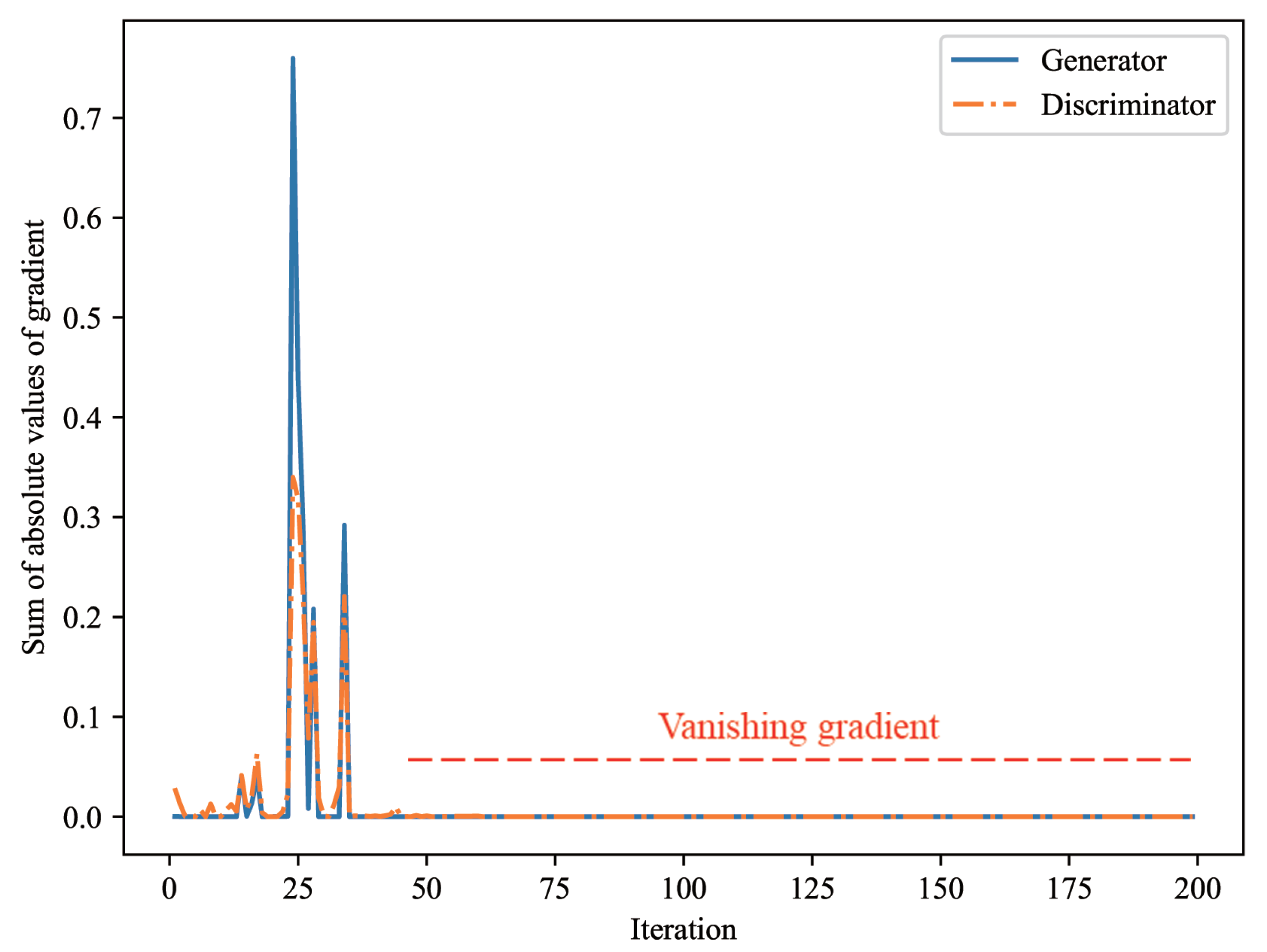
As indicated previously, it was proved that there was a unique solution of the minimax game of Equation (1) if the optimal discriminator could always be obtained for the generator during the learning of GAN [1]. However, in the learning process of GAN, if the discriminator approaches the local optimum, the gradient of the generator can vanish without reaching a unique solution. The generator deals with the challenging problem of generating high-dimensional data of excellent quality that is difficult to be distinguished from real data. Conversely, given that the discriminator deals with the relatively easy problems of discriminating between real and low-quality data generated by the generator early in the learning process, the learning of the discriminator often converges much faster than that of the generator. In this case, the discriminator can be close to the local optimum. This results in a vanishing gradient that occurs in the generator. As the weights of the generator are updated by the backpropagation algorithm during the learning of GAN, the generator generates fake data that are closer to real data. Given that the generated fake data reduce the accuracy of the learning of the discriminator up to that point, the learning of the discriminator continues. The discriminator again provides a new learning standard for the generator, and the learning of GAN thus continues. However, when the gradient of the generator vanishes owing to the reason described above, the quality of the fake data generated by the generator no longer improve. Consequently, the learning of the discriminator also halts and, in the end, the learning of GAN fails. Figure 1 shows an example of the vanishing gradient of the generator during the learning process of GAN for the CelebA dataset [33].
We trained GAN using a pretrained discriminator to artificially create a situation where the discriminator performed better than the generator, and observed that the gradient vanished from the generator, as shown in Figure 1.
To solve the vanishing gradient problem, Goodfellow et al. [1] used Equation (11) in the learning of the generator by slightly modifying the original objective function of Equation (3).
However, Arjovsky et al. [38] indicated that the modification of the objective function contributed to the generation of good-quality data and facilitated early learning, yet caused mode collapse and destabilized learning. Moreover, the vanishing gradient problem was still observed when these alternative objective functions were applied to real problems [11].
3.2. Hybrid Generative Adversarial Networks for Solving Vanishing Gradient Problem
GAN and VAE are generative models that generate new data samples that are based on learning networks. Each model is applied to different problems according to the difference in its characteristics, and has been developed by reinforcing its advantages and by compensating for its disadvantages. Both GAN and VAE are latent variable models, and they both use secondary networks to optimize the models. Conversely, there are differences between the two models in the way learning is conducted, the quality of the results, and the learning stability. Based on these common characteristics and differences between the two models, and by enabling the two models to complement each other, we designed the network, so that it can produce high-quality data and achieve stable learning.
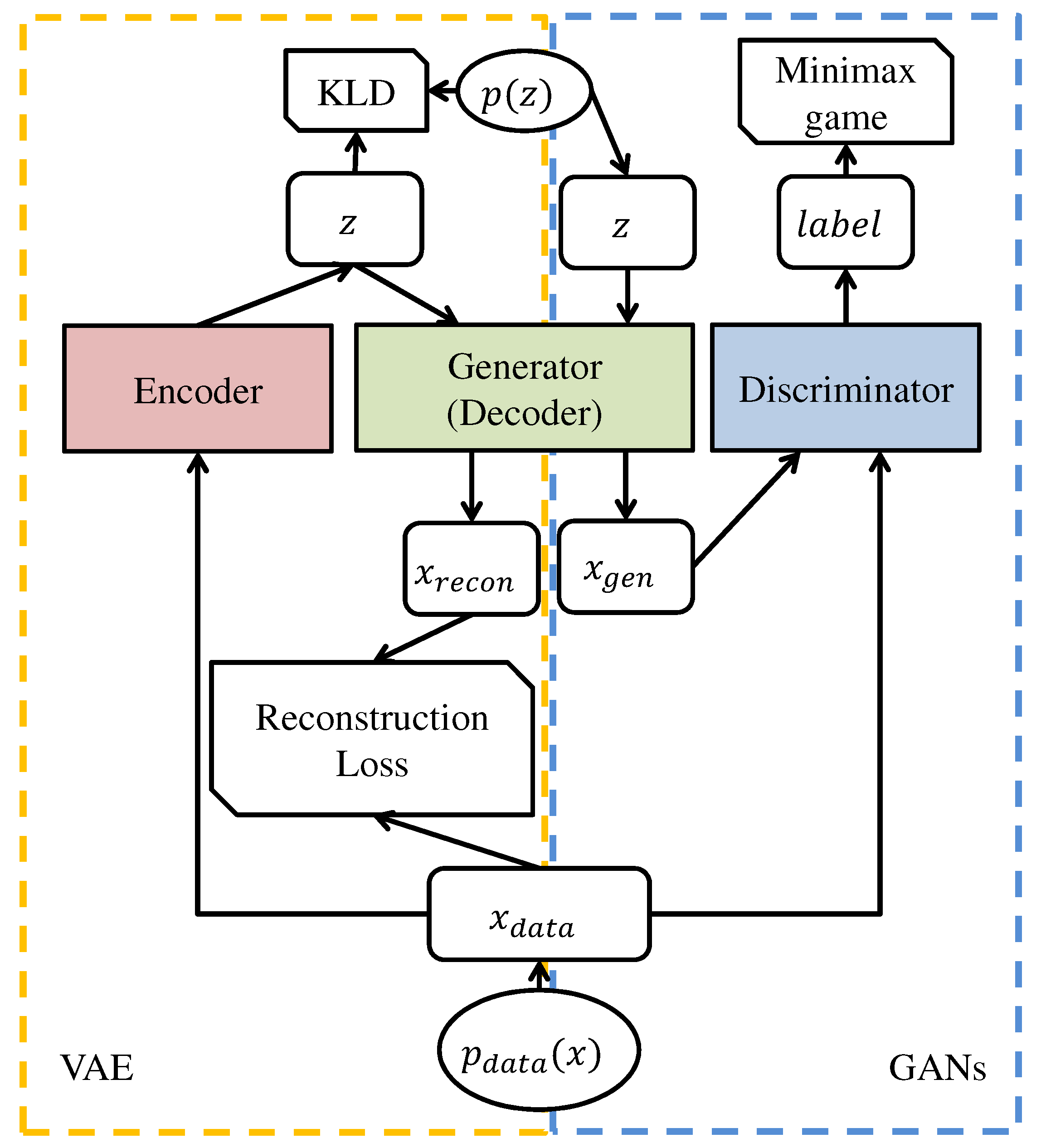
Assuming that GAN and VAE have the same prior, the GAN generator and the VAE decoder have the same structure and objective. Despite the differences in the forms of the VAE objective function of Equation (10) and the GAN objective function of Equation (1), both approximated the distribution of real data () with the use of artificial neural networks. Both of the models generated new data x from the already known (and easy to sample) latent variable zm, just like standard isotropic Gaussian data after learning. Figure 2 shows the structure of GAN and VAE and the process of generating new data using each model. Figure 2a,c, respectively, visualize the structures of GAN and VAE with the use of a diagram. In the figures, the discriminator, generator, encoder, and decoder blocks denote the corresponding deep neural network. The terms and , respectively, denote the real data and the fake data generated by the generator, and z is a latent variable.
Additionally, , , and are probability distribution functions for the real data, generated data, and latent variable, respectively. Figure 2 illustrates that both of the models have a structure where the secondary network is added to the neural network which corresponds to the generative model. Figure 2b,d visualize an inference model that generates data using the trained GAN and VAE based on a diagram. Figure 2a,c illustrate that the process of generating data using the trained model is the same for GAN and VAE.
The trained VAE decoder plays the same role as the GAN generator. The objective function of the VAE decoder converges much faster than that of the GAN generator, and generates data with the characteristics of the original data from the initial learning stage. Furthermore, unlike GAN, in which the generator and the discriminator interfere with each other’s objectives and learn competitively, the VAE encoder and decoder learn cooperatively to satisfy the same objective function. Therefore, unlike the GAN generator that varies considerably, depending on the state of the discriminator—that is the secondary network of the generator—the VAE decoder continually maintains a stable gradient, regardless of the current state of the encoder—that represents the secondary network of the decoder. Based on these characteristics of GAN and VAE, we propose GAN while using variational learning (VLGAN). By performing the learning of GAN and VAE simultaneously, the proposed method helped the discriminator escape from the local optimum based on the use of the gradient maintained in the VAE decoder, despite the fact that the vanishing gradient problem occurred in the learning of the generator, owing to the occurrence of the local optimum in the GAN discriminator.
Figure 3 shows the structure of the proposed VLGAN. VLGAN is composed of three artificial neural networks, that is, the generator, discriminator, and encoder, parameterized by ,,. To learn the proposed structure, we propose an algorithm that accomplishes the dual learning of the model, which corresponds to the generator (decoder), based on the use of both the loss function of GAN (Equation (1)) and the loss function of VAE (Equation (10)).
First, it builds a mini-batch with M new data for VAE and GAN for each iteration. In the learning of VAE, M data are input through the encoder , which yield z with the noise distribution based on the standard isotropic Gaussian and the reparameterization trick [18] (the dimension of z is L). Subsequently, the restored data x pass through the decoder , which approximates the expected value of Equation (9) by the Monte-Carlo estimation method [39].
Parameters and are updated by the SGD algorithm or the Adagrad algorithm or the ADAM algorithm using Equation (12) as the loss function. In the learning of GAN, M fake data are generated by the generator from M data and M noise data sampled using a given prior . After this, the expected value of Equation (2) is approximated based on a Monte–Carlo estimation process using the real data, , and the generated fake data.
The discriminator is learnt by updating to minimize Equation (13) (in this experiment, the hyperparameter k was set to 1). Lastly, for the learning of the generator of GAN, M fake data are generated by the generator from the M noise data sampled while using the given prior . Accordingly, by using the discriminator learned in the previous step, the expected value of Equation (3) is approximated based on a Monte–Carlo estimation.
The parameter is updated to minimize Equation (14). The algorithm of the proposed method (VLGAN) is summarized in Algorithm 1.
| Algorithm 1 The number of steps to apply to the discriminator, k, is a hyperparameter. We used , the least expensive option, in our experiments. is a hyperparameter. M is the batch size. ,, are parameters for generator, encoder, and discriminator, respectively. is 0 or 1. |
|
4. Experimental Results and Discussions
4.1. Dataset and Model Configuration
To evaluate the performance of the proposed method, we conducted experiments with the MNIST [32] and the CelebA datasets [33] that are mainly used to compare the performances of models in the field of computer vision. The MNIST dataset consists of 60,000 handwritten images using the Arabic numerals from 0 to 9. The CelebA dataset contains facial images of celebrities and consists of a total of 202,599 images. All the data samples of the studied datasets were normalized to have zero means and unit standard deviations based on the mean and standard deviation of the training set. Facial images of the CelebA dataset were resized to 64 × 64 after the facial area was aligned based on the eye coordinates, which were identified manually. All of the data samples included in each dataset were subdivided based on the ratio of 4:1:1, and the data segments were used as the training, validation, and test sets, respectively.
We designed the network for the experiments based on the structure of DCGAN [6] that is used in many studies on the MNIST and CelebA datasets. The latent variable was set to have dimensions of two and 64 in the cases of the MNIST and the CelebA datasets, respectively. The weights of each model were initialized using the Xavier method [40]. The adaptive momentum optimizer (ADAM) [41] was used to optimize the weight of the network in our experiments (other methods for weight initialization and optimization can be also applied to the proposed method). The hyperparameter of ADAM, , was set to (0.5, 0.999). We used 0.0002 as the learning rate of the generator and encoder, and 0.002 as the learning rate of the discriminator.
4.2. Improving Learning Stability Using the Proposed Method
The main reason for the vanishing gradient in the learning process of GAN is that the discriminator is learnt so fast that the performance between the generator and the discriminator are not balanced. Therefore, we first established a strong discriminator that was able to discriminate the fake data generated by the generator based on the learning of the discriminator with 10 epochs to verify whether the proposed method can solve the problem of the vanishing gradient. Subsequently, DCGAN and the proposed VLGAN were learnt again afresh with the use this strong discriminator as the initial value. Figure 4 shows the experimental results for the MNIST and the CelebA datasets. It is confirmed that the gradient of the generator approaches zero (i.e., vanishes) within around 50 iterations, as shown in Figure 4a,c. Conversely, in the case of learning, which was based on the use of VLGAN (Figure 4b,d), the generator could continue to use the gradient received from the VAE decoder, even when the gradient vanished in the loss of GAN owing to the strength of the discriminator. Consequently, the learning of GAN continued and was unaffected by the vanishing gradient problem.
4.3. Quality of Data Generated by the Proposed Method
We evaluated the quality of the data generated based on the use of the proposed method and compared the performance of the proposed method with that of the DCGAN [6], and -GAN [29], which attempted to improve the learning stability of GAN. Figure 5 shows newly generated image data after learning with the use of images from the CelebA dataset and the MNIST dataset with each of the referred methods. In Figure 5, it is shown that both the proposed and conventional methods, which were based on GAN, generated good quality data, as confirmed by the naked eye.
We evaluated the quality of each method using the latent space walk (LSP) method [1]. The LSP can be used to verify whether the deep generative model is overfitting the actual data. This can be achieved by observing the aspect of the data generated by the latent variables, as the latent variable a gradually changes toward the other latent variable b in the latent space. To address this issue, the model first underwent learning with the use of the training data, and then recorded the latent variables that produced two samples based on the sampling of two data units from the trained model denoted as a and b. In the latent space, we observed the data that were generated by the generator using variable values along a straight line between points a and b. Accordingly, if there was a semantically natural change between the data generated by the generator with values that corresponded to a and b, then the generator was not overfitting. Figure 6a,b show the LSP results using the proposed VLGAN for the CelebA dataset and the MNIST dataset, respectively. Relative to the images at the top left (A), top right (B), bottom left (C), and the bottom right (D) in Figure 6, the generated images show that the semantic aspect of changes is well presented among the reference images as the latent variables change.
We measured the multi-scale structural similarity (MS–SSIM) [42] for the generated images and the training time taken by each method for single iteration to quantitatively evaluate the performance of each method (Figure 7). The MS-SSIM is extensively used for evaluating image quality, and takes values between 0 and 1. Given that the MS–SSIM measures the similarity between images belonging to the same category, we conducted experiments only for the CelebA dataset that has the same property for face. The MS–SSIM indicates that the similarity between the two images is higher as the resulting value becomes closer to one. Figure 7 shows that the proposed method is slightly slower than DCGAN in terms of speed, yet the MS–SSIM value was slightly higher than that of DCGAN in terms of image quality. Conversely, in comparison with -GAN, -GAN yields slightly higher MS–SSIM values compared to VLGAN, yet VLGAN is two times faster than -GAN in terms of speed. This is because -GAN learns the generator again by using the restored data as the input of GAN using AAE. Therefore, additional discriminator models and additional learning about them are required in the execution process of AAE. The results of Figure 7 confirm that, when the simplicity of the model and the trade-off between the training speed and image quality are considered, the proposed method efficiently maintains the data quality achieved by GAN, while it simultaneously improves the learning stability with a low-calculation cost.
5. Conclusions
The so-called ’vanishing gradient’ is one of the typical problems of GAN. In this paper, we proposed a VLGAN that improved the learning stability, while it maintained the quality of the data that were generated using variational learning. In the proposed method, VAE was utilized to stably provide supplementary gradient to GAN. Therefore, even when the gradient of the generator vanished owing to the learning imbalance between the discriminator and the generator, learning was maintained in a stable form by receiving the gradient from the VAE decoder. The proposed method used the VAE encoder model as the secondary model, while it maintained the basic structure of the conventional GAN. Therefore, it can be easily applied to improve the learning stability of various types of GAN-based models that have already been developed. The experimental results of the MNIST and the CelebA datasets that were extensively used in prior research studies on computer vision technology with deep learning verified that the proposed method overcame the vanishing gradient problem and, at the same time, achieved excellent data generation performance of GAN. The proposed method is expected to help solve the mode collapse problem that often occurs in the learning process of GAN, given that the loss of VAE forces learning for all diverse situations. In the future, we will conduct experiments and additional research on the mode collapse problem.
Author Contributions
J.-Y.L. and S.-I.C. participated in the study design, contributed to the formal analysis, data collection, validation, drafted the manuscript and edited the draft. All authors approved the final version of the manuscript.
Funding
This work was supported in part by the National Research Foundation of Korea Grant through the Korean Government (MSIT) under Grant 2018R1A2B6001400, and in part by the Human Resources Program in Energy Technology of the Korea Institute of Energy Technology Evaluation and Planning from the Ministry of Trade, Industry and Energy, South Korea, under Grant 20174030201740.
Conflicts of Interest
The authors declare no conflict of interest.
References
- Goodfellow, I.; Pouget-Abadie, J.; Mirza, M.; Xu, B.; Warde-Farley, D.; Ozair, S.; Courville, A.; Bengio, Y. Generative adversarial nets. In Proceedings of the Neural Information Processing Systems, Montreal, QC, Canada, 8–13 December 2014; pp. 2672–2680. [Google Scholar]
- Ledig, C.; Theis, L.; Huszár, F.; Caballero, J.; Cunningham, A.; Acosta, A.; Aitken, A.; Tejani, A.; Totz, J.; Wang, Z.; et al. Photo-realistic single image super-resolution using a generative adversarial network. In Proceedings of the IEEE Conference on Computer Vision and Pattern Recognition, Honolulu, HI, USA, 21–26 July 2017; pp. 4681–4690. [Google Scholar]
- Isola, P.; Zhu, J.Y.; Zhou, T.; Efros, A.A. Image-to-image translation with conditional adversarial networks. In Proceedings of the IEEE Conference on Computer Vision and Pattern Recognition, Honolulu, HI, USA, 21–26 July 2017; pp. 1125–1134. [Google Scholar]
- Litjens, G.; Kooi, T.; Bejnordi, B.E.; Setio, A.A.A.; Ciompi, F.; Ghafoorian, M.; Van Der Laak, J.A.; Van Ginneken, B.; Sánchez, C.I. A survey on deep learning in medical image analysis. Med. Image Anal. 2017, 42, 60–88. [Google Scholar] [CrossRef] [Green Version]
- Wu, J.; Zhang, C.; Xue, T.; Freeman, B.; Tenenbaum, J. Learning a probabilistic latent space of object shapes via 3d generative-adversarial modeling. In Proceedings of the Neural Information Processing Systems, Barcelona, Spain, 5–10 December 2016; pp. 82–90. [Google Scholar]
- Radford, A.; Metz, L.; Chintala, S. Unsupervised representation learning with deep convolutional generative adversarial networks. arXiv 2015, arXiv:1511.06434. [Google Scholar]
- Lucic, M.; Kurach, K.; Michalski, M.; Gelly, S.; Bousquet, O. Are gans created equal? A large-scale study. In Proceedings of the Neural Information Processing Systems, Montréal, QC, Canada, 3–8 December 2018; pp. 700–709. [Google Scholar]
- Goodfellow, I. NIPS 2016 tutorial: Generative adversarial networks. arXiv 2016, arXiv:1701.00160. [Google Scholar]
- Gulrajani, I.; Ahmed, F.; Arjovsky, M.; Dumoulin, V.; Courville, A.C. Improved training of wasserstein gans. In Proceedings of the Neural Information Processing Systems, Long Beach, CA, USA, 4–9 December 2017; pp. 5767–5777. [Google Scholar]
- Mao, X.; Li, Q.; Xie, H.; Lau, R.Y.; Wang, Z.; Paul Smolley, S. Least squares generative adversarial networks. In Proceedings of the IEEE International Conference on Computer Vision, Venice, Italy, 22–29 October 2017; pp. 2794–2802. [Google Scholar]
- Arjovsky, M.; Chintala, S.; Bottou, L. Wasserstein generative adversarial networks. In Proceedings of the International Conference on Machine Learning, Sydney, Australia, 6–11 August 2017; pp. 214–223. [Google Scholar]
- Nowozin, S.; Cseke, B.; Tomioka, R. f-gan: Training generative neural samplers using variational divergence minimization. In Proceedings of the Neural Information Processing Systems, Barcelona, Spain, 5–10 December 2016; pp. 271–279. [Google Scholar]
- Kodali, N.; Abernethy, J.; Hays, J.; Kira, Z. On convergence and stability of gans. arXiv 2017, arXiv:1705.07215. [Google Scholar]
- Zhao, J.; Mathieu, M.; LeCun, Y. Energy-based generative adversarial network. arXiv 2016, arXiv:1609.03126. [Google Scholar]
- Berthelot, D.; Schumm, T.; Metz, L. Began: Boundary equilibrium generative adversarial networks. arXiv 2017, arXiv:1703.10717. [Google Scholar]
- Bang, D.; Shim, H. Improved training of generative adversarial networks using representative features. arXiv 2018, arXiv:1801.09195. [Google Scholar]
- Salimans, T.; Goodfellow, I.; Zaremba, W.; Cheung, V.; Radford, A.; Chen, X. Improved techniques for training gans. In Proceedings of the Neural Information Processing Systems, Barcelona, Spain, 5–10 December 2016; pp. 2234–2242. [Google Scholar]
- Kingma, D.P.; Welling, M. Auto-encoding variational bayes. arXiv 2013, arXiv:1312.6114. [Google Scholar]
- Wu, Y.; Burda, Y.; Salakhutdinov, R.; Grosse, R. On the quantitative analysis of decoder-based generative models. arXiv 2016, arXiv:1611.04273. [Google Scholar]
- Makhzani, A.; Shlens, J.; Jaitly, N.; Goodfellow, I.; Frey, B. Adversarial autoencoders. arXiv 2015, arXiv:1511.05644. [Google Scholar]
- Mescheder, L.; Nowozin, S.; Geiger, A. Adversarial variational bayes: Unifying variational autoencoders and generative adversarial networks. In Proceedings of the 34th International Conference on Machine Learning-Volume 70, Sydney, Australia, 6–11 August 2017; pp. 2391–2400. [Google Scholar]
- Nguyen, A.; Clune, J.; Bengio, Y.; Dosovitskiy, A.; Yosinski, J. Plug & play generative networks: Conditional iterative generation of images in latent space. In Proceedings of the IEEE Conference on Computer Vision and Pattern Recognition, Honolulu, HI, USA, 21–26 July 2017; pp. 4467–4477. [Google Scholar]
- Hou, X.; Sun, K.; Shen, L.; Qiu, G. Improving variational autoencoder with deep feature consistent and generative adversarial training. Neurocomputing 2019, 341, 183–194. [Google Scholar] [CrossRef] [Green Version]
- Johnson, J.; Alahi, A.; Fei-Fei, L. Perceptual losses for real-time style transfer and super-resolution. In Proceedings of the European Conference on Computer Vision, Amsterdam, The Netherlands, 11–14 October 2016; pp. 694–711. [Google Scholar]
- Dumoulin, V.; Belghazi, I.; Poole, B.; Mastropietro, O.; Lamb, A.; Arjovsky, M.; Courville, A. Adversarially learned inference. arXiv 2016, arXiv:1606.00704. [Google Scholar]
- Donahue, J.; Krähenbühl, P.; Darrell, T. Adversarial feature learning. arXiv 2016, arXiv:1605.09782. [Google Scholar]
- Pu, Y.; Wang, W.; Henao, R.; Chen, L.; Gan, Z.; Li, C.; Carin, L. Adversarial symmetric variational autoencoder. In Proceedings of the Neural Information Processing Systems, Long Beach, CA, USA, 4–9 December 2017; pp. 4330–4339. [Google Scholar]
- Hu, Z.; Yang, Z.; Salakhutdinov, R.; Xing, E.P. On unifying deep generative models. arXiv 2017, arXiv:1706.00550. [Google Scholar]
- Rosca, M.; Lakshminarayanan, B.; Warde-Farley, D.; Mohamed, S. Variational approaches for auto-encoding generative adversarial networks. arXiv 2017, arXiv:1706.04987. [Google Scholar]
- Dosovitskiy, A.; Brox, T. Generating images with perceptual similarity metrics based on deep networks. In Proceedings of the Neural Information Processing Systems, Barcelona, Spain, 5–10 December 2016; pp. 658–666. [Google Scholar]
- Zhu, J.Y.; Park, T.; Isola, P.; Efros, A.A. Unpaired image-to-image translation using cycle-consistent adversarial networks. In Proceedings of the IEEE International Conference on Computer Vision, Venice, Italy, 22–29 October 2017; pp. 2223–2232. [Google Scholar]
- Deng, L. The MNIST database of handwritten digit images for machine learning research [best of the web]. IEEE Signal Process. Mag. 2012, 29, 141–142. [Google Scholar] [CrossRef]
- Liu, Z.; Luo, P.; Wang, X.; Tang, X. Large-scale celebfaces attributes (celeba) dataset. Retrieved August 2018, 15, 2018. [Google Scholar]
- Fuglede, B.; Topsoe, F. Jensen-Shannon divergence and Hilbert space embedding. In Proceedings of the IEEE International Symposium on Information Theory (ISIT 2004), Chicago, IL, USA, 27 June–2 July 2004; p. 30. [Google Scholar]
- Kullback, S. Information Theory and Statistics; Courier Corporation Dover Publications: Mineola, New York, USA, 1997. [Google Scholar]
- Moon, T.K. The expectation-maximization algorithm. IEEE Signal Process. Mag. 1996, 13, 47–60. [Google Scholar] [CrossRef]
- Higgins, I.; Matthey, L.; Pal, A.; Burgess, C.; Glorot, X.; Botvinick, M.; Mohamed, S.; Lerchner, A. Beta-VAE: Learning Basic Visual Concepts with a Constrained Variational Framework. In Proceedings of the International Conference on Learning Representations, Toulon, France, 24–26 April 2017; pp. 1–22. [Google Scholar]
- Arjovsky, M.; Bottou, L. Towards principled methods for training generative adversarial networks. arXiv 2017, arXiv:1701.04862. [Google Scholar]
- Robert, C.; Casella, G. Monte Carlo Statistical Methods; Springer Science & Business Media: Berlin/Heidelberg, Germany, 2013. [Google Scholar]
- Glorot, X.; Bengio, Y. Understanding the difficulty of training deep feedforward neural networks. In Proceedings of the Thirteenth International Conference on Artificial Intelligence and Statistics, Sardinia, Italy, 13–15 May 2010; pp. 249–256. [Google Scholar]
- Kingma, D.P.; Ba, J. Adam: A method for stochastic optimization. arXiv 2014, arXiv:1412.6980. [Google Scholar]
- Wang, Z.; Simoncelli, E.P.; Bovik, A.C. Multiscale structural similarity for image quality assessment. In Proceedings of the IEEE Thrity-Seventh Asilomar Conference on Signals, Systems & Computers, Pacific Grove, CA, USA, 9–12 November 2003; Volume 2, pp. 1398–1402. [Google Scholar]
Figure 1.
Vanishing gradient phenomenon that artificially occurs when a generator is trained using a well-trained discriminator of GAN. After about 50 iterations, the gradient of the generator vanishes.
Figure 1.
Vanishing gradient phenomenon that artificially occurs when a generator is trained using a well-trained discriminator of GAN. After about 50 iterations, the gradient of the generator vanishes.

Figure 2.
Architectures of GAN and VAE, and their inference parts. (a) architecture of GAN; (b) inference part of GAN; (c) architecture of VAE; (d) inference part of VAE.
Figure 2.
Architectures of GAN and VAE, and their inference parts. (a) architecture of GAN; (b) inference part of GAN; (c) architecture of VAE; (d) inference part of VAE.

Figure 3.
The architecture of the proposed VLGAN.

Figure 4.
Plots of the variations of the sum of absolute values of gradient when the ‘vanishing gradient’ phenomenon artificially occurs. (a) GAN for the MNIST dataset; (b) VLGAN for the MNIST dataset; (c) GAN for the CelebA dataset; (d) VLGAN for the CelebA dataset.
Figure 4.
Plots of the variations of the sum of absolute values of gradient when the ‘vanishing gradient’ phenomenon artificially occurs. (a) GAN for the MNIST dataset; (b) VLGAN for the MNIST dataset; (c) GAN for the CelebA dataset; (d) VLGAN for the CelebA dataset.

Figure 5.
Data samples generated from the (a) CelebA dataset and (b) MNIST dataset with each model. From left to right, DCGAN, -GAN, VLGAN.
Figure 5.
Data samples generated from the (a) CelebA dataset and (b) MNIST dataset with each model. From left to right, DCGAN, -GAN, VLGAN.

Figure 6.
Latent space walk experiment on the generator learnt with VLGAN for (a) the celebA dataset and (b) MNIST dataset.
Figure 6.
Latent space walk experiment on the generator learnt with VLGAN for (a) the celebA dataset and (b) MNIST dataset.

Figure 7.
MS-SSIM and training time per iteration for the CelebA dataset.

© 2020 by the authors. Licensee MDPI, Basel, Switzerland. This article is an open access article distributed under the terms and conditions of the Creative Commons Attribution (CC BY) license (http://creativecommons.org/licenses/by/4.0/).
Share and Cite
MDPI and ACS Style
Lee, J.-Y.; Choi , S.-I. Improvement of Learning Stability of Generative Adversarial Network Using Variational Learning. Appl. Sci. 2020, 10, 4528. https://0-doi-org.brum.beds.ac.uk/10.3390/app10134528
AMA Style
Lee J-Y, Choi S-I. Improvement of Learning Stability of Generative Adversarial Network Using Variational Learning. Applied Sciences. 2020; 10(13):4528. https://0-doi-org.brum.beds.ac.uk/10.3390/app10134528
Chicago/Turabian StyleLee, Je-Yeol, and Sang-Il Choi . 2020. "Improvement of Learning Stability of Generative Adversarial Network Using Variational Learning" Applied Sciences 10, no. 13: 4528. https://0-doi-org.brum.beds.ac.uk/10.3390/app10134528
Note that from the first issue of 2016, this journal uses article numbers instead of page numbers. See further details here.