Low-Speed Bearing Fault Diagnosis Based on Permutation and Spectral Entropy Measures

Abstract

Despite its influence on wind energy service life, condition-based maintenance is still challenging to perform. For offshore wind farms, which are placed in harsh and remote environments, damage detection is critically important to schedule maintenance tasks and reduce operation and maintenance costs. One critical component to be monitored on a wind turbine is the pitch bearing, which can operate at low speed and high loads. Classical methods and features for general purpose bearings cannot be applied effectively to wind turbine pitch bearings owing to their specific operating conditions (high loads and non-constant very low speed with changing direction). Thus, damage detection of wind turbine pitch bearings is currently a challenge. In this study, entropy indicators are proposed as an alternative to classical bearing analysis. For this purpose, spectral and permutation entropy are combined to analyze a raw vibration signal from a low-speed bearing in several scenarios. The results indicate that entropy values change according to different types of damage on bearings, and the sensitivity of the entropy types differs among them. The study offers some important insights into the use of entropy indicators for feature extraction and it lays the foundation for future bearing prognosis methods.

1. Introduction

Currently, wind energy is one of the most significant sources of clean energy to replace fossil energy in Europe, with 63% of the investment of renewable projects in Europe corresponding only to wind energy projects [1] and 15% of the Europe Union electricity demand [2]. To increment the energy share of wind energy on the total installed power capacity, one strategy is to decrease the energy costs [3]. Since up to 30% of a megawatt price from a wind farm is used to cover operation and maintenance (O&M) fixed cost [4], strategies for its reduction can significantly impact to the price of wind energy (and consequently its adoption). One strategy is the condition based maintenance (CBM), which helps to considerably decrease the cost of wind turbine O&M [5,6]. Because CBM relies on fault diagnosis and prognosis models to automate the evaluation of real-time data, more precise and reliable models are being developed to enhance the maintenance plans for all wind turbine components.

The first step in such a process is the analysis of each component on a wind turbine. This study focuses on pitch bearings, as their breakdown cause considerable downtime and economic losses [7]. The pitch bearings allow the blades of a wind turbine to rotate according to the wind speed and are regulated by the pitch controller. Given this attribute, pitch bearings have several unique characteristics in comparison to regular bearings, such as heavy loads (order of kNm), a larger size (diameter of meters), and greater weight (order of tonnes), as well as a clockwise-anticlockwise rotation [8]. Consequently, they have a considerable influence on the functionality and maintenance costs of a wind turbine, and also particular operating conditions [9]. Nevertheless, one particular characteristic of these bearings that is of interest is the operating speed. Low or high operating-speeds can be discriminated by the limit value of 600 revolutions per minute (rpm) [10], which is used to classify bearings. Because the pitch bearings operate under 10 rpm, they are considered very low-speed bearings. In this scheme, CBM and fault diagnosis for bearings use data from multiple sources, such as lubricant condition, acoustic emission (AE) and vibration signals [11]. Although lubricant analysis can be done mainly with spectrometric and ferrographic analysis with positive results [12], AE and vibration signal are the main data source for bearing fault diagnosis [13].

The use of AE for bearings fault diagnosis involves several intrinsic parameters, such as maximum amplitude, duration of emission, counts, number of events, and absolute energy [14]. AE has a large number of studies aimed at regular bearings, which works above 600 rpm. However, the structures and working conditions of low-speed and heavy-load pitch bearings are different enough to use the research conclusions for regular bearings only as a reference. Therefore, a small number of alternatives for indicators and models focused on AE and pitch bearings can be found in the literature. The indicators found in the literature are root mean square (RMS) [15], hyperflatness [16], average signal level [17], and Prony’s energy [18]. Because AE signals are paroxysmal and non-linear [19], some nonlinear parameter estimation can be found for general-purpose bearings, but only the largest Lyapunov exponent has been applied effectively for low-speed bearings [20].

Historically, research on CBM and fault diagnosis focused on bearings has been dominated by the analysis of bearing vibration response. In this analysis, information is gathered by feature extraction in both the time and frequency domains. While several indicators are well established for general purpose bearings, similar approaches cannot be used effectively for very low-speed bearing conditions, such as pitch bearings [21]. Therefore, a reduced number of indicators based on statistics can be used, such as covariance and kurtosis [22,23]. The use of indicators is also feasible in the frequency domain, but the vibration signal must initially be transformed using the fast Fourier transform. When the transformation is done, indicators such as the root mean square frequency and the root variance frequency can be calculated [23]. Due to the particular working conditions at low rotational speed [24], researchers used strategies for noise reduction to subsequently compute these parameters. The methods are mostly based on the decomposition of the signal, as wavelet decomposition and empirical mode decomposition (EMD). Several researchers used wavelet decomposition simultaneously with kurtosis [25], energy spectrum coefficient [26], envelope analysis [27,28] or harmonic significance index [29]. Regarding EMD, Wang et al. [30] combined EMD with cross-correlation kurtosis to diagnosis a bearing rotating at 15 rpm. Moreover, EMD and ensemble empirical mode decomposition (EEMD) was tested with the standard deviation ratio in a slew bearing at 1 rpm [31]. Bao et al. used ensemble empirical mode decomposition (EEMD) combined with spatial indicator to diagnosis a bearing at 4 rpm [32]. Han et al. discriminated the state of a bearing at 20 rpm combining the complete EEMD method and Teager energy operator [33]. An important number of publications found in the literature is focused on identifying and evaluating the bearing state combining several methods, to obtain the current state of bearings. Nevertheless, indicators directly applied to the vibration signal to obtain information about the state of low-speed bearings are hard to track [14].

Entropy-based indicators provide a different perspective in classical signal analysis. Entropy-based indicators have been effectively applied in several fields, such as biomedical engineering [34], economics [35], electronics [36], health monitoring [37], and even image and ground-penetrating radar signal processing [38,39]. Recent studies have shown the use of entropy-based indicators in vibration analysis [40,41,42,43,44,45,46,47], but mainly on general-purpose bearings at high speed. For the case of low-speed bearings, few articles can be found where entropy-based indicators are used. In this scenario, entropy-based indicators are used with several techniques mentioned previously, such as wavelet packet sample entropy with wavelet decomposition and EMD [48], or energy entropy in addition to wavelet and EEMD [49]. Frequency band entropy indicator with the short-time Fourier transform is also found in the literature [50]. The use of wavelet energy entropy as part of a set of indicators to determine the state of a bearing at 4 rpm is found in the work of Lu et al. [51]. To establish a different perspective in vibration signal analysis for very low-speed bearings analysis, this paper proposes the use of entropy-based indicators with no combination of other methods based on time or frequency domain.

The rest of the paper is structured as follows. Section 2 briefly describes the theory on which the entropy indicators are based, while Section 3 provides a description of the experimental set-up. The methodology is explained in Section 4, and the results are given in Section 5. The conclusions are presented in Section 6.

2. Theoretical Background

The method proposed to analyze the vibration signal is derived from the information theory field of study and, therefore, the definition of entropy. The fundamental concept in the field of information entropy, or simply entropy, is that one unlikely event is more informative than a regular one [52]. To formalize the concept of quantity of information, the proposed expression must comply with several logical rules: regular events should have low to no information content, odd events should have higher information content, and independent events should have additive information (such as flipping a coin twice). Therefore, the self-information I of a random event r is defined as [53]

$$I\left(r\right)=-{log}_2\left(\mathbb{P}\left(r\right)\right),$$

(1)

where $\mathbb{P}\left(r\right)$ is the probability of the event. This definition is applicable for one discrete event, such as flipping a coin or tossing a dice. For a discrete variable $R=\{r_1,r_2,\dots ,r_n\},n\in \mathbb{N}$, Shannon defined the entropy $H\left(R\right)$ as [52]

$$H\left(R\right)=-\sum _{i=1}^n\mathbb{P}(R=r_i){log}_2\left(\mathbb{P}(R=r_i)\right),$$

(2)

where $\mathbb{P}(R=r_i)$ is the probability of the event $R=r_i$, and n is the number of events. This concept can be used for time signals, where each value from the signal can be considered an event.

The entropy indicators attempt to quantify the complexity of a signal (continuous or discrete) by measuring the uncertainty or irregularity of the system described by the signal [54]. Although several types of entropy can be found in the literature [36,37,55], permutation and spectral entropy are used, as they reflect the fundamental idea of entropy indicators. Additionally, both types of entropy have fast and robust implementations.

2.1. Permutation Entropy

Permutation entropy (PE) was first introduced by Bandt et al. [56] as a complexity quantification for chaotic time series containing dynamical and observational noise. The use of a series of seven values called x will be helpful for understanding the calculation:

$$x={\left\{x_t\right\}}_{t=1,\dots ,7}=\{x_1,x_2,\dots ,x_7\}=\{2,7,1,9,6,2,1\}.$$

(3)

The order of PE is related to the number of neighbors (consecutive elements) that need to be compared. For order $O_p=2$ ($O_p\in \mathbb{N})$, the groups are pairs of neighbors. As equal consecutive values are disregarded [56], the relative possible values are 01 ($x_t<x_{t+1}$) and 10 ($x_t>x_{t+1}$). Consequently, the pairs associated with the set x in Equation (3) are

$$x_{\mathrm{pairs}}=\left\{(2,7),(7,1),(1,9),(9,6),(6,2),(2,1)\right\},$$

(4)

where two out of six pairs are 01, while four out of six pairs are 10. PE is defined as a measure of the probabilities of the existing permutations in Equation (3). As 01 and 10 are found in Equation (4), the calculation is

$$\mathrm{PE}\left(2\right)=-(2/6){log}_2(2/6)-(4/6){log}_2(4/6)\approx 0.91829.$$

(5)

The same calculation for $O_p=3$ is performed, where the number of possible cases increases according to $O_p!$. The trios found in Equation (3) are

$$x_{\mathrm{trios}}=\left\{(2,7,1),(7,1,9),(1,9,6),(9,6,2),(6,2,1)\right\}.$$

(6)

A similar notation for the relative possibility values found in Equation (4) is used for the trios, where 012 represent the case where $x_t<x_{t+1}<x_{t+2}$. The cases found in Equation (6) are one 021, $(1,9,6)$; one 102, $(7,1,9)$; one 201, $(2,7,1)$; and two 210, $\left\{\right(9,6,2),(6,2,1\left)\right\}$. Therefore, the calculation of $\mathrm{PE}\left(3\right)$ is made as follows

$$\mathrm{PE}\left(3\right)=-3·(1/5){log}_2(1/5)-(2/5){log}_2(2/5)\approx 1.92192.$$

(7)

The previous example clarifies how PE calculates the information of $O_p!$ number of ordinal symbols $\pi$ (permutation) on a ${\left\{x_t\right\}}_{t=1,\dots ,T}$ discrete time signal. As seen, the PE calculation does not depend on the values; rather, it depends on the relative value among them (greater than, or less than). The relative frequency estimated for each permutation $\pi$ is calculated as [56]

$$p\left(\pi \right)=\frac{\#\left\{t|1\le t\le T-O_p+1,(x_t,x_{t+1},\dots ,x_{t+O_p-1})\mathrm{has}\mathrm{type}\pi \right\}}{T-O_p+1},$$

(8)

where $\pi$ is the evaluated permutation, $x_t$ is the value of the signal, T is the length of the signal, $O_p$ is the order of PE, and $\#\{·\}$ represents the cardinal of a set [57]. Finally, PE is defined, for $O_p\ge 2$, as the sum of all possible $p\left(\pi \right)$ [56]

$$\mathrm{PE}\left(O_p\right)=-\sum _{i=1}^{O_p!}{p}_i\left(\pi \right){log}_2{p}_i\left(\pi \right),$$

(9)

where i goes from the first permutation to $O_p!$ permutation. From Equation (9), the lower bound marks a regular signal containing a few permutations, and the upper bound a completely random system where all $O_p!$ possible permutations can come with the same probability. The higher the values, the more chaotic the signal is.

2.2. Spectral Entropy

Spectral entropy (SE), like PE, is also related to Shannon entropy. The idea was proposed by Powell et al. [58] and later extended and applied by Inouye et al. [59] in a study on electroencephalogram signals. The previous study revealed that SE is a convenient indicator for quantifying the power spectral distribution and measuring the flatness of a frequency spectrum [60]. The basis for SE is the Shannon entropy of the power spectral density (PSD) of the signal. The PSD is normalized to satisfy [59]

$${\int }_{f=0}^{f_s/2}\mathrm{P}\left(f\right)df=1,$$

(10)

where $\mathrm{P}\left(f\right)$ is the power value of the harmonic f, and $f_s$ is the sampling frequency. The normalized power of the analyzed signal is the ratio of the power of each harmonic of the analyzed signal to the signal’s total power. The previous expression can be better understood using two signals: a pure sine wave and the sum of two sine waves at a different frequency. For a pure sine wave, Equation (10) is $\mathrm{P}\left(f_p\right)=1$ ($f_p$ frequency of the sine wave). As SE is the Shannon entropy of the PSD of the signal, for a pure sine wave, the value SE is

$$\mathrm{SE}=-1·{log}_2\left(1\right)=0.$$

(11)

Taking as an example the signal $s=Asin\left(f_{1}t\right)+Asin\left(f_{2}t\right)$, where $f_1$ and $f_2$ are different frequencies and therefore both sine waves give same power contribution, Equation (10) results in $\mathrm{P}\left(f_1\right)=\mathrm{P}\left(f_2\right)=\frac{1}{2}$. Then, the SE value is

$$\mathrm{SE}=-2·(1/2){log}_2(1/2)=1.$$

(12)

The first signal has a single frequency component, and thus the PSD is concentrated only in that frequency. Because the signal is completely regular in time, and therefore totally predictable, it has the smallest entropy. In contrast, the second signal, with two frequency components, has greater irregularity in time in comparison to the first signal, and thus its SE is higher. Then, SE for a signal over the entire frequency range is [59]

$$\mathrm{SE}=-\sum _{f=0}^{f_s/2}\mathrm{P}\left(f\right){log}_2\mathrm{P}\left(f\right),$$

(13)

where $\mathrm{P}\left(f\right)$ is the normalized PSD of the signal [61], and $f_{\mathrm{s}}$ the sampling frequency.

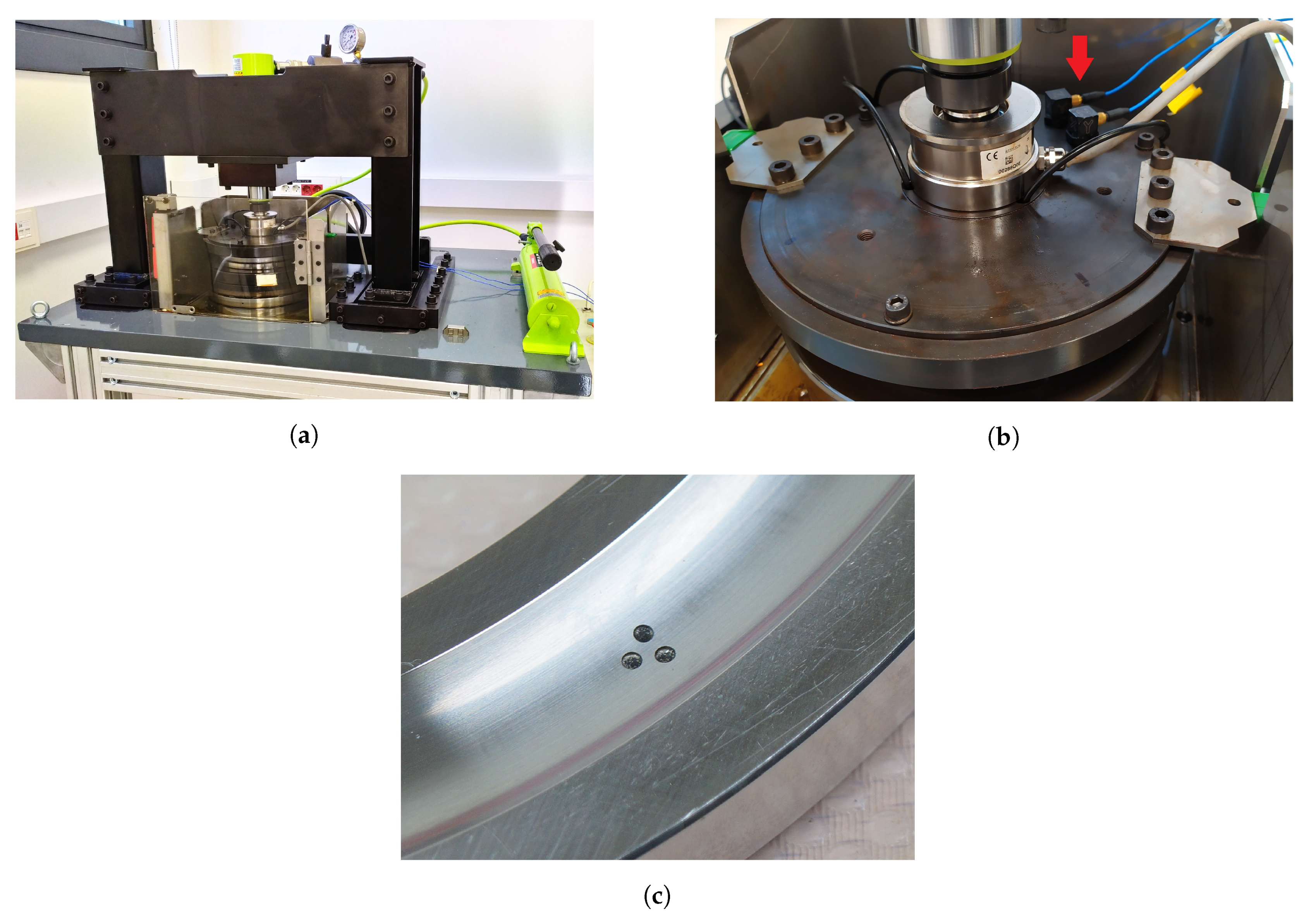
3. Experimental Set-Up

In this study, several thrust ball bearings in a test-rig oriented to reproduce rolling contact fatigue were used for experimental testing (Figure 1a). As this test-rig can operate at very low rotational speed condition (from 3 rpm) and high loads can be applied to the bearing [62], the configuration is in concordance to the conditions used in several and prominent publications found in the literature [33,63,64,65], and thus the configuration was appropriate for this study.

The installed bearings were FAG 51226 thrust ball bearings. For the experimental set-up, one bearing was used for each scenario—a healthy scenario (HS), damage 1 scenario (D1), and damage 2 scenario (D2). The faults from the damaged bearings D1 and D2 were artificially seeded to the shaft washers by electro-discharge machining before the tests, to reproduce one of the main faults in low-speed bearings [66]. The type and size of the damage seeded in the bearings were chosen after reviewing the several types of damage reported in the literature—natural damage [28], accelerated damage [67], and artificial damage [68]. Each damaged bearing had three circular damage of the same size that were equally spaced by 1 mm from each other (Figure 1c). D1 has circular damage with diameters of $1.5$ mm and for D2, 3 mm. All circular damage are $0.3$ mm deep.

The vibration signal data set used in this study was obtained by operating the bearings continuously at 5 rpm and 10 rpm over time, which were acquired with a 356A16 ICP acceleration sensor (PCB Piezoelectronics). The sensors were attached to the surface of the upper support disc (Figure 1b) by a wax adhesive. The raw data were acquired at $10.24$ $\mathrm{k}$$\mathrm{Hz}$ from the sensor using a data acquisition system from National Instruments (cDAQ 9174), and later, the raw data were processed as described in the following section.

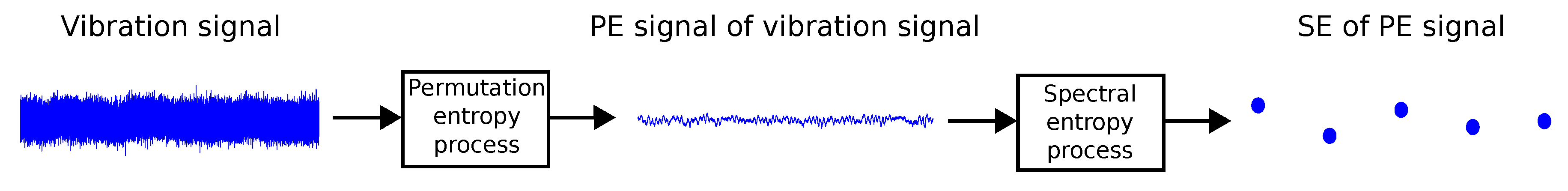
4. Methodology

According to the theory of rolling element bearings, once a bearing has incipient damage, several characteristic harmonics arise in the frequency spectrum [68]. The frequency and size of the harmonics are related to the damage size and type, respectively (the bigger the damage size, the greater the harmonic magnitude). This asseveration explains the application of the SE to the PE signal. When the original vibration signal is damaged, the PE signal can detect the damage, because of the changes in the fundamental harmonics of the signal. To quantify the trend and the harmonics, and hence the damage, SE is applied to the PE signal.

To analyze the raw vibration signals ${\left\{x_t\right\}}_{t=1,\dots ,T}$, the first step is calculating the PE signal ${\left\{p_t\right\}}_{t=1,\dots ,T^{\prime }}$, with $T^{\prime }=T-W_p$. To obtain $p_1$, Equation (9) is applied to $\{x_1,x_2\dots ,x_{W_p}\}$. The same step is then applied $\{x_2,x_3,\dots ,x_{W_p+1}\}$ for $p_2$. This process is continuously performed until the set $\{x_{T-W_p+1},\dots ,x_T\}$. This calculation has two main parameters: the window size $W_p$ and the permutation order $O_p$. For the $W_p$ selection, Figure 2 shows several PE signals calculated for a 30 s vibration signal (approximately five complete rotations) from a D2 bearing at 10 rpm as example. $W_p$ is different for each signal, with values from 128 to 16,384 samples (using powers of two for calculation purposes) and $O_p=3$. The results reveal that, for values lower than $W_p=2048$, unlike values greater than $W_p=2048$, a larger amount of noise and the loss of any representativeness of the original signal can be observed in the calculated signal.

The selection of the $O_p$ value is performed with several PE signals computed using a process similar to that used for $W_p$ selection. The calculation uses $O_p=\{3,4,5,6\}$, as $W_p$ covers less than $7!$ samples. The results have the same waveform, but the amplitude reduces for higher $O_p$ values (Figure 3). Because a higher value requires more computational effort and amplitude has no influence on the SE, the signal $O_p=3$ is employed to reduce computing time.

Figure 4 shows graphically the steps followed for the analysis of a vibration signal; they are summarized as follows:

• The raw vibration signal is used for the PE process. As a result, the PE signal is obtained from the PE process.
• The PE signal is later used by the SE process to calculate the SE value according to the rotation time.

The SE calculation of the PE signals is normalized to compare results [59]. For values close to 1, SE indicates uniform PSD of the analyzed signal. In contrast, values close to zero imply a concentration of the PSD in some harmonics of the frequency domain. Unlike that for PE, the SE calculation has no further parameters.

One last parameter to take into account is the elapsed time. As mentioned, the calculation is to be used in a CBM system, where incipient damage can take weeks, months, or even years to emerge. Incipient damage can be spotted anywhere on the bearing; therefore, for the entire bearing, the minimum time analyzed is the time needed for one rotation. For the case of 5 and 10 rpm, the bearing takes 12 s and 6 s for a full rotation. As the signals from the data set are 20 min long, there are approximately 100 rotations for the case of 5 rpm and 200 rotations for 10 rpm. The computation is performed to analyze the SE values calculated for one or more rotations, to integrate the results in a diagnostic model.

5. Results

This section shows the results obtained from the data set defined in Section 3 by application of the methodology described in Section 4. The computed values are summarized in Figure 5 and Figure 6 for 5 and 10 rpm, respectively.

Figure 5a shows the SE values for each rotation in HS, D1, and D2, along with their affine linear regression. The obtained results are in the band of 0.05 to 0.35, as the SE values are normalized. Figure 5a reveals a general pattern for each scenario, where the values for HS are on the top of the figure and the values for D2 are close to the bottom. The values for HS and D1 are significantly close in comparison to the values for D2, which are clearly separated to the aforementioned scenarios. In comparison to HS values, values for D1 and D2 are closer to 0, specially for the case with the bigger damage D2. The affine regresion for each data set can help to discern the difference among scenarios which are detected visually. From

Table 1. Linear regressions for all the scenarios at 5 rpm.

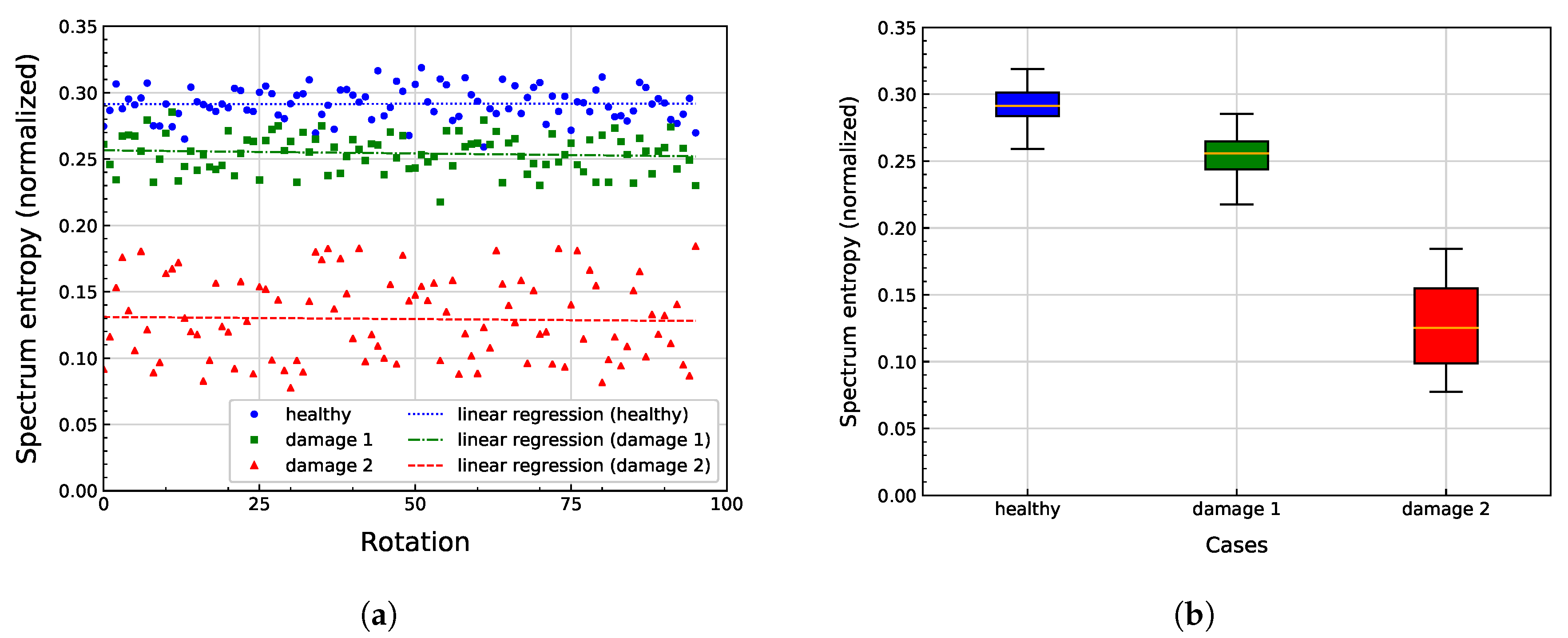
	Slope	y-intercept
healthy	−4.24 × 10−6	0.29
damage 1	−4.74 × 10−5	0.26
damage 2	−3.18 × 10−5	0.13

, the negative slope values reveal a very slow but steady decrease trend of the values through time. The y-intercept values expose the distance of each scenario trend to 0, where HS trend is the most distant and the D2 trend the closest one. For D1, the distance is slightly smaller in comparison to HS.

To better understand the obtained values in each scenario, a statistical summary is given by the boxplot in Figure 5b and the average $\overline{x}$, median Md, and standard deviation s values for each scenario in

Table 2. Statistical data for all the scenarios at 5 rpm.

	$\overline{\mathit{x}}$	Md	s
healthy	0.292	0.291	0.012
damage 1	0.254	0.256	0.014
damage 2	0.129	0.125	0.031

. From Figure 5b, the lowest average and median are from D2 and the highest are from HS. The average value of D1 is higher in comparison to D2 and closer to HS, which is consistent with the visual examination of Figure 5a. The boxplot shows an overlay of the values from D1 and HS. In specific, the first two quartiles of HS are overlapped to the calculated values from D1. The standard deviation for D2 is specially higher in comparison to D1 and HS, as seen in Figure 5b. Overall, and considering as reference the values of HS, the average values decrease for D1 (13%) and D2 (56%). For the median, a decrease is also notable for D1 (12%) and D2 (57%).

Results obtained for data at 10 rpm can be seen in Figure 6a, where the SE values for HS, D1, and D2, along with their affine linear regression are shown. The figure shows values in the band of 0.1 to 0.3 for the normalized value of SE. In general, the values corresponding to HS are higher than those of the bearings with damage. The trend for the D1 and D2 values is significantly below the value trend for the HS bearing, which is lower when the size of circular damage is higher. Although the values from D1 can be seen as overlapping the HS values, the affine linear regression for each set of data have different slope and y-intercept values (

Table 3. Linear regressions for all the scenarios at 10 rpm.

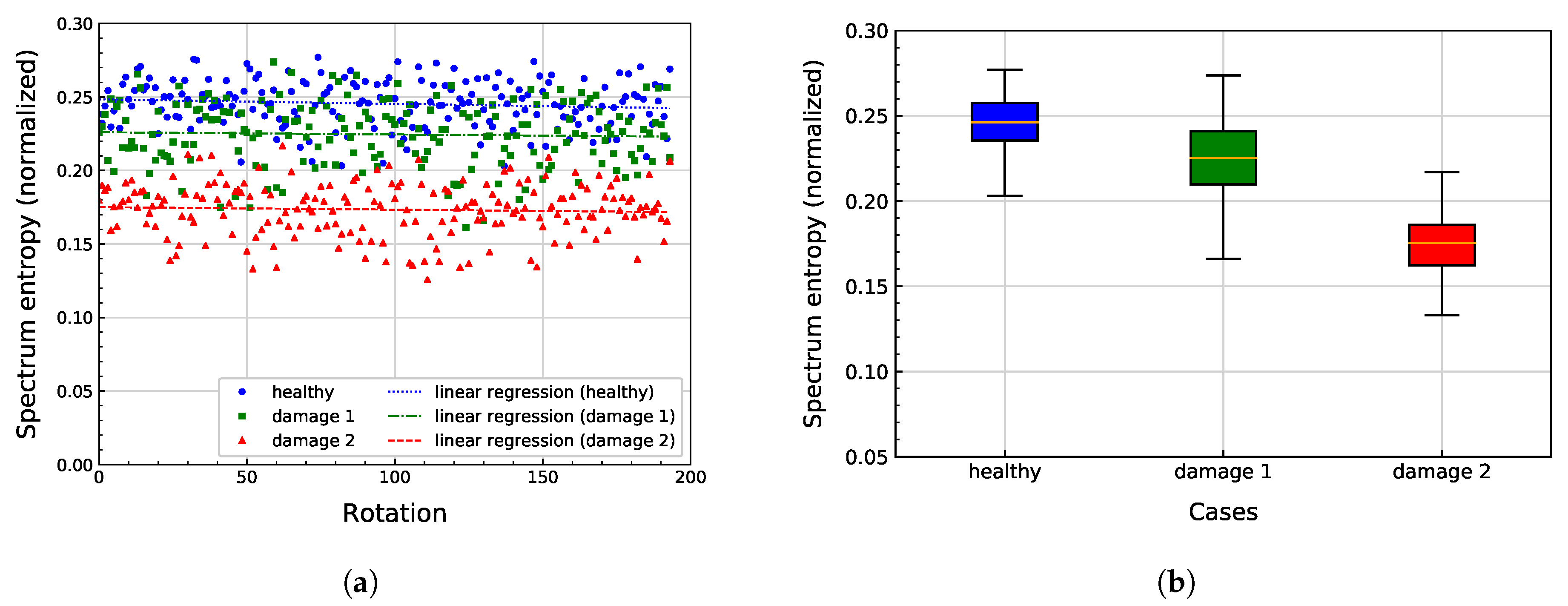
	Slope	y-intercept
healthy	−3.05 × 10−5	0.25
damage 1	−1.51 × 10−5	0.23
damage 2	−1.71 × 10−5	0.18

). In contrast, the differences between data from HS and D2 are easy to observe in the figure. The linear regression highlights the disparities among the scenarios. As Table 3 shows, the slopes are negative. The y-intercept value for HS is the largest of all the values for the three scenarios, and the lowest value is for the D2 scenario.

A statistical summary of the data from each scenario is shown in Figure 6b. The average $\overline{x}$, median Md, and standard deviation s of each scenario are shown in

Table 4. Statistical data for all the scenarios at 10 rpm.

	$\overline{\mathit{x}}$	Md	s
healthy	0.245	0.246	0.016
damage 1	0.225	0.225	0.022
damage 2	0.173	0.175	0.018

. From Figure 6b, HS has the highest average value and median. As D1 and D2 have lower values of $\overline{x}$ in comparison with HS, $\overline{x}$ is lower when seeded damage exists. This situation also occurs for the median, which has a higher value in HS, but is lower for D1 and D2. The standard deviations for HS and D2 are similar, but for D1, the standard deviation is significantly higher than those for HS and D2. This value corresponds to the observed trend for Figure 6a. The box plot shows an overlay of the values from HS and D1. In particular, the last three quartiles of D1 are overlapped with the values from the SE calculation for the HS. Overall, and considering as reference the values of HS, the average value for D1 decrement 8% and D2 almost 30%. For the median, D1 decrement almost 9% and D2 29%.

The results in Figure 5 and Figure 6 indicate that the calculated SE of the PE signal can discriminate between a healthy bearing and a bearing with incipient damage from the point of view of a classification problem. This might be since the energy released by a damaged bearing, which is related to the operating speed of the bearing, the size of the damage, and the magnitude of the harmonics. The quantity of the released energy (detected as vibration by the sensor) for low-speed bearings is reflected in the magnitude of the produced harmonics, which are in general small enough to be confused as noise in the signal. Therefore, as the released energy for incipient damage is not high enough, it cannot be distinguished from the noise in the signal. Nevertheless, the released energy produces harmonics. The proposed method hardly recognizes the trends from the energy release caused by the incipient damage, allowing slight detection exposed to results from both rotational speeds.

For the case of a healthy bearing and established damage, an expected result would be a bigger difference among scenarios for higher than lower rpm (a higher rotational speed means higher energy release). However, results show a bigger difference between HS and D2 for data at 5 rpm in comparison to 10 rpm. As reviewed in the literature, not all indicators are useful for all rotational speed range. From this perspective, the proposed method might have a better behavior for rotational speed closer to 1, as the numerical difference between a healthy and established damage scenario is bigger for the lower rotational speed. Further studies could confirm this assumption.

The energy quantity from the established damage is large enough to be distinguishable from healthy and incipient damage, as the results reveal. For a better awareness of the method and its behavior under several types of damage and rotational speed, so that a robust method for the diagnosis of bearing damage can be developed, a variety of damage types and rotational speed should be studied.

6. Conclusions

In this paper, PE and SE are introduced for the analysis of vibration signals belonging to scenarios with very low-speed bearings. The current study demonstrates the existence of a relationship between the calculated entropy-based indicator and the presence of damage on a bearing at 5 rpm and 10 rpm without the need of previous noise filtering. Specifically, the values of the entropy-based indicator are reduced as the damage size increases. The decrement of the values calculated from a damaged scenario can be up to 57% when the median value is compared to a healthy scenario and 55% for the average value.

To apply the proposed entropy-based indicator in a real scenario, several conditions should be taken into account. In this study, the proposed entropy-based indicator is applied to a controlled scenario, where the speed and the forces on the bearing are always continuous. A subsequent study can consider variable forces to the bearing, as the wind speed through the day. The same condition can be implemented for the speed with different speed values to observe the capability of the proposed indicator near to 1 rpm. The use of a back and forth rotation condition to replicate the movement of a real pitch bearing, hence a more realistic scenario, can also be considered in further studies.

The investigated scenarios included only two damage sizes located in one race of each bearing. Thus, the possible scenarios that could be utilized to study the performance of the proposed entropy-based indicator were limited. Further studies can focus on several types and combinations of damage, such as ball, or cage damage, to address the fault identification problem. The inclusion of several damage sizes (smaller and larger than the ones used) in race, ball or cage can also contribute to dealing with the quantification problem. A different scenario to consider is a naturally induced damage to the bearing, which increases in size over time. The mentioned scenarios could help researchers to identify the properties and limitations of the methodology presented and its use in CBM. Finally, the proposed entropy-based indicator can be used for the design of diagnosis models based on artificial intelligence for a subsequent stage in real CBM systems.

References

- Komusanac, I.; Fraile, D.; Brindley, G. Wind Energy in Europe in 2018; Technical Report; Wind Europe: Brussels, Belgium, 2019. [Google Scholar]
- Walsh, C.; Ramírez, L.; Fraile, D.; Brindley, G. Wind Energy in Europe in 2019; Technical Report; Wind Europe: Brussels, Belgium, 2020. [Google Scholar]
- IRENA. Future of Wind: Deployment, Investment, Technology, Grid Integration and Socio-Economic Aspects (A Global Energy Transformation Paper); Technical Report; International Renewable Energy Agency: Abu Dhabi, UAE, 2019. [Google Scholar]
- IRENA. Renewable Energy Cost Analysis—Wind Power; Technical Report; International Renewable Energy Agency: Abu Dhabi, UAE, 2012. [Google Scholar]
- IRENA. Floating Foundations: A Game Changer for Offshore Wind Power; Technical Report; International Renewable Energy Agency: Abu Dhabi, UAE, 2016. [Google Scholar]
- Lynn, P. Onshore and Offshore Wind Energy: An Introduction, 1st ed.; John Wiley & Sons Ltd.: West Sussex, UK, 2011. [Google Scholar]
- Tchakoua, P.; Wamkeue, R.; Ouhrouche, M.; Slaoui-Hasnaoui, F.; Tameghe, T.A.; Ekemb, G. Wind Turbine Condition Monitoring: State-of-the-Art Review, New Trends, and Future Challenges. Energies 2014, 7, 2595–2630. [Google Scholar] [CrossRef] [Green Version]
- Kania, L.; Krynke, M.; Mazanek, E. A Catalogue Capacity of Slewing Bearings. Mech. Mach. Theory 2012, 58, 29–45. [Google Scholar] [CrossRef]
- Ossai, C.I.; Boswell, B.; Davies, I.J. A Markovian Approach for Modelling the Effects of Maintenance on Downtime and Failure Risk of Wind Turbine Components. Renew. Energy 2016, 96, 775–783. [Google Scholar] [CrossRef]
- Stamboliska, Z.; Rusiński, E.; Moczko, P. Condition Monitoring Considerations for Low-Speed Machines. In Proactive Condition Monitoring of Low-Speed Machines; Springer International Publishing: Cham, Switzerland, 2015; pp. 35–52. [Google Scholar]
- Wang, F.; Liu, C.; Su, W.; Xue, Z.; Li, H.; Han, Q. Condition Monitoring and Fault Diagnosis Methods for Low-Speed and Heavy-Load Slewing Bearings: A Literature Review. J. Vibroeng. 2017, 19, 3429–3444. [Google Scholar] [CrossRef]
- Liu, Z.; Zhang, L. A Review of Failure Modes, Condition Monitoring and Fault Diagnosis Methods for Large-Scale Wind Turbine Bearings. Measurement 2020, 149, 107002. [Google Scholar] [CrossRef]
- Sandoval, D.; Leturiondo, U.; Pozo, F.; Vidal, Y.; Salgado, O. Revisión de las técnicas de monitorización del estado de los rodamientos de las palas de los aerogeneradores. DYNA 2019, 94, 636–642. [Google Scholar] [CrossRef]
- Sandoval, D.; Leturiondo, U.; Pozo, F.; Vidal, Y.; Salgado, O. Trends in Condition Monitoring for Pitch Bearings. In Proceedings of the 16th International Conference on Condition Monitoring and Asset Management, CM, Glasgow, UK, 25–27 June 2019. [Google Scholar] [CrossRef]
- Elforjani, M.; Mba, D. Monitoring the Onset and Propagation of Natural Degradation Process in a Slow Speed Rolling Element Bearing With Acoustic Emission. J. Vib. Acoust. 2008, 130, 041013. [Google Scholar] [CrossRef]
- Omoregbee, O.; Heyns, P. Low Speed Rolling Bearing Diagnostics Using Acoustic Emission and Higher Order Statistics Techniques. J. Mech. Eng. Res. Dev. 2018, 41, 18–23. [Google Scholar] [CrossRef]
- He, Y.; Zhang, X.; Friswell, M.I. Defect Diagnosis for Rolling Element Bearings Using Acoustic Emission. J. Vib. Acoust. 2009, 131, 061012. [Google Scholar] [CrossRef] [Green Version]
- Elforjani, M.; Mba, D. Accelerated Natural Fault Diagnosis in Slow Speed Bearings with Acoustic Emission. Eng. Fract. Mech. 2010, 77, 112–127. [Google Scholar] [CrossRef]
- He, Y.; Zhang, X. Approximate Entropy Analysis of the Acoustic Emission From Defects in Rolling Element Bearings. J. Vib. Acoust. 2012, 134, 061012. [Google Scholar] [CrossRef]
- Caesarendra, W.; Kosasih, B.; Tieu, A.K.; Zhu, H.; Moodie, C.A.S.; Zhu, Q. Acoustic Emission-Based Condition Monitoring Methods: Review and Application for Low Speed Slew Bearing. Mech. Syst. Signal Process. Dev. 2016, 72–73, 134–159. [Google Scholar] [CrossRef]
- Caesarendra, W.; Kosasih, B.; Tieu, K.; Moodie, C. An Application of Nonlinear Feature Extraction—A Case Study for Low Speed Slewing Bearing Condition Monitoring and Prognosis. In Proceedings of the 2013 IEEE/ASME International Conference on Advanced Intelligent Mechatronics: Mechatronics for Human Wellbeing, AIM, Wollongong, NSW, Australia, 9–12 July 2013; pp. 1713–1718. [Google Scholar] [CrossRef] [Green Version]
- Rojas, A.; Nandi, A.K. Detection and Classification of Rolling-Element Bearing Faults Using Support Vector Machines. In Proceedings of the 2005 IEEE Workshop on Machine Learning for Signal Processing, Mystic, CT, USA, 28–28 September 2005; pp. 153–158. [Google Scholar] [CrossRef]
- Caesarendra, W.; Tjahjowidodo, T. A Review of Feature Extraction Methods in Vibration-Based Condition Monitoring and Its Application for Degradation Trend Estimation of Low-Speed Slew Bearing. Machines 2017, 5, 21. [Google Scholar] [CrossRef]
- Moodie, C. An Investigation into the Condition Monitoring of Large Slow Speed Slew Bearings. In University of Wollongong Thesis Collection 1954–2016: Wollongong; University of Wollongong: Wollongong, Australia, 2009. [Google Scholar]
- Caesarendra, W.; Tjahjowidodo, T.; Kosasih, B.; Tieu, A. Integrated Condition Monitoring and Prognosis Method for Incipient Defect Detection and Remaining Life Prediction of Low Speed Slew Bearings. Machines 2017, 5, 11. [Google Scholar] [CrossRef] [Green Version]
- Jiao, Y.; Li, G.; Wu, Z.; Geng, H.; Zhang, J.; Cheng, L. Fault Analysis for Low-Speed Heavy-Duty Crane Slewing Bearing Based on Wavelet Energy Spectrum Coefficient. In Advances in Acoustic Emission Technology; Shen, G., Wu, Z., Zhang, J., Eds.; Springer International Publishing: Cham, Switzerlaned, 2017; pp. 63–74. [Google Scholar]
- Mishra, C.; Samantaray, A.; Chakraborty, G. Rolling Element Bearing Fault Diagnosis under Slow Speed Operation Using Wavelet De-Noising. Meas. J. Int. Meas. Confed. 2017, 103, 77–86. [Google Scholar] [CrossRef]
- Liu, Z.; Zhang, L.; Carrasco, J. Vibration Analysis for Large-Scale Wind Turbine Blade Bearing Fault Detection with an Empirical Wavelet Thresholding Method. Renew. Energy 2020, 146, 99–110. [Google Scholar] [CrossRef]
- Yu, K.; Lin, T.R.; Tan, J.; Ma, H. An Adaptive Sensitive Frequency Band Selection Method for Empirical Wavelet Transform and Its Application in Bearing Fault Diagnosis. Measurement 2019, 134, 375–384. [Google Scholar] [CrossRef]
- Wang, S.; Niu, P.; Guo, Y.; Wang, F.; Li, W.; Shi, H.; Han, S. Early Diagnosis of Bearing Faults Using Decomposition and Reconstruction Stochastic Resonance System. Measurement 2020, 158, 107709. [Google Scholar] [CrossRef]
- Caesarendra, W.; Kosasih, P.; Tieu, A.; Moodie, C.; Choi, B.K. Condition Monitoring of Naturally Damaged Slow Speed Slewing Bearing Based on Ensemble Empirical Mode Decomposition. J. Mech. Sci. Technol. 2013, 27, 2253–2262. [Google Scholar] [CrossRef]
- Bao, W.; Miao, X.; Wang, H.; Yang, G.; Zhang, H. Remaining Useful Life Assessment of Slewing Bearing Based on Spatial-Temporal Sequence. IEEE Access 2020, 8, 9739–9750. [Google Scholar] [CrossRef]
- Han, T.; Liu, Q.; Zhang, L.; Tan, A. Fault Feature Extraction of Low Speed Roller Bearing Based on Teager Energy Operator and CEEMD. Meas. J. Int. Meas. Confed. 2019, 138, 400–408. [Google Scholar] [CrossRef]
- Richman, J.S.; Moorman, J.R. Physiological Time-Series Analysis Using Approximate Entropy and Sample Entropy. Am. J. Physiol. Heart Circ. Physiol. 2000, 278, H2039–H2049. [Google Scholar] [CrossRef] [PubMed] [Green Version]
- Henry, M.; Judge, G. Permutation Entropy and Information Recovery in Nonlinear Dynamic Economic Time Series. Econometrics 2019, 7, 10. [Google Scholar] [CrossRef] [Green Version]
- Shang, Y.; Lu, G.; Kang, Y.; Zhou, Z.; Duan, B.; Zhang, C. A Multifault Diagnosis Method Based on Modified Sample Entropy for Lithium-Ion Battery Strings. J. Power Sources 2020, 446, 227275. [Google Scholar] [CrossRef]
- Yan, R.; Gao, R.X. Approximate Entropy as a Diagnostic Tool for Machine Health Monitoring. Mech. Syst. Signal Process. 2007, 21, 824–839. [Google Scholar] [CrossRef]
- Xu, Y.; Chen, R.; Li, Y.; Zhang, P.; Yang, J.; Zhao, X.; Liu, M.; Wu, D. Multispectral Image Segmentation Based on a Fuzzy Clustering Algorithm Combined with Tsallis Entropy and a Gaussian Mixture Model. Remote Sens. 2019, 11, 2772. [Google Scholar] [CrossRef] [Green Version]
- Xue, W.; Dai, X.; Zhu, J.; Luo, Y.; Yang, Y. A Noise Suppression Method of Ground Penetrating Radar Based on EEMD and Permutation Entropy. IEEE Geosci. Remote Sens. Lett. 2019, 16, 1625–1629. [Google Scholar] [CrossRef]
- Fei, C.W.; Choy, Y.S.; Bai, G.C.; Tang, W.Z. Multi Feature Entropy Distance Approach with Vibration and Acoustic Emission Signals for Process Feature Recognition of Rolling Element Bearing Faults. Struct. Health Monit. 2017, 17, 156–168. [Google Scholar] [CrossRef]
- Gu, R.; Chen, J.; Hong, R.; Wang, H.; Wu, W. Incipient Fault Diagnosis of Rolling Bearings Based on Adaptive Variational Mode Decomposition and Teager Energy Operator. Measurement 2020, 149, 106941. [Google Scholar] [CrossRef]
- Zhang, J.; Zhao, Y.; Li, X.; Liu, M. Bearing Fault Diagnosis with Kernel Sparse Representation Classification Based on Adaptive Local Iterative Filtering-Enhanced Multiscale Entropy Features. Math. Probl. Eng. 2019, 2019, 7905674. [Google Scholar] [CrossRef] [Green Version]
- Zhao, D.; Liu, S.; Gu, D.; Sun, X.; Wang, L.; Wei, Y.; Zhang, H. Improved Multi-Scale Entropy and It’s Application in Rolling Bearing Fault Feature Extraction. Measurement 2020, 152, 107361. [Google Scholar] [CrossRef]
- Yang, C.; Jia, M. Health Condition Identification for Rolling Bearing Based on Hierarchical Multiscale Symbolic Dynamic Entropy and Least Squares Support Tensor Machine–Based Binary Tree. Struct. Health Monit. 2020. [Google Scholar] [CrossRef]
- Huo, Z.; Zhang, Y.; Jombo, G.; Shu, L. Adaptive Multiscale Weighted Permutation Entropy for Rolling Bearing Fault Diagnosis. IEEE Access 2020, 8, 87529–87540. [Google Scholar] [CrossRef]
- Fu, W.; Shao, K.; Tan, J.; Wang, K. Fault Diagnosis for Rolling Bearings Based on Composite Multiscale Fine-Sorted Dispersion Entropy and SVM With Hybrid Mutation SCA-HHO Algorithm Optimization. IEEE Access 2020, 8, 13086–13104. [Google Scholar] [CrossRef]
- Wang, H.; Du, W. Feature Extraction of Latent Fault Components of Rolling Bearing Based on Self-Learned Sparse Atomics and Frequency Band Entropy. J. Vib. Control 2020. [Google Scholar] [CrossRef]
- Wang, F.; Zhang, Y.; Zhang, B.; Su, W. Application of Wavelet Packet Sample Entropy in the Forecast of Rolling Element Bearing Fault Trend. In Proceedings of the 2011 International Conference on Multimedia and Signal Processing, Toronto, ON, Canada, 27–28 April 2011; Volume 2, pp. 12–16. [Google Scholar] [CrossRef]
- Qin, X.; Li, Q.; Dong, X.; Lv, S. The Fault Diagnosis of Rolling Bearing Based on Ensemble Empirical Mode Decomposition and Random Forest. 2017. Available online: https://www.hindawi.com/journals/sv/2017/2623081/ (accessed on 26 June 2020).
- Li, H.; Liu, T.; Wu, X.; Chen, Q. Enhanced Frequency Band Entropy Method for Fault Feature Extraction of Rolling Element Bearings. IEEE Trans. Ind. Inform. 2020, 16, 5780–5791. [Google Scholar] [CrossRef]
- Lu, C.; Chen, J.; Hong, R.; Feng, Y.; Li, Y. Degradation Trend Estimation of Slewing Bearing Based on LSSVM Model. Mech. Syst. Signal Process. 2016, 76–77, 353–366. [Google Scholar] [CrossRef]
- Shannon, C.E. A Mathematical Theory of Communication. Bell Syst. Tech. J. 1948, 27, 379–423. [Google Scholar] [CrossRef] [Green Version]
- Goodfellow, I.; Bengio, Y.; Courville, A. Deep Learning; MIT Press: Cambridge, UK, 2016. [Google Scholar]
- Rostaghi, M.; Azami, H. Dispersion Entropy: A Measure for Time-Series Analysis. IEEE Signal Process. Lett. 2016, 23, 610–614. [Google Scholar] [CrossRef]
- Gorobets, A.Y.; Berdyugina, S.V. Stochastic Entropy Production in the Quite Sun Magnetic Fields. Mon. Not. R. Astron. Soc. Lett. 2018, 483, L69–L74. [Google Scholar] [CrossRef]
- Bandt, C.; Pompe, B. Permutation Entropy: A Natural Complexity Measure for Time Series. Phys. Rev. Lett. 2002, 88, 174102. [Google Scholar] [CrossRef]
- Fouda, J.S.A.E.; Koepf, W.; Jacquir, S. The Ordinal Kolmogorov-Sinai Entropy: A Generalized Approximation. Commun. Nonlinear Sci. Numer. Simul. 2017, 46, 103–115. [Google Scholar] [CrossRef]
- Powell, G.E.; Percival, I.C. A Spectral Entropy Method for Distinguishing Regular and Irregular Motion of Hamiltonian Systems. J. Phys. A Math. Gen. 1979, 12, 2053–2071. [Google Scholar] [CrossRef]
- Inouye, T.; Shinosaki, K.; Sakamoto, H.; Toi, S.; Ukai, S.; Iyama, A.; Katsuda, Y.; Hirano, M. Quantification of EEG Irregularity by Use of the Entropy of the Power Spectrum. Electroencephalogr. Clin. Neurophysiol. 1991, 79, 204–210. [Google Scholar] [CrossRef]
- Abásolo, D.; Hornero, R.; Espino, P.; Álvarez, D.; Poza, J. Entropy Analysis of the EEG Background Activity in Alzheimer\textquotesingles Disease Patients. Physiol. Meas. 2006, 27, 241–253. [Google Scholar] [CrossRef] [Green Version]
- Pan, Y.N.; Chen, J.; Li, X.L. Spectral Entropy: A Complementary Index for Rolling Element Bearing Performance Degradation Assessment. Proc. Inst. Mech. Eng. Part C J. Mech. Eng. Sci. 2008. [Google Scholar] [CrossRef]
- Harris, T.; Rumbarger, J.H.; Butterfield, C.P. Wind Turbine Design Guideline DG03: Yaw and Pitch Rolling Bearing Life; Technical Report; National Renewable Energy Laboratory: Golden, CO, USA, 2009. [CrossRef] [Green Version]
- Caesarendra, W.; Pratama, M.; Tjahjowidodo, T.; Tieud, K.; Kosasih, B. Parsimonious Network Based on Fuzzy Inference System (PANFIS) for Time Series Feature Prediction of Low Speed Slew Bearing Prognosis. Appl. Sci. 2018, 8, 2656. [Google Scholar] [CrossRef] [Green Version]
- Wang, S.; Chen, J.; Wang, H.; Zhang, D. Degradation Evaluation of Slewing Bearing Using HMM and Improved GRU. Measurement 2019. [Google Scholar] [CrossRef]
- Bao, W.; Wang, H.; Chen, J.; Zhang, B.; Ding, P.; Wu, J.; He, P. Life Prediction of Slewing Bearing Based on Isometric Mapping and Fuzzy Support Vector Regression. Trans. Inst. Meas. Control 2019. [Google Scholar] [CrossRef]
- Liu, C.; Wang, F. A Review of Current Condition Monitoring and Fault Diagnosis Methods for Low-Speed and Heavy-Load Slewing Bearings. In Proceedings of the 2017 9th International Conference on Modelling, Identification and Control, ICMIC, Kunming, China, 10–12 July 2017; Volume 2018, pp. 104–109. [Google Scholar] [CrossRef]
- Caesarendra, W.; Kosasih, B.; Tieu, A.; Moodie, C. Circular Domain Features Based Condition Monitoring for Low Speed Slewing Bearing. Mech. Syst. Signal Process. 2014, 45, 114–138. [Google Scholar] [CrossRef] [Green Version]
- Randall, R.B.; Antoni, J. Rolling Element Bearing Diagnostics—A Tutorial. Mech. Syst. Signal Process. 2011, 25, 485–520. [Google Scholar] [CrossRef]