Machine Learning Applied to Diagnosis of Human Diseases: A Systematic Review

Abstract

Human healthcare is one of the most important topics for society. It tries to find the correct effective and robust disease detection as soon as possible to patients receipt the appropriate cares. Because this detection is often a difficult task, it becomes necessary medicine field searches support from other fields such as statistics and computer science. These disciplines are facing the challenge of exploring new techniques, going beyond the traditional ones. The large number of techniques that are emerging makes it necessary to provide a comprehensive overview that avoids very particular aspects. To this end, we propose a systematic review dealing with the Machine Learning applied to the diagnosis of human diseases. This review focuses on modern techniques related to the development of Machine Learning applied to diagnosis of human diseases in the medical field, in order to discover interesting patterns, making non-trivial predictions and useful in decision-making. In this way, this work can help researchers to discover and, if necessary, determine the applicability of the machine learning techniques in their particular specialties. We provide some examples of the algorithms used in medicine, analysing some trends that are focused on the goal searched, the algorithm used, and the area of applications. We detail the advantages and disadvantages of each technique to help choose the most appropriate in each real-life situation, as several authors have reported. The authors searched Scopus, Journal Citation Reports (JCR), Google Scholar, and MedLine databases from the last decades (from 1980s approximately) up to the present, with English language restrictions, for studies according to the objectives mentioned above. Based on a protocol for data extraction defined and evaluated by all authors using PRISMA methodology, 141 papers were included in this advanced review.

1. Introduction

Healthcare is one of the most urgent matters in human societies, as the life quality of citizens directly depends on it [1]. However, the healthcare sector is highly heterogeneous, widely distributed and fragmented. From the clinical perspective, delivering appropriate patient care requires access to relevant patient information, which is seldom available where and when it is needed [2]. Additionally, the wide variation in test-ordering for diagnostic purposes suggests the requirement of sufficient and appropriate test set [3,4]. Smellie et al. [5] extended this argument by suggesting that the large differences observed in general practice pathology requesting result mostly from individual variation in clinical practice and are, therefore, potentially susceptible to change through more consistent and better informed decision-making for doctors [6].

Hence, medical data often consist of a large set of heterogeneous variables, collected from different sources, such as demographics, disease history, medication, allergies, biomarkers, medical images, or genetic markers, each of which offer a different partial view on a patient’s state. Moreover, statistical properties among the aforementioned sources are inherently different. When researchers and practitioners analyse such data, they are confronted with two problems: the curse of dimensionality (the feature space is increasing exponentially in the number of dimensions and the number of samples), and the heterogeneity in feature sources and statistical properties [7]. These factors provoke delays and inaccuracy in the disease detection and, consequently, patients could not receive the appropriate cares [8]. Thus, there is a clear need for an effective and robust methodology that allows for the early disease detection and it can be used by doctors as a help for decision-making [9]. Therefore, medical, computational, and statistical fields are facing a challenge of exploring new techniques for modelling the prognosis and diagnosis of diseases, since traditional paradigms fail in the treatment of all this information [10]. This requirement is quite related to the evolutions in other domains, such as Big Data (BD), Data Mining (DM), or Artificial Intelligence (AI).

As the amount of medical data being digitally collected and stored is vast and expanding quickly, the science of data management and analysis is also advancing to convert this vast resource into information and knowledge that helps them achieve their objectives. The term BD is used to describe this evolving technology [11]. Subsequently, BD started with large-volume, heterogeneous, autonomous sources with distributed and decentralised control, and it seeks to explore complex and evolving relationships among data [12].

BD is a subset of DM, also known as knowledge discovery in databases. DM is the process of discovering interesting patterns in databases that are meaningful in decision-making and which lead to some advantage. Useful patterns allow us to make non-trivial predictions on new data and they help to explain something about the data [13]. However, finding these patterns is not an easy task. To this end, it is necessary to use advanced techniques for describing these structural patterns in data. Most of these techniques were developed within a field that is known as AI.

AI is a part of computer science that aims to make computers more intelligent. One of the basic requirements for any intelligent behaviour is learning. Currently, most researchers agree that there is no intelligence without learning. A learning problem can be defined as the difficulty of improving some measure when executing some tasks, through some type of training experience. In turn, within AI, Machine Learning (ML) emerged as a method of choice for developing algorithms to analyse datasets [14].

Today, ML provides several indispensable tools for intelligent data analysis. Additionally, its technology is currently well suited for analysing medical data and, in particular, there is a wide range of works done in medical diagnosis in small-specialised diagnostic problems [15], where initial applications of ML were pointed out. For example, ML classifiers have been successfully applied to distinguish between healthy and Parkinson patients [16], which is a useful tool in clinical diagnosis. Indeed, most ML algorithms work very well on a wide variety of important problems. However, they have not succeeded in solving the main problems in AI when they become exceedingly difficult and the number in the data is high (the curse of dimensionality). In these cases, BD technology is necessary. Thus, Deep Learning (DL) arose as a specific kind of ML. Hence, the development of DL was motivated and designed to overcome the failure of traditional algorithms to work with high-dimensional data, and learn complex functions in high-dimensional spaces [17].

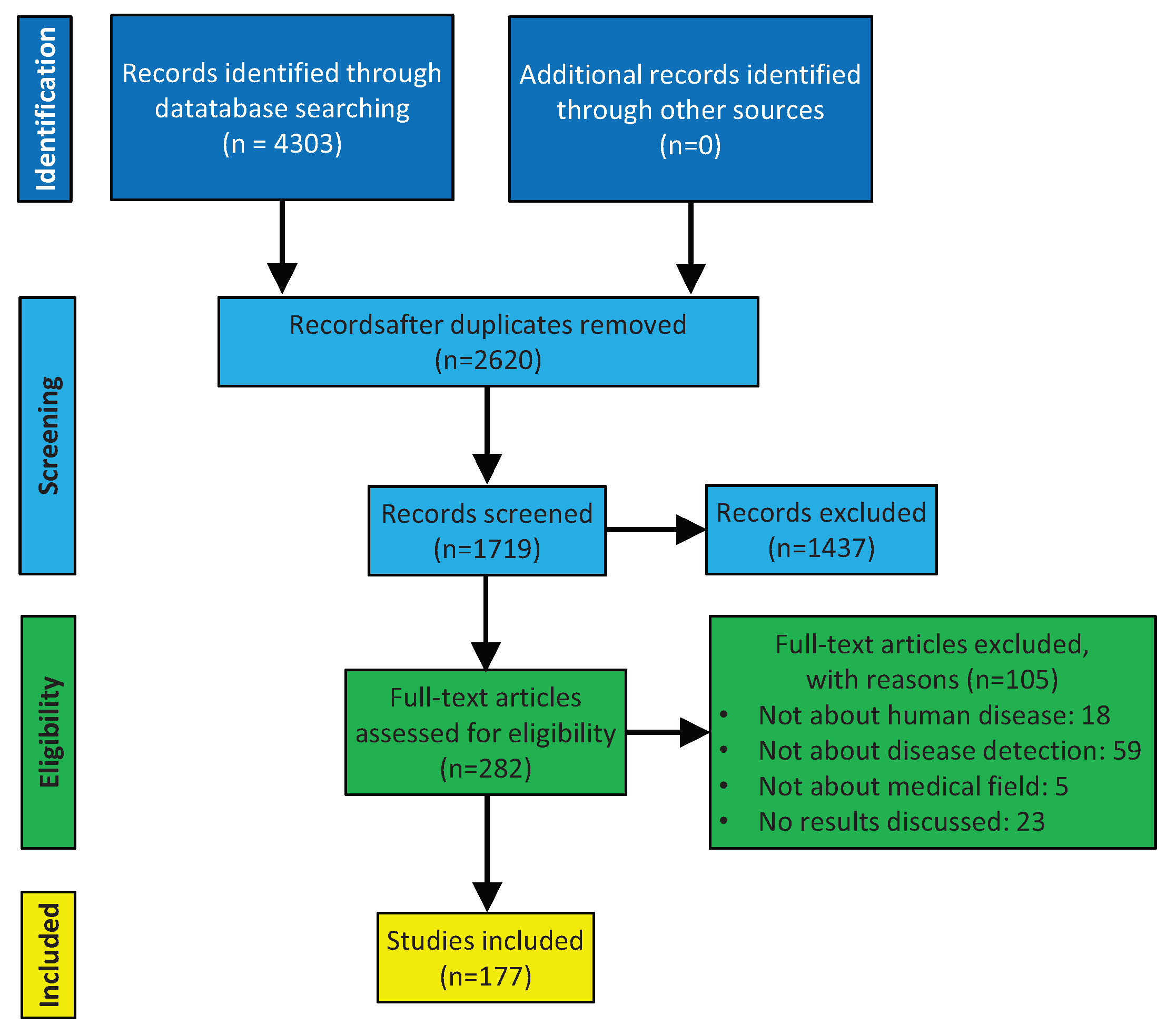
2. Methods

2.1. Data Sources

Based on the methodology of a systematic review [18], we systematically searched in literature databases, such as Scopus, Journal Citation Reports (JCR), Google Scholar, and MedLine from the last decades (from 1980s approximately) up to the present, with English language restrictions, for studies within the scope of AI, BD, DL, DM, and ML applied to diagnosis of human diseases in the medical field. As a result, we perform a sweep for all medical field, trying to maximise the application and techniques applied within medical field, obtaining a representative systematic review.

2.2. Data Extraction

A protocol for data extraction was defined and evaluated by all authors. The following inclusion criteria were used: studies with key words, such as Human Disease, Metabolic Disease, Cancer, Parkinson’s Disease, Alzheimer’s Disease, Heart Disease, Hepatic Disease, Infectious Disease, or Renal Disease; belonging to the thematic areas Data Mining, Artificial Intelligence, Big Data, Deep Learning, and Machine Learning; the document types as Indexed Journal Paper, Book, Book Chapter, and Conference Paper. Moreover, the following exclusion criteria were also used: not among the years 2008–2018, not belonging to the sub areas Data Mining, Artificial Intelligence, Big Data, Deep Learning, or Machine Learning; not Indexed Journal Paper, Book, Book Chapter, or Conference Paper as source type and not English language; topic addressed in other studies; not conclusive; not fully solved; nor with a tangential, not central, interest for the systematic review aims. Finally, some studies that were not between 2008 and 2018 were added to the outcome, as they contained relevant topics with a high citation index.

One researcher (NCC) extracted data, which were checked independently by other ones (JLCS, JAGP, JMGP, and MLPL). In case of unsure, the full text was retrieved. In case of disagreement about the application of the selection criteria, the case was discussed with reference to the protocol criteria and, if needed, the full paper was retrieved.

To determine the estimates, each study contributed with only one estimate. Whenever a study generated multiple estimates according to different diagnostic or methodological definitions, one estimate was selected according to a previously defined protocol. This protocol ensured that data on each subject were only extracted once. In case a study published in different dates, the extracted study was the last one. The quality of the papers included is endorsed by the exhaustive review process followed by the journals from the selected literature databases.

2.3. Data Analyses

The content of this paper deals with a systematic review, not in a meta-analysis of the state of the art related to the intelligent data analysis in the medical field. Nevertheless, it does not deepen into the details regarded to the results obtained in each case of study. Hence, data analysis techniques are not applicable in this case.

3. Results

Of 4303 citations, we included 177 papers that met the inclusion criteria. Figure 1 shows our search, selection process, and the reasons for their exclusion. Thus, this Section provides a summary of the 177 studies reviewed in this paper necessaries for understanding the intelligent data analysis performed in the medical field.

3.1. Machine Learning Principles

Every learning process, deep or not, consists of two phases: the estimation of unknown dependencies in a system from a given data set (input) and the use of estimated dependencies to predict new outputs of the system. In this Subsection, we analyse the most common techniques used in both phases.

3.1.1. Input. Definition and Methods

The input of a ML process is a set of instances. These instances are the things that can be classified, associated, or clustered. Each instance is an individual, i.e., independent example of the concept that must be learned. Additionally, each one is characterised by the values of a set of predetermined attributes. Each dataset is represented as a matrix of instances versus attributes, which, in database terms, is a flat file (single relation) [13]. Kourou et al. [19] defined the main common learning methods as unsupervised learning and supervised learning.

In unsupervised learning, non-labelled examples are provided and there is no notion of the output along the learning process. The aim in this kind of learning is to explore data by the end of finding different categories or clusters, which allow us to organise them. Representative unsupervised learning clustering tasks are K-means Clustering, Density-Based Spatial Clustering of Applications with Noise (DBSCAN), Self-Organized Maps (SOMS), Similarity Network Fusion (SNF), Perturbation Clustering for Data Integration and Disease Subtyping (PINS), and Cancer Integration via Multikernel Learning (CIMLR) algorithms. The K-means Clustering algorithm is a classic technique consisting in divideding M points in N dimensions into K clusters such that the within-cluster sum of squares is minimised [20]. The main problem presented by K-means Clustering algorithm is that K must be known. DBSCAN and SOMS algorithms solve this problem. In the DBSCAN algorithm, the density that is associated with a point is obtained by counting the number of points in a region of specified radius around the point. Points with a density above a specified threshold are constructed as clusters [21]. The SOMS algorithm first proposed by Kohonen [22] uses lateral interaction within a given neighbourhood to cause similar input patterns to cluster to adjacent (relative to the neighbourhood) data [23]. SNF combines diverse types of genome-wide data to create a comprehensive view of a given disease, by constructing networks of samples (e.g., patients) for each available data type and then efficiently fusing these into one network that represents the full spectrum of underlying data [24]. PINS addresses two challenges: the meaningful integration of several different data types and the discovery of molecular disease subtypes characterized by relevant clinical differences, such as survival [25]. Finally, CIMLR is a new cancer subtyping method that integrates multi-omic data to reveal molecular subtypes of cancer [26].

In supervised learning, a labelled set of training data is used with to estimate or map the desired output. However, this fact can be remedied through Active Learning (AL), which learns incrementally by starting with a few examples and then asking in each iteration the medical expert to label only the instance that the algorithm determines as the most informative. The AL techniques have been successfully used in the medical field. Experiments had shown that this can reduce the number of labelled instances needed to each maximal accuracy by 30–40% compared to standard methods that start with the fully labelled data set (see e.g., [27,28]).

On the other hand, in supervised learning, classification and regression are two common tasks. In a classification task, learning process categorises data into a set of finite classes. Based on this process, each new sample can be categorised into one of the existing classes. In a regression task, learning process maps data into a real variable. Based on this process, for each new sample, the predictive variable value can be estimated.

The most common algorithms in supervised learning are Support Vector Machine (SVM), Iterative Dichotomiser 3 (ID3), K-Nearest-Neighbour (KNN), Naïve Bayes, Bayesian Networks, linear regression, and logistic regression. SVM algorithms use linear models to implement nonlinear class boundaries [29]. The ID3 algorithm was invented by Quinlan [30] is the precursor of algorithm, such as C4.5 and J4.8 [31]. These algorithms are used to generate decision trees from a dataset. The KNN algorithm was first used by Fix and Hodges [32], and it consists in assigning the class to a new instance based on a distance metric to the existing ones. Naïve Bayes algorithms are a family of simple probabilistic classifiers based on applying Bayes Theorem with strong independence assumptions between the features. This kind of algorithm was analysed by McCallum and Nigam [33]. The Naïve–Bayes algorithm assumes conditional independence. If it exists joint probability distributions must be used Bayesian Network algorithms where these joint distributions can be explicitly modelled [34,35]. Finally, regression is described in most standard statistical texts, and a particularly comprehensive treatment can be found in [36]. Some of the most interesting types of regression are linear and logistic regression. Linear regression algorithms model the relationship between a scalar dependent variable and one or more scalar explanatory variables. Logistic regression algorithms model the relationship between a categorical dependent variable y and one or more scalar or categorical explanatory variables [37].

Regardless of whether the learning method is unsupervised or supervised, the procedure is always the same. Figure 2 shows this process.

Based on this diagram, an iterative way from the input providing an output chooses the best algorithm. This output can be represented by the end of organising data (unsupervised learning), either infer the results of a new sample (supervised learning). Different representing methods shall be detailed below.

3.1.2. Output. Learning Representation

There are many different ways of representing the patterns in data. Each one dictates the kind of technique that can be used to infer the output structure from data [13] (in supervised learning) or simply represents different clusters of data (unsupervised). The most common representations are as follows.

• Decision tables are one type of information tables with a decision attribute giving the decision classes for all objects [38].

  Table 1. An example of a decision table.

  Patient	Head Ache	Muscle Ache	Fever	Flu
  P1	Yes	No	Yes	Yes
  P2	No	Yes	Yes	Yes
  P3	Yes	No	Yes	No
  P4	Yes	Yes	Yes	Yes
  P5	No	Yes	Yes	Yes
  P6	No	Yes	No	No

  shows a simple example of a decision table, where the last column represents the final decision. In decision tables, the way of inferring the output is to make the same as the input. Because of this, decision tables are one of the simplest way of representing the output from a ML classification model.
• Decision trees (DT) are predictive representations that can be used both for classification and regression models. Decision trees are a hierarchical way of partitioning the space, where the goal is to create a model that predicts the value of a target variable based on several input variables. A DT learns by splitting the source set into subsets that are based on an attribute value test. This process is repeated on each derived subset in a recursive way, called recursive partitioning. When a DT is used for classification tasks, it is more appropriately referred to as a classification tree. On the other hand, when it is used for regression tasks, it is called regression tree [39]. Breiman et al. [40] provided a simple example of a classification tree with medical data. In this example, it was predicted that the high or low risk of patients did not survive at least 30 days based on the initial 24 h. Serrano et al. [41] proposed an analysis through a regression tree for studying the successful weight loss from a commercial health app user for three distinct subgroups: the occasional users, the basic users, and the power users of the app. In both examples, a new sample can be inferred based on the corresponding representation.
• Regression lines are the most common representations for linear regression. The regression line is that one which is the best suited to the data point cloud. Yoon et al. [42] analysed the influence of the pulse pressure on the systolic blood pressure. A new sample can be inferred throughout the regression line known as the value of the pulse pressure.
• Hyper-plane diagrams are a specific type of representations of SVM algorithms. The basic idea is to find the maximum margin hyper-plane to separate different classes clearly and maximise the distance between them [43]. Tomar and Agarwal [44] applied the hyper-plane diagram for classifying diabetic patients basing on the blood glucose level and the body mass index. A new sample can be inferred throughout the known values of the blood glucose level and the body mass index.
• Clusters are a specific type of representations of clustering algorithms. In this case, the output takes the form of a diagram showing how the instances fall into clusters. In the simplest case, this involves associating a cluster number with each instance, which might be depicted by laying the instances out in two dimensional and partitioning the space [13]. Rawte and Anuradha [45] clustered patients, depending on whether they suffered hearth diseases, arthritis, or Parkinson’s disease. In this case, a new instance cannot be inferred, since clustering tasks are only designed for organising data.

In pattern recognition one tries to find a solution that succeeds in discriminating between points of different classes or mapping the data into another variable [46]. Additionally, it must have the ability to generalise the learning model to other new and previously unseen inputs. To this end, the model must be trained. Because unsupervised learning only seeks to find organising data, it does not require prior training [47]. Next, the training and the subsequent process of testing are detailed.

3.1.3. Training and Testing

One of the main challenges of ML is to obtain a likely future performance on new data. The initial discovery if the predictive relationships from data is often done with a training set. The training set is a set of data points randomly chosen representing the inputs of the model and their corresponding outputs [48]. Usually, a portion of the original and non-labelled data set, called the testing set, is used for assessing the quality of the model [49,50].

Obviously, in the training process, we are exposed to computing some measurement errors. Subsequently, determining how well a learning algorithm works is associated with the ability to minimising this training error and minimising the difference between the training and testing errors. These two factors correspond to two basic concepts in ML, overfitting and underfitting, which reduce the performance of the algorithm.

Overfitting occurs when the learning algorithm describes the random error or noise instead of the underlying data relationship. Underfitting occurs when the learning algorithm cannot find a solution that fits the observed data well enough [51]. Thus, the minimal overfitting and underfitting take place when a model fits the training and testing sets, since, although training and testing data are independent, they follow the same underlying distribution. In this case, the capacity of the method (the percentage of training samples that the algorithm can fit) is almost perfect.

There are different methods for avoiding overfitting and underfitting. In the case of overfitting, the most common way is to restrict the model complexity, for instance, by reducing the number of features. In underfitting, the most common way is to increase the number of features.

On the other hand, training and testing samples should be sufficiently large in order to obtain reliable results from a model. However, that is not always possible. Next, different methods for evaluating the performance of the algorithm both for large and small samples are detailed.

3.1.4. Credibility. Algorithm Evaluation

Among the most common methods used for analysing the performance of the algorithm by splitting the initial labelled data set are the holdout, the random sampling, the cross-validation, and the bootstrap methods.

The holdout method splits data into training and testing sets being mutually exclusive subsets. The input provides the training set and the output is tested in the testing set [52]. This procedure provokes that this method needs datasets with a large amount of data. In practice, it is common to use one third of the data for testing and two-thirds for training.

The random sampling method, also called repeated holdout method, is similar to the holdout method. It repeats the holdout method several times with the end of improving the accuracy of the algorithm [53,54]. Similarly to the holdout method, large data sets are also required in this method.

Both holdout and random sampling methods are simple procedures for evaluating the performance of an algorithm, but they raise an important issue. Statistically speaking, the sample size that is required by both method procedures must be as large as possible to obtain a good accuracy of the algorithm. This fact is due if a database is small, it is feasible that the sample selected for training could not be representative of the dataset. However, as we said before, it is not always possible to have a large database [55]. If a data amount is limited and small, other evaluation methods must be applied to analyse the performance of the algorithm.

One of them is cross-validation method, where a dataset is split into a number of partitions. Each partition is split by holdout method and used for testing and the remainder is used for training. There are different types of cross-validation methods. Some of them are K-fold cross-validation, Leave-one-out (LOO) cross-validation, and Leave-p-out (LPO) cross-validation. In K-fold cross-validation, dataset is split exactly into k partitions. The cross-validation process is then repeated k times (the folds). This procedure is repeated as often as the number of partitions. Thus, each partition is used once for testing [56]. In general, k remains an unfixed parameter, but 10-fold ($k=10$) cross-validation is commonly used. In LOO cross-validation, the size of the training set is fixed as $n-1$, where n is the database size. In this way, each data point is successively “left out” from the sample and used for validation. In LPO cross-validation, the size of the training set is fixed as $n-p$, with $p\in \{1,2,\dots n-1\}$. Thus, every possible subset of p data is successively “left out” of the sample and used for validation [57].

Generally, the prediction error of cross-validation methods are nearly unbiased, but can be highly variable. Thus, the bootstrap method emerged as smoother version of cross-validation methods [58].

The previous methods considered a sampling without replacement, i.e., when data were selected from the dataset to form the training or testing sets, it cannot be chosen to form the other set. On the other hand, the bootstrap method is based on the statistical procedure of sampling with replacement. In this method, the idea is to sample the data set with replacement to form the training set. Thus, when an input is chosen to form the training set, it is placed again into the entire data set and it can be selected again [59]. The bootstrap is a quite good procedure for estimating the error for very small data sets. However, the training set can represent a special and artificial situation since an input can be selected an unlimited number of times.

Once we know the basic principles of ML, DL can be understood. Next Subsection details the basic DL principles.

3.2. Deep Learning Principles

DL provides a very powerful framework for supervised learning. Traditional ML models, such as SVM, ID3, KNN, Naïve Bayes, Bayesian Networks, or linear and logistic regression models are considered to have shallow architectures. Fortunately, DL changes this fact. DL is considered to be an improvement of artificial neural networks, consisting of more layers that permit higher levels of abstraction and improved predictions from data [60]. Actually, the DL model can be trained in various ways with different approaches or algorithms [61]. Thus, a DL architecture becomes a multilayer stack of simple modules subject to learning, and many of which compute non-linear input-output mappings or classifications. Each module in the stack transform its input to increase both the selectivity and invariance of representation. By adding more layers and more units within the layers, a deep network can represent functions of increasing complexity.

A neural network is defined as a computational model that consists of many simple, connected processors, called neurons, each one producing a sequence of real-valued activations. During neural network training, the aim is to learn to map or classify a fixed size input to a fixed size output. To go from a layer to the next one, a set of units computes a weighted sum of their inputs from the previous layer and pass the result through a non-linear function. The final layer of a neural network is called the output layer [62].

The behaviour of layers can be different in input and output layers and this difference could not be directly specified by the training data. In this case, the learning algorithm (such as defined previously) must decide how to use these layers to obtain the best approximation of the output. For instance, for classification tasks, higher representation layers amplify input aspects that are important for discrimination and also suppress irrelevant variations. On the other hand, linear models, such as logistic regression and linear regression, are very appealing because they can satisfy both closed form expressions and convex optimisation efficiently and reliably [17]. Because the training data do not show the desired output for each of these layers, they are called hidden layers.

In many real situations, there is a huge quantity of possible training solutions for a network architecture. Due to its properties, the backpropagation is one of the most widely used procedure to compute the architecture of a neural network. This popularity primarily revolves around the ability of backpropagation to learn complicated multidimensional mapping [63]. To the best of our knowledge, backpropagation was first proposed by Werbos [64] and, subsequently, deeply developed by Rumenlhart and McClelland [65].

Usually, the term backpropagation is misunderstood as an algorithm for multi-layer neural networks. However, backpropagation actually only refers to the method for computing a network architecture, while another algorithm, such as described previously, is used to perform learning using such architecture [17].

If the backpropagation is fitted by computing the network with known input and output datasets, the input neurons get activated through sensors perceiving the environment and the other neurons are activated through weighted connections from previously active neurons [66]. During the training phase of this network, differences between real outputs and model predicted outputs are propagated back through the architectural structure of the network. Thus, by minimising the error that is produced by the predicted outputs, we choose the connection weights. When the weight values optimise the errors of the network architecture, starting the learning algorithm evaluation to analyse its credibility [67].

Next, we analyse some application examples of these ML and DL methods in the medical field.

3.3. Applications

Through the application of the ML and DL basic methods described in the previous section, different authors discovered interesting patterns in the medical field, helping them, in some cases, in the decision-making.

As particular case of interest nowadays, ML means an useful approach in developing diagnostic models supported by clinical data in the context of current Corona Virus Disease 2019 (COVID-19) pandemic. Alimadadi et al. [68] and Arga [69] discuss about this opportunity. Many examples of ML and DM applications support this approach, as Albahri et al. [70] show in a deep systematic review [70]. We point out just few representative cases. Sujath et al. [71] present a model that is able to predict the spread of COVID-19 by performing linear regression, multilayer perceptron, and vector autoregression methods. Randhawa et al. [72] apply a supervised ML-based alignment approach on an intrinsic COVID-19 virus genomic signature for classifying the whole COVID-19 virus genomes. Even in the war against misinformation about COVID-19 content, ML is able to quantify the online opponents of establishment health guidance, as Sear et al. shows [73].

Next, we analyse some examples of ML applications in other heterogeneous medical fields.

Starting with the unsupervised algorithm of ML K-means Clustering, DBSCAN, SOMS, SNF, and PINS. Based on K-means Clustering, Maas et al. [74] identified gene clusters overlapping between immune and autoimmune human diseases. Phillips et al. [75] assigned tumour classes to subclasses to recognise the dominant feature of the gene list characterising each subclass. Ng et al. [76] segmented medical images to provide important information from 2-D magnetic resonance images on the head. Aarsland et al. [77] analysed inter-relationship between neuropsychiatric symptoms in patients with Parkinson’s disease and dementia. Sun et al. [78] screened unknown and unexpected infectious diseases. Seok et al. [79] classified the genomic response between human inflammatory diseases. Manickavasagam et al. [80] classified the Plasmodium species in thin blood smear images to control malarial infection disease. Antony and Ravi [81] classified mammographic images, reducing the false positive results that are generated by other methods. Sari [82] identified characteristics of patients suffering tuberculosis infectious disease and Kumar et al. [83] segmented magnetic resonance images to diagnose different brain disorders, such as Alzheimer’s disease. Based on DBSCAN, Chauhan et al. [84] clustered lung, kidney, throat, stomach, and liver cancer in databases. Çelik et al. [85] detected anomalies in temperature data. Radhakrishnan and Kuttiannan [86] diagnosed prostate cancer through transrectal ultrasound images. Antonelli et al. [87] identified the examination pathways commonly followed by patients with diabetic disease. Sriram [16,88] diagnosed Parkinson’s disease from the voice dataset. Plant et al. [89] and Aidos and Fred [90] discriminated Alzheimer’s disease while using magnetic resonance imaging data features and longitudinal information, respectively. Based on SOMS, Stebbins et al. [91] identified Parkinson’s disease. Lyketsos et al. [92], Harold et al. [93], and Lambert et al. [94] clustered Alzheimer’s disease. Based on SNF, Wang et al. [24] combine mRNA expression, DNA methylation, and microRNA (miRNA) expression data for five cancer data sets, outperforming single data type analysis and established integrative approaches when identifying cancer subtypes and it is effective for predicting survival. Based on PINS, Nguyen et al. identify known cancer subtypes and novel subgroups of patients with significantly different survival profiles [25]. Based on CIMLR, Ramazzotti et al. extract biologically meaningful cancer subtypes from multi-omic data from 36 cancer types [26].

Within the supervised algorithms of ML, we provide some application examples of SVM, ID3, KNN, Naïve Bayes, Bayesian Networks, and linear and logistic regression algorithms. Based on the SVM algorithm, Huang et al. [95] created a strategy with feature selection to render diagnosis between the breast cancer and fibroadenoma in order to find some important risk factors for breast cancer. Avci [96] classified the Doppler signals of the heart valve diseases combining the feature extraction and classification from measured Doppler signal waveforms at the heart valve using the Doppler ultrasound. Fei [97] diagnosed the arrhythmia cordis to ensure human health and save human lives. Yao et al. [98] identified and measured pulmonary abnormalities on chest computed tomographic imaging in the cases of infection. Sartakhti et al. [99] diagnosed hepatitis disease, predicting the presence or absence of hepatitis disease by using the results of various medical tests carried out on a patient. Abdi and Giveki [100] diagnosed the dermatology disease erythemato-squamous. Berna et al. [101] diagnosed Plasmodium falciparum (malaria) infection through the analysis of breath specimen. Kesorn et al. [102] exploited the infection rate in the Aedes aegypti mosquito for forecasting the dengue morbidity rate. Khan et al. [103] classified dengue suspected based on human blood sera and Meystre et al. [104] classified between the presence or absence of pneumonia in children using chest imaging reports. Hernandez et al. [105] inferenced the infection risk using pathology data.

Based on ID3 algorithm, Forsström et al. [106] diagnosed discrepant from laboratory databases of thyroid patients. Tanner et al. [107] predicted and outcame of dengue fever in the early phase of illness. Ture et al. [108] predicted risk factors for recurrence in determining recurrence-free survival of breast cancer patients. Bashir et al. [109] classified, diagnosed, and predicted diabetes disease. Thenmozhi and Deepika [110] classified and predicted heart diseases based on a different attribute selection measures, such as information gain, gain ratio, gini index, and distance measure. Buczak et al. [111] classified and predicted malaria in South Korea through extracting relationships between epidemiological, meteorological, climatic, and socio-economic data. Subasi et al. [112] diagnosed chronic kidney disease, achieving the near-optimal performances on the identification of this illness subject. Abdar et al. [113] classified on early detection of liver disease identifying liver disease risk factors and obtaining that females have more chance of liver disease than males. Finally, Singh and ManjotKaur [114] analysed the use of these algorithms for diagnosis in angioplasty and stents for heart disease treatment.

Based on KNN algorithm, Jen et al. [115] adopted a preventative perspective and ascertained the impacts of important physiological indicators and clinical test values for various chronic illnesses, such as hypertension, diabetes, cardiovascular disease, liver disease, and renal disease. Liu et al. [116] diagnosed for thyroid disease based on computer aided diagnostic system. Zuo et al. [117] proposed an adaptive fuzzy KNN approach for an efficient Parkinson’s disease diagnosis. Wisittipanit et al. [118] analysed length heterogeneity polymerase chain reaction (LH-PCR) associated with inflammatory bowel disease studying the relationships between some microbial communities within the human gut and their roles in disease. Papakostas et al. [119] diagnosed Alzheimer’s disease based on magnetic resonance imaging data features and applying a lattice computing scheme. Chandel et al. [120] detected and classified thyroid diseases while using the rapid miner tool. Mahajan et al. [121] discriminated between with and without bacterial infections in febrile infants aged 60 days or younger. Biswas and Acharyya [122] identified disease critical genes causing Duchenne muscular dystrophy. Nelson et al. [123] identified HIV infection related to DNA methylation sites and advanced epigenetic aging in HIV-positive patients. Vargas et al. [124] identified the possible genetic causes of some neurodegenerative diseases based on phenotype prediction. Finally, Mabrouk et al. consider a wide set of ML techniques, including KNN, to classify images in order to detect Parkinson and dopaminergic deficit [125].

Based on the Naïve–Bayes algorithm, Soni et al. [126], Pattekari and Parveen [127], and Chaurasia and Pal [128] analysed prediction systems to detect heart diseases. Vijayarani and Dhayanand [129] classified between liver diseases, such as cirrhosis, bile duct, chronic hepatitis, liver cancer, and acute hepatitis from liver function test dataset while using this algorithm. Thangaraju and Mehala [130] predicted lung cancer at an early stage by using generic lung cancer symptoms, such as age, sex, wheezing, shortness of breath, and pain in shoulder, chest, and arm. Vijayarani and Dhayanand [131] predicted kidney disease based on blood and urine tests as well as removing a sample of kidney tissue for testing. Zhou et al. [132] classified between normal and pathological brains based on magnetic resonance imaging scanning. Trihartati and Adi [133] identified tuberculosis infectious disease. Ferreira et al. [134] proposed a prediction system based on this algorithm to predict Parkinson’s disease. Finally, Stern et al. [135] predicted responsiveness to lithium of bipolar disorder patients.

Based on Bayesian Networks, Gevaert et al. [136] predicting the prognosis of breast cancer by integrating clinical and microarray data. Vázquez-Castellanos et al. [137] analysed interactions between, the bacterial community, their altered metabolic pathways, and systemic markers of immune dysfunction in HIV-infected individuals. Castro et al. [138], Wu et al. [139], and Zhang et al. [140] diagnosed Alzheimer’s disease and Rowe et al. [141] diagnosed Parkinson’s disease. Sciarretta et al. [142] studied heart failures and high cardiovascular risk in patients with hypertension. Wu et al. [143] compared the effectiveness of renin-angiotensin system blockers and other antihypertensive drugs in patients with diabetes.

Based on linear and logistic regression, Raggi et al. [144] analysed the coronary arter calcification in adult with end-stage renal disease receiving hemodialysis. Lanzkron et al. [145] studied the mortality rates for children and adults with sickle-cell disease. Zhou et al. [146] diagnosed the lymph node metastasis in gastric cancer. Smith et al. [147] analysed the global rise in human infectious disease outbreaks. Althoff et al. [148] compared risk and age at diagnosis of myocardial infarction, end-stage of renal disease, and non-AIDS-defining Cancer in HIV-infected versus uninfected Adults. Williams et al. [149], Nowak et al. [150], and Horvath et al. [151] predicted the HIV-1 disease progression. Gjoneska et al. [152] analysed the transcriptional and chromatin state dynamic to characterise Parkinson’s disease. Fischer et al. [153] evaluated the stability of Ebola virus on surfaces and in fluids. Finally, Ly et al. [154] predicted the hepatitis C virus disease progression based on generic hepatitis C symptoms.

Additionally, some authors used supervised algorithms to perform learning while backpropagation is fitted by computing neural networks. Some examples are Chaplot et al. [155] and Saritha et al. [156] combining neural networks and SVM algorithm and El-Dahshan et al. [157] combining neural networks and KNN algorithm to classify magnetic resonance imaging brain images. Chen et al. [158] combined neural networks and KNN algorithm and Hariharan et al. [159] combined neural networks and SVM algorithm in order to detect Parkinson’s disease. Fan et al. [160] combined neural networks and ID3 algorithm, and Onan [161] combined neural networks and KNN algorithm to detect cancer. Marateb et al. [162] combined neural networks and Naïve–Bayes and neural networks and SVM algorithm and Norouzi et al. combined neural networks and SVM algorithm [163] to predict renal diseases. Das et al. tackle diabetic retinopathy and age-related macular degeneration by means of convolution neural networks [164].

There are many other ML methods that are applied for classification, prediction or clustering purposes in all kind of diseases. For example, Obolski et al. apply Random Forest (RF) to identify genes associated with invasive disease in Streptococcus pneumoniae [165]. This technique was also applied by McDonnell et al. To identify the incidence of hyperglycaemia in steroid treated hospitalised inflammatory bowel disease [166]. Das et al. apply a ML model called Sparse High-Order Interaction Model with Rejection Option (SHIMR) for diagnosis of Alzheimer’s disease [167]. Patrick et al. predict drug repurposing for immune-mediated cutaneous diseases by applying Global Vectors (GloVe), an unsupervised ML algorithm for obtaining vector representations for words [168]. Xi et al. apply Proper Orthogonal Decomposition (POD), Principal Component Analysis (PCA), Dynamic Mode Decomposition (DMD), and DMD with Control (DMDC) to diagnose obstructive lung diseases using exhaled aerosol images, as well as they classify image data using both the SVM and RF algorithms [169]. Finally, Konerman et al. consider Cross-sectional (CS) and longitudinal models as predictors in chronic hepatitis C virus [170].

Table 2. Application summary of representative techniques.

Area	Author	Goal	Algorithm
Metabolic diseases	[74,79]	Clustering	K-means Clustering
	[87]	Clustering	DBSCAN
	[171]	Regression	Random Forest
	[100]	Classification	SVM
	[106,109]	Classification	ID3
	[115,116,118,120,122]	Classification	KNN
	[135]	Classification	Naïve Bayes
	[137,143]	Classification	Bayesian Networks
	[145]	Regression	Linear regression
Cancer	[75,81]	Clustering	K-means Clustering
	[84,86]	Clustering	DBSCAN
	[24]	Clustering	SNF
	[25]	Clustering	PINS
	[26]	Clustering	CIMLR
	[95,172]	Classification	SVM
	[108]	Classification	ID3
	[130]	Classification	Naïve Bayes
	[136]	Classification	Bayesian Networks
	[148,173]	Regression	Linear regression
	[146,174]	Regression	Logistic regression
	[157]	Classification	Neural Networks + KNN
	[156]	Classification	Neural Networks + SVM
	[160]	Classification	Neural Networks + ID3
	[161]	Classification	KNN
	[175]	Classification	DT
	[176]	Classification	DL
Parkinson’s disease	[77,80]	Clustering	K-means Clustering
	[91]	Clustering	SOMS
	[177]	Classification	KNN + SVM
	[117,124,125]	Classification	KNN
	[134]	Classification	Naïve Bayes
	[141]	Classification	Bayesian Networks
	[152]	Regression	Linear regression
	[125,152]	Regression	Logistic regression
	[155,159]	Classification	Neural Networks + SVM
	[125,158]	Classification	Neural Networks + KNN
Alzheimer’s diseases	[83]	Clustering	K-means Clustering
	[89,90]	Clustering	DBSCAN
	[92,93,94]	Clustering	SOMS
	[119,124]	Classification	KNN
	[132]	Classification	Naïve Bayes
	[138,139,140]	Classification	Bayesian Networks
	[155]	Classification	Neural Networks + SVM
	[157]	Classification	Neural Networks + KNN
	[167]	Classification	SHIMR
	[178]	Classification	Naïve Bayes + SVM + RF
	[179]	Classification	RF
Heart and vascular diseases	[180]	Classification	RF
	[96,97]	Classification	SVM
	[110,114]	Classification	ID3
	[115]	Classification	KNN
	[126,127,128]	Classification	Naïve Bayes
	[142]	Classification	Bayesian Networks
	[148]	Regression	Linear regression
	[181,182]	Classification	DL
	[183]	Regression	Gradient boosting
	[184]	Classification	KNN + RF + DT
Hepatic diseases	[99]	Classification	SVM
	[113]	Classification	ID3
	[185]	Regression	Linear regression
	[115]	Classification	KNN
	[129,185]	Classification	Naïve Bayes
	[186]	Classification	Ensemble Feature Selection
	[170]	Classification	Cross-sectional models
Infectious diseases	[78,82]	Clustering	K-means Clustering
	[85]	Clustering	DBSCAN
	[72,98,101,102,103,104,105]	Classification	SVM
	[107,111]	Classification	ID3
	[72,121,123]	Classification	KNN
	[133]	Classification	Naïve Bayes
	[71,147,148,149,150,151,153,154]	Regression	Linear regression
	[151,154]	Regression	Logistic regression
	[71,156]	Classification	Neural Networks + SVM
	[165]	Classification	Random Forest
Renal diseases	[112]	Classification	ID3
	[115]	Classification	KNN
	[129]	Classification	Naïve Bayes
	[144,148]	Regression	Linear regression
	[144]	Regression	Logistic regression
	[162]	Classification	Neural Networks + Naïve Bayes
	[162,163]	Classification	Neural Networks + SVM
	[187]	Classification	SVM
Other diseases
Vision	[164]	Classification	Neural Networks
Digestive	[166]	Regression	RF
Cutaneous	[168]	Regression	GloVe
Respiratory	[169]	Classification	SVM + RF
Rare	[188,189]	Classification	KNN + RF + NB + DL

shows a summary of all these works, focusing on the goal searched, the algorithm used, and the area of application within the medical field. Figure 3 shows the same information than Table 2, although it counts the number of references instead of identifying them.

4. Discussion

In this paper, different tools and approaches that are widely used in the medical and healthcare fields are described. These tools are within AI and allow us to reach the main aim of ML, finding useful patterns in databases, which help to explain and make non-trivial prediction about data.

4.1. Advantages and Disadvantages

Analysing Table 2, we observe that, in general, the most common task performed in the medical field is classification in all application areas exemplified. However, another common task is regression in the infectious disease area. This task is little used in areas, such as Alzheimer’s disease, Parkinson’s disease, and hepatic diseases. On the other hand, the clustering task is also slight considered in hepatic and heart diseases, however, it is often used in Alzheimer’s disease and Parkinson’s disease. Finally, the combination of neural networks and other supervised algorithms is widely used in cancer, Alzheimer’s disease, Parkinson’s disease, and renal disease application areas, but is seldom applied in metabolic, hepatic, infectious, and heart disease application areas.

The author’s decision regarding the technique used was motivated by the pros and cons of each tool in the particular area of application and according to the own experimental conditions. The following tables analyse some advantages and disadvantages of the techniques and approaches previously described. Based on [190,191],

Table 3. Advantages and disadvantages of Machine Learning (ML) and Deep Learning (DL).

Method	Advantages	Disadvantages
ML	Algorithms are often easy to be implemented. Algorithms are flexible enough to handle complex problems with multiple interacting variables. Input and output are not necessarily fixed.	Complex relationships between dependent and independent variables are not identified easily in high-dimensional databases. High computational cost.
DL	Complex relationships between dependent and independent variables are identified easily in high-dimensional databases. Ability to handle databases with high noise.	Input and output are fixed. Overfitting problem possibility is high. Implementation is not so easy than in ML. Training process requires a higher computational cost than ML.

shows some advantages and disadvantages of ML and DL. Based on [192],

Table 4. Advantages and disadvantages of unsupervised learning and supervised learning.

Method	Advantages	Disadvantages
Unsupervised learning	It does not require a training data to be labelled. The automatic labelling of the training data set saving the time spent in hand classification. Classification task is fast.	There are no notions of the output along the learning process. It does not allow to estimate or map the results of a new sample. Results vary considerably in the presence of outliers. It only performs classification tasks.
Supervised learning	It exists notions of the output along the learning process. It performs classification and regression tasks. It allows estimating or mapping the results to a new sample.	It requires a labelled data set. It requires a training process.

analyses some advantages and disadvantages of unsupervised learning and supervised learning. Finally, based on [44,193],

Table 5. Advantages and disadvantages of described algorithms.

Method	Advantages	Disadvantages
K-means Clustering	Simple clustering approach. Efficient clustering method. Method is easy to be implemented.	Requires a number of clusters in advance. Handling categorical attributes cause problems. Results vary considerably in the presence of outliers.
DBSCAN/SOMS	Simple clustering approach. A number of clusters in advance is not required. Efficient clustering method.	Handling categorical attributes cause problems. Results vary considerably in the presence of outliers.
SVM	Better accuracy compared to other classifiers. Overfitting problem is not so great as in other methods.	High computational cost. Training process requires more time than other methods.
ID3	There are no domain requirements. Exact value results are provided for various actions, minimising the ambiguity of complex decisions. High dimensional databases are processed easily. Classifier and output are easy to be interpreted.	Results are restricted to one output attribute. Only categorical output is generated. Classifier performance depends on the type of dataset, making it unstable.
KNN	Method is easy to be implemented. Training process requires low computational cost.	Large storage space is required. Sensitivity to databases with high noise. Testing process requires high computational cost.
Naïve Bayes Bayesian Networks	Method is easy to be implemented. Method is speeder and provide more accuracy in high dimensional databases than other methods.	Low accuracy is provided in cases where exists dependence between variables.
Linear regression	Better accuracy compared to other classifiers. Complex relationships between dependent and independent variables are identified easily.	Results vary considerably in the presence of outliers. Training process requires more time than other methods. Classifier performance depends on the type of dataset, making it unstable. Only numerical output is generated.
Logistic regression	Better accuracy compared to other classifiers. Complex relationships between dependent and independent variables are identified easily.	Results vary considerably in the presence of outliers. Training process requires more time than other methods. Classifier performance depends on the type of dataset, making it unstable. Only categorical output is generated.
Neural network	Complex relationships between dependent and independent variables are identified easily. Ability to handle databases with high noise. A previous feature extraction task is not required.	High possibility of local minima. High possibility of overfitting problem. Classifier is difficult to be interpreted. High computational time is required if there is a large number of layers. No explanation or justification of decisions can be given, i.e., a “black box” characteristic.

details some advantages and disadvantages of each algorithm described previously. In any case, it should be noted that the various ML techniques cited in this review have been successful in their particular area of application. In this sense, no technique can be ruled out a priori, but its applicability must be carefully analysed according to the purpose of the investigation (classification, prediction), scope, data typology and their relationship, experimental resources, etc.

4.2. Applicability of ML to Clinical Practice

Machine learning is a valuable tool for medical professionals in the prevention, diagnosis, and treatment of human diseases. However, there are currently few examples of the successful application of these techniques in the particular area of clinical practice, despite the fact that the various ML techniques generate good results. It is generally said that an ML algorithm learned a new task, instead of saying that it simply extracted a set of statistical patterns from a set of training data, where these data are manually selected and labeled under the direct supervision of someone who chose which algorithms, parameters, and workflows would be used for its development. It is also said that a neural network correctly distinguishes, for example, pictures of dogs and cats, by learning the characteristics of those animals, when it simply associates specific groups of colors and textures in the pictures. Thus, if an image deviates too far from the examples that the neural network has seen, the prediction will fail, with negative consequences if we address the detection of cancer or a neurodegenerative disease.

ML algorithms, through their representation, evaluation, and optimization components [194], benefit from the availability of large amounts of data and powerful hardware architectures to represent more complex statistical phenomena than traditional approaches, while DL allows for identifying previously hidden patterns, extrapolate trends, and predict results in a wide spectrum of problems, trying to "learn" an approach to some function.

ML techniques are currently applied to medical records in clinical practice to predict, for example, which patients are at greatest risk of readmission to hospital or who are unlikely to follow prescribed treatments. The applications are unlimited in diagnosis, research, drug development and clinical trials. Despite the large amount of digitized data, predictive models that are built from medical records are mainly based on traditional linear models and rarely consider more than 20 or 30 variables. However, a key advantage of ML is that researchers do not need to specify which potential predictive variables to consider and in which combinations [195].

An important issue to consider when applying ML in the clinical practice is the consistency of data from heterogeneous sources. Each health system may collect patient data differently for similar purposes. For this reason, before applying ML, it is necessary to standarise the data. This would avoid data overfitting and the difficulty of applying the same technique to other data sets. The problem of bias is also important. This problem arises when there is poor coverage of training data, leading to errors when applying to minority groups. In general, in clinical practice it is interesting to have different and large data sources to highlight the specific features of each group of patients.

Finally, the comprehensibility of the algorithms is another key element. A compromise between performance and the interpretability has to be established. Models with better performance (e.g., DL) are often difficult to explain, while models, such as linear regression or decision trees, are more understandable.

5. Conclusions

Intelligent data analysis emerges as a society requirement for finding effective and robust disease detections as soon as possible to patients receipt the appropriate cares within the shortest possible time. In the last decades, this detection has been performed through the process of discovering interesting patterns in databases. This knowledge in databases is called Data Mining. However, discovering these patterns is not an easy task. Hence, many techniques were developed within Artificial Intelligence, where Machine Learning appears as a method for providing tools for intelligent data analysis.

On the other hand, medical datasets are often high-dimensional. In these cases, Machine Learning techniques become unsuccessful and Big Data technology is necessary. Thus, Deep Learning arose as a specific kind of Machine Learning allowing for us to deal with this type of databases.

In this paper, a systematic review of the intelligent data analysis tools in the medical field are provided. We also provide some examples of some algorithms used in these areas of the medical field, analysing some possible trends focused on the goal searched, the technique used, and the application area. Additionally, we detail the advantages and disadvantages of each technique described to help in a future establishment about which the technique is most suitable for each real-life situation addressed by other authors. Finally, Figure 4 shows the relationships between all techniques as well as all supervised and unsupervised learning algorithms detailed in this paper.

A systematic review such as the one that we have just presented may become outdated in a short time, given the speed with which new works appear in this emerging area. For this reason, we consider that Table 2 (and therefore Figure 3) should be mainly updated, after a careful search for new scientific literature, given that it is more likely that more studies will appear in the short term on the application of existing techniques in this area than on the proposal of new techniques that really constitute a novelty, and not a mere improvement or modification of existing ones.

References

- Bagga, P.; Hans, R. Applications of Mobile Agents in Healthcare Domain: A Literature Survey. Int. J. Grid Distrib. Comput. 2015, 8. [Google Scholar] [CrossRef]
- Grimson, J.; Stephens, G.; Jung, B.; Grimson, W.; Berry, D.; Pardon, S. Sharing health-care records over the Internet. IEEE Internet Comput. 2001, 5, 49–58. [Google Scholar] [CrossRef]
- Daniels, M.; Schroeder, S.A. Variation among physicians in use of laboratory tests II. Relation to clinical productivity and outcomes of care. Med. Care 1977, 482–487. [Google Scholar] [CrossRef] [PubMed]
- Wennberg, J.E. Dealing with medical practice variations: A proposal for action. Health Aff. 1984, 3, 6–32. [Google Scholar] [CrossRef]
- Smellie, W.S.A.; Galloway, M.J.; Chinn, D.; Gedling, P. Is clinical practice variability the major reason for differences in pathology requesting patterns in general practice? J. Clin. Pathol. 2002, 55, 312–314. [Google Scholar] [CrossRef] [Green Version]
- Stuart, P.J.; Crooks, S.; Porton, M. An interventional program for diagnostic testing in the emergency department. Med. J. Aust. 2002, 177, 131–134. [Google Scholar] [CrossRef]
- Pölsterl, S.; Conjeti, S.; Navab, N.; Katouzian, A. Survival analysis for high-dimensional, heterogeneous medical data: Exploring feature extraction as an alternative to feature selection. Artif. Intell. Med. 2016, 72, 1–11. [Google Scholar] [CrossRef]
- Dick, R.S.; Steen, E.B.; Detmer, D.E. The Computer-Based Patient Record: An Essential Technology for Health Care; National Academies Press: Washington, DC, USA, 1997. [Google Scholar]
- Zhuang, Z.Y.; Churilov, L.; Burstein, F.; Sikaris, K. Combining data mining and case-based reasoning for intelligent decision support for pathology ordering by general practitioners. Eur. J. Oper. Res. 2009, 195, 662–675. [Google Scholar] [CrossRef]
- Huang, M.J.; Chen, M.Y.; Lee, S.C. Integrating data mining with case-based reasoning for chronic diseases prognosis and diagnosis. Expert Syst. Appl. 2007, 32, 856–867. [Google Scholar] [CrossRef]
- Murdoch, T.B.; Detsky, A.S. The inevitable application of big data to health care. JAMA 2013, 309, 1351–1352. [Google Scholar] [CrossRef]
- Wu, X.; Zhu, X.; Wu, G.Q.; Ding, W. Data mining with big data. IEEE Trans. Knowl. Data Eng. 2014, 26, 97–107. [Google Scholar] [CrossRef]
- Witten, I.H.; Frank, E.; Hall, M.A.; Pal, C.J. Data Mining: Practical Machine Learning Tools and Techniques; Elsevier: Amsterdam, The Netherlands, 2016. [Google Scholar]
- Jordan, M.I.; Mitchell, T.M. Machine learning: Trends, perspectives, and prospects. Science 2015, 349, 255–260. [Google Scholar] [CrossRef] [PubMed]
- Kononenko, I. Machine learning for medical diagnosis: History, state of the art and perspective. Artif. Intell. Med. 2001, 23, 89–109. [Google Scholar] [CrossRef]
- Sriram, T.V.S.; Rao, M.V.; Narayana, G.V.S.; Kaladhar, D.S.V.G.K. A Comparison and Prediction Analysis for the Diagnosis of Parkinson Disease Using Data Mining Techniques on Voice Datasets. Int. J. Appl. Eng. Res. 2016, 11, 6355–6360. [Google Scholar]
- Goodfellow, I.; Bengio, Y.; Courville, A. Deep Learning; MIT Press: Cambridge, MA, USA, 2016. [Google Scholar]
- Dixon-Woods, M.; Bonas, S.; Booth, A.; Jones, D.R.; Miller, T.; Sutton, A.J.; Shaw, R.L.; Smith, J.A.; Young, B. How can systematic reviews incorporate qualitative research? A critical perspective. Qual. Res. 2006, 6, 27–44. [Google Scholar] [CrossRef]
- Kourou, K.; Exarchos, T.P.; Exarchos, K.P.; Karamouzis, M.V.; Fotiadis, D.I. Machine learning applications in cancer prognosis and prediction. Comput. Struct. Biotechnol. J. 2015, 13, 8–17. [Google Scholar] [CrossRef] [PubMed] [Green Version]
- Hartigan, J.A. Clustering Algorithms; Wiley: Hoboken, NJ, USA, 1975; Volume 209. [Google Scholar]
- Birant, D.; Kut, A. ST-DBSCAN: An algorithm for clustering spatial-temporal data. Data Knowl. Eng. 2007, 60, 208–221. [Google Scholar] [CrossRef]
- Kohonen, T. The self-organizing map. Neurocomputing 1998, 21, 1–6. [Google Scholar] [CrossRef]
- Dara, R.; Kremer, S.C.; Stacey, D.A. Clustering unlabeled data with SOMs improves classification of labeled real-world data. In Proceedings of the IEEE International Joint Conference on Neural Networks IJCNN’02, Honolulu, HI, USA, 12–17 May 2002; Volume 3, pp. 2237–2242. [Google Scholar] [CrossRef]
- Wang, B.; Mezlini, A.; Demir, F.; Fiume, M.; Tu, Z.; Brudno, M.; Haibe-Kains, B.; Goldenberg, A. Similarity network fusion for aggregating data types on a genomic scale. Nat. Methods 2014, 11. [Google Scholar] [CrossRef]
- Nguyen, T.; Tagett, R.; Diaz, D.; Draghici, S. A novel approach for data integration and disease subtyping. Genome Res. 2017, 27, 2025–2039. [Google Scholar] [CrossRef]
- Ramazzotti, D.; Lal, A.; Wang, B.; Batzoglou, S.; Sidow, A. Multi-omic tumor data reveal diversity of molecular mechanisms that correlate with survival. Nat. Commun. 2018, 9, 4453. [Google Scholar] [CrossRef] [PubMed] [Green Version]
- Nissim, N.; Boland, M.R.; Tatonetti, N.P.; Elovici, Y.; Hripcsak, G.; Shahar, Y.; Moskovitch, R. Improving condition severity classification with an efficient active learning based framework. J. Biomed. Informatics 2016, 61, 44–54. [Google Scholar] [CrossRef] [PubMed]
- Nissim, N.; Shahar, Y.; Elovici, Y.; Hripcsak, G.; Moskovitch, R. Inter-labeler and intra-labeler variability of condition severity classification models using active and passive learning methods. Artif. Intell. Med. 2017, 81, 12–32. [Google Scholar] [CrossRef] [PubMed] [Green Version]
- Cortes, C.; Vapnik, V. Support-vector networks. Mach. Learn. 1995, 20, 273–297. [Google Scholar] [CrossRef]
- Quinlan, J.R. Induction of decision trees. Mach. Learn. 1986, 1, 81–106. [Google Scholar] [CrossRef] [Green Version]
- Quinlan, J.R. C4.5: Programs for Machine Learning; Springer: Berlin, Germany, 1993. [Google Scholar]
- Fix, E.; Hodges, J.L. Discriminatory Analysis-Nonparametric Discrimination: Consistency Properties; Technical Report; DTIC Document; Defense Technical Information Center: Fort Belvoir, VA, USA, 1951.
- McCallum, A.; Nigam, K. A comparison of event models for naive bayes text classification. In Proceedings of the AAAI-98 Workshop on Learning for Text Categorization, Madison, WA, USA, 22–27 July 1998; Volume 752, pp. 41–48. [Google Scholar]
- Heckerman, D.; Horvitz, E.; Nathwani, B.N. Toward Normative Expert Systems: Part I. The Pathfinder project. Methods Inf. Med. 1992, 31, 90–105. [Google Scholar] [CrossRef]
- Heckerman, D.; Nathwani, B.N. Toward Normative Expert Systems: Part II. The Pathfinder project. Methods Inf. Med. 1992, 31, 106–116. [Google Scholar] [CrossRef]
- Lawson, C.L.; Hanson, R.J. Solving Least Squares Problems; Society for Industrial and Applied Mathematics: Philadelphia, PA, USA, 1995. [Google Scholar]
- Kleinbaum, D.G.; Klein, M. Analysis of matched data using logistic regression. In Logistic Regression; Springer: Berlin, Germany, 2010; pp. 389–428. [Google Scholar] [CrossRef]
- Miao, D.Q.; Zhao, Y.; Yao, Y.Y.; Li, H.X.; Xu, F.F. Relative reducts in consistent and inconsistent decision tables of the Pawlak rough set model. Inf. Sci. 2009, 179, 4140–4150. [Google Scholar] [CrossRef]
- Rokach, L.; Maimon, O. Data Mining with Decision Trees: Theory and Applications; World Scientific Publishing: Singapore, 2014. [Google Scholar]
- Breiman, L.; Friedman, J.; Stone, C.J.; Olshen, R.A. Classification and Regression Trees; Chapman and Hall/CRC: Boca Raton, FL, USA, 1984. [Google Scholar]
- Serrano, K.J.; Yu, M.; Coa, K.I.; Collins, L.M.; Atienza, A.A. Mining health app data to find more and less successful weight loss subgroups. J. Med. Internet Res. 2016, 18. [Google Scholar] [CrossRef]
- Yoon, Y.; Cho, J.H.; Yoon, G. Non-constrained blood pressure monitoring using ECG and PPG for personal healthcare. J. Med. Syst. 2009, 33, 261–266. [Google Scholar] [CrossRef]
- Yu, X.; Liu, J.; Zhou, Y.; Wan, W. Study of SVM decision-tree optimization algorithm based on genetic algorithm. In Proceedings of the IEEE International Conference on Audio Language and Image Processing (ICALIP), Shanghai, China, 23–25 November 2010; pp. 1079–1083. [Google Scholar] [CrossRef]
- Tomar, D.; Agarwal, S. A survey on Data Mining approaches for Healthcare. Int. J. Bio-Sci. Bio-Technol. 2013, 5, 241–266. [Google Scholar] [CrossRef]
- Rawte, V.; Anuradha, G. Fraud detection in health insurance using data mining techniques. In Proceedings of the IEEE International Conference on Communication, Information & Computing Technology (ICCICT), Mumbai, India, 15–17 January 2015; pp. 1–5. [Google Scholar] [CrossRef]
- Dietterich, T.G. Ensemble methods in machine learning. In Proceedings of the International Workshop on Multiple Classifier Systems, Cagliari, Italy, 21–23 June 2000; Springer: Berlin, Germany, 2000; pp. 1–15. [Google Scholar] [CrossRef] [Green Version]
- Ye, Q.; Zhang, Z.; Law, R. Sentiment classification of online reviews to travel destinations by supervised machine learning approaches. Expert Syst. Appl. 2009, 36, 6527–6535. [Google Scholar] [CrossRef]
- Veluswami, A.; Nakhla, M.S.; Zhang, Q.J. The application of neural networks to EM-based simulation and optimization of interconnects in high-speed VLSI circuits. IEEE Trans. Microw. Theory Tech. 1997, 45, 712–723. [Google Scholar] [CrossRef]
- Dreiseitl, S.; Ohno-Machado, L. Logistic regression and artificial neural network classification models: A methodology review. J. Biomed. Informatics 2002, 35, 352–359. [Google Scholar] [CrossRef] [Green Version]
- Crippa, A.; Salvatore, C.; Perego, P.; Forti, S.; Nobile, M.; Molteni, M.; Castiglioni, I. Use of machine learning to identify children with autism and their motor abnormalities. J. Autism Dev. Disord. 2015, 45, 2146–2156. [Google Scholar] [CrossRef] [PubMed]
- Samui, P. Handbook of Research on Advanced Computational Techniques for Simulation-Based Engineering; Advances in Computer and Electrical Engineering; IGI Global: Hershey, PA, USA, 2015. [Google Scholar]
- Wahbeh, A.H.; Al-Radaideh, Q.A.; Al-Kabi, M.N.; Al-Shawakfa, E.M. A comparison study between data mining tools over some classification methods. Int. J. Adv. Comput. Sci. Appl. 2011, 8, 18–26. [Google Scholar] [CrossRef]
- Khor, K.C.; Ting, C.Y.; Phon-Amnuaisuk, S. A cascaded classifier approach for improving detection rates on rare attack categories in network intrusion detection. Appl. Intell. 2012, 36, 320–329. [Google Scholar] [CrossRef]
- Kim, J.H. Estimating classification error rate: Repeated cross-validation, repeated hold-out and bootstrap. Comput. Stat. Data Anal. 2009, 53, 3735–3745. [Google Scholar] [CrossRef]
- Nguyen, T.T.T.; Armitage, G. A survey of techniques for internet traffic classification using machine learning. IEEE Commun. Surv. Tutorials 2008, 10, 56–76. [Google Scholar] [CrossRef]
- Kohavi, R. A study of cross-validation and bootstrap for accuracy estimation and model selection. In Proceedings of the International Joint Conference on Artificial Intelligence (IJCAI), Stanford, CA, USA, 20–25 August 1995; Volume 14, pp. 1137–1145. [Google Scholar]
- Arlot, S.; Celisse, A. A survey of cross-validation procedures for model selection. Stat. Surv. 2010, 4, 40–79. [Google Scholar] [CrossRef]
- Efron, B.; Tibshirani, R.J. Improvements on cross-validation: The 632+ bootstrap method. J. Am. Stat. Assoc. 1997, 92, 548–560. [Google Scholar] [CrossRef]
- Efron, B.; Tibshirani, R.J. An Introduction to the Bootstrap; Chapman & Hall/CRC: Boca Raton, FL, USA, 1994. [Google Scholar]
- Greenspan, H.; van Ginneken, B.; Summers, R.M. Guest editorial deep learning in medical imaging: Overview and future promise of an exciting new technique. IEEE Trans. Med. Imaging 2016, 35, 1153–1159. [Google Scholar] [CrossRef]
- Yuan, Z.; Lu, Y.; Wang, Z.; Xue, Y. Droid-Sec: Deep learning in android malware detection. ACM SIGCOMM Comput. Commun. Rev. 2014, 44, 371–372. [Google Scholar] [CrossRef]
- LeCun, Y.; Bengio, Y.; Hinton, G. Deep learning. Nature 2015, 521, 436–444. [Google Scholar] [CrossRef]
- Hecht-Nielsen, R. Theory of the backpropagation neural network. Neural Networks 1988, 1, 593–605. [Google Scholar] [CrossRef]
- Werbos, P.J. Beyond Regression: New Tools for Prediction and Analysis in Behavioral Sciences. Ph.D. Thesis, Harvard University, Cambridge, MA, USA, 1974. [Google Scholar]
- Rumenlhart, D.E.; McClelland, J.L. Parallel Distributed Processing; Volume 1. Explorations in the Microstructure of Cognition: Foundations; MIT Press: Cambridge, MA, USA, 1986. [Google Scholar]
- Schmidhuber, J. Deep learning in neural networks: An overview. Neural Networks 2015, 61, 85–117. [Google Scholar] [CrossRef] [Green Version]
- Erb, R.J. Introduction to backpropagation neural network computation. Pharm. Res. 1993, 10, 165–170. [Google Scholar] [CrossRef]
- Alimadadi, A.; Aryal, S.; Manandhar, I.; Munroe, P.B.; Joe, B.; Cheng, X. Artificial intelligence and machine learning to fight COVID-19. Physiol. Genom. 2020, 52, 200–202. [Google Scholar] [CrossRef]
- Arga, K.Y. COVID-19 and the Futures of Machine Learning. OMICS J. Integr. Biol. 2020. [Google Scholar] [CrossRef]
- Albahri, A.S.; Hamid, R.A.; Alwan, J.k.; Al-qays, Z.; Zaidan, A.A.; Zaidan, B.B.; Albahri, A.O.S.; AlAmoodi, A.H.; Khlaf, J.M.; Almahdi, E.M.; et al. Role of biological Data Mining and Machine Learning Techniques in Detecting and Diagnosing the Novel Coronavirus (COVID-19): A Systematic Review. J. Med. Syst. 2020, 44, 122. [Google Scholar] [CrossRef]
- Sujath, R.; Chatterjee, J.M.; Hassanien, A.E. A machine learning forecasting model for COVID-19 pandemic in India. Stoch. Environ. Res. Risk Assess. 2020, 34, 959–972. [Google Scholar] [CrossRef]
- Randhawa, G.S.; Soltysiak, M.P.M.; El Roz, H.; de Souza, C.P.E.; Hill, K.A.; Kari, L. Machine learning using intrinsic genomic signatures for rapid classification of novel pathogens: COVID-19 case study. PLoS ONE 2020, 15, 1–24. [Google Scholar] [CrossRef] [PubMed] [Green Version]
- Sear, R.F.; Velásquez, N.; Leahy, R.; Restrepo, N.J.; Oud, S.E.; Gabriel, N.; Lupu, Y.; Johnson, N.F. Quantifying COVID-19 Content in the Online Health Opinion War Using Machine Learning. IEEE Access 2020, 8, 91886–91893. [Google Scholar] [CrossRef]
- Maas, K.; Chan, S.; Parker, J.; Slater, A.; Moore, J.; Olsen, N.; Aune, T.M. Cutting edge: Molecular portrait of human autoimmune disease. J. Immunol. 2002, 169, 5–9. [Google Scholar] [CrossRef] [PubMed] [Green Version]
- Phillips, H.S.; Kharbanda, S.; Chen, R.; Forrest, W.F.; Soriano, R.H.; Wu, T.D.; Misra, A.; Nigro, J.M.; Colman, H.; Soroceanu, L. Molecular subclasses of high-grade glioma predict prognosis, delineate a pattern of disease progression, and resemble stages in neurogenesis. Cancer Cell 2006, 9, 157–173. [Google Scholar] [CrossRef] [Green Version]
- Ng, H.P.; Ong, S.H.; Foong, K.W.C.; Goh, P.S.; Nowinski, W.L. Medical image segmentation using k-means clustering and improved watershed algorithm. In Proceedings of the IEEE Southwest Symposium on Image Analysis and Interpretation, Denver, CO, USA, 26–28 March 2006; pp. 61–65. [Google Scholar] [CrossRef]
- Aarsland, D.; Brønnick, K.; Ehrt, U.; De Deyn, P.P.; Tekin, S.; Emre, M.; Cummings, J.L. Neuropsychiatric symptoms in patients with Parkinson’s disease and dementia: Frequency, profile and associated care giver stress. J. Neurol. Neurosurg. Psychiatry 2007, 78, 36–42. [Google Scholar] [CrossRef] [Green Version]
- Sun, G.; Hakozaki, Y.; Abe, S.; Vinh, N.Q.; Matsui, T. A novel infection screening method using a neural network and k-means clustering algorithm which can be applied for screening of unknown or unexpected infectious diseases. J. Infect. 2012, 65, 591–592. [Google Scholar] [CrossRef]
- Seok, J.; Warren, H.S.; Cuenca, A.G.; Mindrinos, M.N.; Baker, H.V.; Xu, W.; Richards, D.R.; McDonald-Smith, G.P.; Gao, H.; Hennessy, L.; et al. Genomic responses in mouse models poorly mimic human inflammatory diseases. Proc. Natl. Acad. Sci. USA 2013, 110, 3507–3512. [Google Scholar] [CrossRef] [Green Version]
- Manickavasagam, K.; Sutha, S.; Kamalanand, K. An automated system based on 2 d empirical mode decomposition and k-means clustering for classification of Plasmodium species in thin blood smear images. BMC Infect. Dis. 2014, 14, P13. [Google Scholar] [CrossRef] [Green Version]
- Antony, S.J.S.; Ravi, S. A new approach to determine the classification of mammographic image using K-means clustering algorithm. Int. J. Adv. Res. Technol. 2015, 4, 40–44. [Google Scholar]
- Sari, B.N. Identification of Tuberculosis Patient Characteristics Using K-Means Clustering. Sci. J. Informatics 2016, 3, 129–138. [Google Scholar] [CrossRef]
- Kumar, P.R.; Prasath, T.A.; Rajasekaran, M.P.; Vishnuvarthanan, G. Brain Subject Estimation Using PSO K-Means Clustering-An Automated Aid for the Assessment of Clinical Dementia. In Proceedings of the International Conference on Information and Communication Technology for Intelligent Systems, Ahmedabad, India, 15–16 March 2017; Springer: Berlin, Germany, 2017; pp. 482–489. [Google Scholar] [CrossRef]
- Chauhan, R.; Kaur, H.; Alam, M.A. Data clustering method for discovering clusters in spatial cancer databases. Int. J. Comput. Appl. 2010, 10, 9–14. [Google Scholar] [CrossRef]
- Çelik, M.; Dadaşer-Çelik, F.; Dokuz, A.Ş. Anomaly detection in temperature data using dbscan algorithm. In Proceedings of the IEEE International Symposium on Innovations in Intelligent Systems and Applications (INISTA), Istanbul, Turkey, 15–18 June 2011; pp. 91–95. [Google Scholar] [CrossRef]
- Radhakrishnan, M.; Kuttiannan, T. Comparative analysis of feature extraction methods for the classification of prostate cancer from TRUS medical images. Int. J. Comput. Sci. 2012, 9, 171–179. [Google Scholar]
- Antonelli, D.; Baralis, E.; Bruno, G.; Cerquitelli, T.; Chiusano, S.; Mahoto, N. Analysis of diabetic patients through their examination history. Expert Syst. Appl. 2013, 40, 4672–4678. [Google Scholar] [CrossRef] [Green Version]
- Sriram, T.V.S.; Rao, M.V.; Narayana, G.V.S.; Kaladhar, D.S.V.G.K. Diagnosis of Parkinson Disease Using Machine Learning and Data Mining Systems from Voice Dataset. In Proceedings of the 3rd International Conference on Frontiers of Intelligent Computing: Theory and Applications (FICTA), Durgapur, West Bengal, India, 16–18 November 2015; Springer: Berlin, Germany, 2015; pp. 151–157. [Google Scholar] [CrossRef]
- Plant, C.; Teipel, S.J.; Oswald, A.; Böhm, C.; Meindl, T.; Mourao-Miranda, J.; Bokde, A.W.; Hampel, H.; Ewers, M. Automated detection of brain atrophy patterns based on MRI for the prediction of Alzheimer’s disease. Neuroimage 2010, 50, 162–174. [Google Scholar] [CrossRef] [Green Version]
- Aidos, H.; Fred, A. Discrimination of Alzheimer’s Disease using longitudinal information. Data Min. Knowl. Discov. 2017, 31, 1006–1030. [Google Scholar] [CrossRef]
- Stebbins, G.T.; Goetz, C.G.; Burn, D.J.; Jankovic, J.; Khoo, T.K.; Tilley, B.C. How to identify tremor dominant and postural instability/gait difficulty groups with the movement disorder society unified Parkinson’s disease rating scale: Comparison with the unified Parkinson’s disease rating scale. Mov. Disord. 2013, 28, 668–670. [Google Scholar] [CrossRef]
- Lyketsos, C.G.; Sheppard, J.M.E.; Steinberg, M.; Tschanz, J.A.T.; Norton, M.C.; Steffens, D.C.; Breitner, J. Neuropsychiatric disturbance in Alzheimer’s disease clusters into three groups: The Cache County study. Int. J. Geriatr. Psychiatry 2001, 16, 1043–1053. [Google Scholar] [CrossRef]
- Harold, D.; Abraham, R.; Hollingworth, P.; Sims, R.; Gerrish, A.; Hamshere, M.L.; Pahwa, J.S.; Moskvina, V.; Dowzell, K.; Williams, A. Genome-wide association study identifies variants at CLU and PICALM associated with Alzheimer’s disease. Nat. Genet. 2009, 41, 1088–1093. [Google Scholar] [CrossRef] [Green Version]
- Lambert, J.C.; Ibrahim-Verbaas, C.A.; Harold, D.; Naj, A.C.; Sims, R.; Bellenguez, C.; Jun, G.; DeStefano, A.L.; Bis, J.C.; Beecham, G.W. Meta-analysis of 74,046 individuals identifies 11 new susceptibility loci for Alzheimer’s disease. Nat. Genet. 2013, 45, 1452–1458. [Google Scholar] [CrossRef] [Green Version]
- Huang, C.L.; Liao, H.C.; Chen, M.C. Prediction model building and feature selection with support vector machines in breast cancer diagnosis. Expert Syst. Appl. 2008, 34, 578–587. [Google Scholar] [CrossRef]
- Avci, E. A new intelligent diagnosis system for the heart valve diseases by using genetic-SVM classifier. Expert Syst. Appl. 2009, 36, 10618–10626. [Google Scholar] [CrossRef]
- Fei, S.W. Diagnostic study on arrhythmia cordis based on particle swarm optimization-based support vector machine. Expert Syst. Appl. 2010, 37, 6748–6752. [Google Scholar] [CrossRef]
- Yao, J.; Dwyer, A.; Summers, R.M.; Mollura, D.J. Computer-aided diagnosis of pulmonary infections using texture analysis and support vector machine classification. Acad. Radiol. 2011, 18, 306–314. [Google Scholar] [CrossRef] [Green Version]
- Sartakhti, J.S.; Zangooei, M.H.; Mozafari, K. Hepatitis disease diagnosis using a novel hybrid method based on support vector machine and simulated annealing (SVM-SA). Comput. Methods Programs Biomed. 2012, 108, 570–579. [Google Scholar] [CrossRef]
- Abdi, M.J.; Giveki, D. Automatic detection of erythemato-squamous diseases using PSO–SVM based on association rules. Eng. Appl. Artif. Intell. 2013, 26, 603–608. [Google Scholar] [CrossRef]
- Berna, A.Z.; McCarthy, J.S.; Wang, R.X.; Saliba, K.J.; Bravo, F.G.; Cassells, J.; Padovan, B.; Trowell, S.C. Analysis of breath specimens for biomarkers of Plasmodium falciparum infection. J. Infect. Dis. 2015, 212, 1120–1128. [Google Scholar] [CrossRef] [Green Version]
- Kesorn, K.; Ongruk, P.; Chompoosri, J.; Phumee, A.; Thavara, U.; Tawatsin, A.; Siriyasatien, P. Morbidity rate prediction of dengue hemorrhagic fever (DHF) using the support vector machine and the Aedes aegypti infection rate in similar climates and geographical areas. PLoS ONE 2015, 10, e0125049. [Google Scholar] [CrossRef] [Green Version]
- Khan, S.; Ullah, R.; Khan, A.; Wahab, N.; Bilal, M.; Ahmed, M. Analysis of dengue infection based on Raman spectroscopy and support vector machine (SVM). Biomed. Opt. Express 2016, 7, 2249–2256. [Google Scholar] [CrossRef]
- Meystre, S.; Gouripeddi, R.; Tieder, J.; Simmons, J.; Srivastava, R.; Shah, S. Enhancing Comparative Effectiveness Research with Automated Pediatric Pneumonia Detection in a Multi-Institutional Clinical Repository: A PHIS+ Pilot Study. J. Med. Internet Res. 2017, 19. [Google Scholar] [CrossRef] [Green Version]
- Hernandez, B.; Herrero, P.; Rawson, T.M.; Moore, L.S.P.; Evans, B.; Toumazou, C.; Holmes, A.H.; Georgiou, P. Supervised learning for infection risk inference using pathology data. BMC Med. Informatics Decis. Mak. 2017, 17, 168. [Google Scholar] [CrossRef] [PubMed] [Green Version]
- Forsström, J.; Nuutila, P.; Irjala, K. Using the ID3 algorithm to find discrepant diagnoses from laboratory databases of thyroid patients. Med. Decis. Mak. 1991, 11, 171–175. [Google Scholar] [CrossRef]
- Tanner, L.; Schreiber, M.; Low, J.G.H.; Ong, A.; Tolfvenstam, T.; Lai, Y.L.; Ng, L.C.; Leo, Y.S.; Puong, L.T.; Vasudevan, S.G.; et al. Decision tree algorithms predict the diagnosis and outcome of dengue fever in the early phase of illness. PLoS Neglected Trop. Dis. 2008, 2, e196. [Google Scholar] [CrossRef] [PubMed] [Green Version]
- Ture, M.; Tokatli, F.; Kurt, I. Using Kaplan-Meier analysis together with decision tree methods (C&RT, CHAID, QUEST, C4.5 and ID3) in determining recurrence-free survival of breast cancer patients. Expert Syst. Appl. 2009, 36, 2017–2026. [Google Scholar] [CrossRef]
- Bashir, S.; Qamar, U.; Khan, F.H.; Javed, M.Y. An Efficient Rule-Based Classification of Diabetes Using ID3, C4.5, & CART Ensembles. In Proceedings of the IEEE 12-th International Conference on Frontiers of Information Technology (FIT), Islamabad, Pakistan, 17–19 December 2014; pp. 226–231. [Google Scholar] [CrossRef]
- Thenmozhi, K.; Deepika, P. Heart disease prediction using classification with different decision tree techniques. Int. J. Eng. Res. Gen. Sci. 2014, 2, 6–11. [Google Scholar]
- Buczak, A.L.; Baugher, B.; Guven, E.; Ramac-Thomas, L.C.; Elbert, Y.; Babin, S.M.; Lewis, S.H. Fuzzy association rule mining and classification for the prediction of malaria in South Korea. BMC Med. Informatics Decis. Mak. 2015, 15, 47. [Google Scholar] [CrossRef] [Green Version]
- Subasi, A.; Alickovic, E.; Kevric, J. Diagnosis of Chronic Kidney Disease by Using Random Forest. In Proceedings of the International Conference on Medical and Biological Engineering, CMBEBIH 2017, Sarajevo, Bosnia and Herzegovina, 16–18 March 2017; pp. 589–594. [Google Scholar] [CrossRef]
- Abdar, M.; Zomorodi-Moghadam, M.; Das, R.; Ting, I.H. Performance analysis of classification algorithms on early detection of liver disease. Expert Syst. Appl. 2017, 67, 239–251. [Google Scholar] [CrossRef]
- Singh, G.; ManjotKaur, E. A Review Paper: Decision Tree Algorithms for diagnosis of Angioplasty and Stents for Heart Disease Treatment. Int. J. Eng. Sci. 2017, 7, 6643–6645. [Google Scholar]
- Jen, C.H.; Wang, C.C.; Jiang, B.C.; Chu, Y.H.; Chen, M.S. Application of classification techniques on development an early-warning system for chronic illnesses. Expert Syst. Appl. 2012, 39, 8852–8858. [Google Scholar] [CrossRef]
- Liu, D.Y.; Chen, H.L.; Yang, B.; Lv, X.E.; Li, L.N.; Liu, J. Design of an enhanced fuzzy k-nearest neighbor classifier based computer aided diagnostic system for thyroid disease. J. Med. Syst. 2012, 36, 3243–3254. [Google Scholar] [CrossRef]
- Zuo, W.L.; Wang, Z.Y.; Liu, T.; Chen, H.L. Effective detection of Parkinson’s disease using an adaptive fuzzy k-nearest neighbor approach. Biomed. Signal Process. Control. 2013, 8, 364–373. [Google Scholar] [CrossRef]
- Wisittipanit, N.; Rangwala, H.; Sikaroodi, M.; Keshavarzian, A.; Mutlu, E.A.; Gillevet, P. Classification methods for the analysis of LH–PCR data associated with inflammatory bowel disease patients. Int. J. Bioinform. Res. Appl. 2015, 11, 111–129. [Google Scholar] [CrossRef] [PubMed]
- Papakostas, G.A.; Savio, A.; Graña, M.; Kaburlasos, V.G. A lattice computing approach to Alzheimer’s disease computer assisted diagnosis based on MRI data. Neurocomputing 2015, 150, 37–42. [Google Scholar] [CrossRef]
- Chandel, K.; Kunwar, V.; Sabitha, S.; Choudhury, T.; Mukherjee, S. A comparative study on thyroid disease detection using K-nearest neighbor and Naive Bayes classification techniques. CSI Trans. ICT 2016, 4, 313–319. [Google Scholar] [CrossRef]
- Mahajan, P.; Kuppermann, N.; Mejias, A.; Suarez, N.; Chaussabel, D.; Casper, T.C.; Smith, B.; Alpern, E.R.; Anders, J.; Atabaki, S.M.; et al. Association of RNA biosignatures with bacterial infections in febrile infants aged 60 days or younger. JAMA 2016, 316, 846–857. [Google Scholar] [CrossRef]
- Biswas, S.; Acharyya, S. Identification of disease critical genes causing Duchenne muscular dystrophy (DMD) using computational intelligence. CSI Trans. ICT 2017, 5, 3–8. [Google Scholar] [CrossRef]
- Nelson, K.N.; Hui, Q.; Rimland, D.; Xu, K.; Freiberg, M.S.; Justice, A.C.; Marconi, V.C.; Sun, Y.V. Identification of HIV infection-related DNA methylation sites and advanced epigenetic aging in HIV-positive, treatment-naive US veterans. Aids 2017, 31, 571–575. [Google Scholar] [CrossRef] [Green Version]
- Vargas, J.C.B.; Cernea, A.; Fernández-Martínez, J.L. Improvements in Resampling Techniques for Phenotype Prediction: Applications to Neurodegenerative Diseases. In Computational Mathematics, Numerical Analysis and Applications; Springer: Berlin, Germany, 2017; Volume 13, pp. 245–248. [Google Scholar] [CrossRef]
- Mabrouk, R.; Chikhaoui, B.; Bentabet, L. Machine Learning Models Classification using Clinical and DaTSCAN SPECT Imaging features: A Study on SWEDD and Parkinson’s disease. IEEE Trans. Radiat. Plasma Med. Sci. 2018, 1. [Google Scholar] [CrossRef]
- Soni, J.; Ansari, U.; Sharma, D.; Soni, S. Predictive data mining for medical diagnosis: An overview of heart disease prediction. Int. J. Comput. Appl. 2011, 17, 43–48. [Google Scholar] [CrossRef]
- Pattekari, S.A.; Parveen, A. Prediction system for heart disease using Naïve Bayes. Int. J. Adv. Comput. Math. Sci. 2012, 3, 290–294. [Google Scholar]
- Chaurasia, V.; Pal, S. Data mining approach to detect heart diseases. Int. J. Adv. Comput. Sci. Inf. Technol. 2013, 2, 56–66. [Google Scholar]
- Vijayarani, S.; Dhayanand, S. Liver disease prediction using SVM and Naïve Bayes algorithms. Int. J. Sci. Eng. Technol. Res. 2015, 4, 816–820. [Google Scholar]
- Thangaraju, P.; Mehala, R. Novel Classification based approaches over Cancer Diseases. System 2015, 4, 294–297. [Google Scholar] [CrossRef]
- Vijayarani, S.; Dhayanand, S. Data mining classification algorithms for kidney disease prediction. Int. J. Cybern. Informatics 2015, 4, 13–25. [Google Scholar] [CrossRef]
- Zhou, X.; Wang, S.; Xu, W.; Ji, G.; Phillips, P.; Sun, P.; Zhang, Y. Detection of Pathological Brain in MRI Scanning Based on Wavelet-Entropy and Naive Bayes Classifier. In Proceedings of the International Conference on Bioinformatics and Biomedical Engineering IWBBIO, Granada, Spain, 15–17 April 2015; pp. 201–209. [Google Scholar]
- Trihartati, A.S.; Adi, C.K. An Identification of Tuberculosis (Tb) Disease in Humans using Naïve Bayesian Method. Sci. J. Informatics 2016, 3, 99–108. [Google Scholar] [CrossRef] [Green Version]
- Ferreira, F.L.; Cardoso, S.; Silva, D.; Guerreiro, M.; de Mendonça, A.; Madeira, S.C. Improving Prognostic Prediction from Mild Cognitive Impairment to Alzheimer’s Disease Using Genetic Algorithms. In Proceedings of the 11th International Conference on Practical Applications of Computational Biology & Bioinformatics, Porto, Portugal, 21–23 January 2017; pp. 180–188. [Google Scholar] [CrossRef]
- Stern, S.; Santos, R.; Marchetto, M.C.; Mendes, A.P.D.; Rouleau, G.A.; Biesmans, S.; Wang, Q.W.; Yao, J.; Charnay, P.; Bang, A.G.; et al. Neurons derived from patients with bipolar disorder divide into intrinsically different sub-populations of neurons, predicting the patients’ responsiveness to lithium. Mol. Psychiatry 2017. [Google Scholar] [CrossRef]
- Gevaert, O.; Smet, F.D.; Timmerman, D.; Moreau, Y.; Moor, B.D. Predicting the prognosis of breast cancer by integrating clinical and microarray data with Bayesian networks. Bioinformatics 2006, 22, e184–e190. [Google Scholar] [CrossRef] [Green Version]
- Vázquez-Castellanos, J.F.; Serrano-Villar, S.; Latorre, A.; Artacho, A.; Ferrus, M.L.; Madrid, N.; Vallejo, A.; Sainz, T.; Martínez-Botas, J.; Ferrando-Martínez, S. Altered metabolism of gut microbiota contributes to chronic immune activation in HIV-infected individuals. Mucosal Immunol. 2015, 8, 760–772. [Google Scholar] [CrossRef] [Green Version]
- Castro, A.; Pinheiro, P.; Pinheiro, M. A multicriteria model applied in the diagnosis of alzheimer’s disease. Rough Sets Knowl. Technol. 2008, 612–619. [Google Scholar] [CrossRef]
- Wu, X.; Li, R.; Fleisher, A.S.; Reiman, E.M.; Guan, X.; Zhang, Y.; Chen, K.; Yao, L. Altered default mode network connectivity in Alzheimer’s disease—A resting functional MRI and Bayesian network study. Hum. Brain Mapp. 2011, 32, 1868–1881. [Google Scholar] [CrossRef] [Green Version]
- Zhang, B.; Gaiteri, C.; Bodea, L.G.; Wang, Z.; McElwee, J.; Podtelezhnikov, A.A.; Zhang, C.; Xie, T.; Tran, L.; Dobrin, R. Integrated systems approach identifies genetic nodes and networks in late-onset Alzheimer’s disease. Cell 2013, 153, 707–720. [Google Scholar] [CrossRef] [PubMed] [Green Version]
- Rowe, J.B.; Hughes, L.E.; Barker, R.A.; Owen, A.M. Dynamic causal modelling of effective connectivity from fMRI: Are results reproducible and sensitive to Parkinson’s disease and its treatment? Neuroimage 2010, 52, 1015–1026. [Google Scholar] [CrossRef] [PubMed] [Green Version]
- Sciarretta, S.; Palano, F.; Tocci, G.; Baldini, R.; Volpe, M. Antihypertensive treatment and development of heart failure in hypertension: A Bayesian network meta-analysis of studies in patients with hypertension and high cardiovascular risk. Arch. Intern. Med. 2011, 171, 384–394. [Google Scholar] [CrossRef] [PubMed] [Green Version]
- Wu, H.Y.; Huang, J.W.; Lin, H.J.; Liao, W.C.; Peng, Y.S.; Hung, K.Y.; Wu, K.D.; Tu, Y.K.; Chien, K.L. Comparative effectiveness of renin-angiotensin system blockers and other antihypertensive drugs in patients with diabetes: Systematic review and bayesian network meta-analysis. BMJ 2013, 347, f6008. [Google Scholar] [CrossRef] [Green Version]
- Raggi, P.; Boulay, A.; Chasan-Taber, S.; Amin, N.; Dillon, M.; Burke, S.K.; Chertow, G.M. Cardiac calcification in adult hemodialysis patients: A link between end-stage renal disease and cardiovascular disease? J. Am. Coll. Cardiol. 2002, 39, 695–701. [Google Scholar] [CrossRef] [Green Version]
- Lanzkron, S.; Carroll, C.P.; Haywood, C., Jr. Mortality rates and age at death from sickle cell disease: US, 1979–2005. Public Health Rep. 2013, 128, 110–116. [Google Scholar] [CrossRef]
- Zhou, Z.G.; Liu, F.; Jiao, L.C.; Wang, Z.L.; Zhang, X.P.; Wang, X.D.; Luo, X.Z. An evidential reasoning based model for diagnosis of lymph node metastasis in gastric cancer. BMC Med. Informatics Decis. Mak. 2013, 13, 123. [Google Scholar] [CrossRef] [Green Version]
- Smith, K.F.; Goldberg, M.; Rosenthal, S.; Carlson, L.; Chen, J.; Chen, C.; Ramachandran, S. Global rise in human infectious disease outbreaks. J. R. Soc. Interface 2014, 11, 20140950. [Google Scholar] [CrossRef]
- Althoff, K.N.; McGinnis, K.A.; Wyatt, C.M.; Freiberg, M.S.; Gilbert, C.; Oursler, K.K.; Rimland, D.; Rodriguez-Barradas, M.C.; Dubrow, R.; Park, L.S.; et al. Comparison of risk and age at diagnosis of myocardial infarction, end-stage renal disease, and non-AIDS-defining cancer in HIV-infected versus uninfected adults. Clin. Infect. Dis. 2014, 60, 627–638. [Google Scholar] [CrossRef] [Green Version]
- Williams, J.P.; Hurst, J.; Stöhr, W.; Robinson, N.; Brown, H.; Fisher, M.; Kinloch, S.; Cooper, D.; Schechter, M.; Tambussi, G.; et al. HIV-1 DNA predicts disease progression and post-treatment virological control. Elife 2014, 3, e03821. [Google Scholar] [CrossRef] [Green Version]
- Nowak, P.; Troseid, M.; Avershina, E.; Barqasho, B.; Neogi, U.; Holm, K.; Hov, J.R.; Noyan, K.; Vesterbacka, J.; Svärd, J.; et al. Gut microbiota diversity predicts immune status in HIV-1 infection. Aids 2015, 29, 2409–2418. [Google Scholar] [CrossRef] [Green Version]
- Horvath, S.; Levine, A.J. HIV-1 infection accelerates age according to the epigenetic clock. J. Infect. Dis. 2015, 212, 1563–1573. [Google Scholar] [CrossRef] [PubMed] [Green Version]
- Gjoneska, E.; Pfenning, A.R.; Mathys, H.; Quon, G.; Kundaje, A.; Tsai, L.H.; Kellis, M. Conserved epigenomic signals in mice and humans reveal immune basis of Alzheimer’s disease. Nature 2015, 518, 365–369. [Google Scholar] [CrossRef]
- Fischer, R.; Judson, S.; Miazgowicz, K.; Bushmaker, T.; Prescott, J.; Munster, V.J. Ebola virus stability on surfaces and in fluids in simulated outbreak environments. Emerg. Infect. Dis. 2015, 21, 1243–1246. [Google Scholar] [CrossRef] [PubMed]
- Ly, K.N.; Hughes, E.M.; Jiles, R.B.; Holmberg, S.D. Rising mortality associated with hepatitis C virus in the United States, 2003–2013. Clin. Infect. Dis. 2016, 62, 1287–1288. [Google Scholar] [CrossRef]
- Chaplot, S.; Patnaik, L.M.; Jagannathan, N.R. Classification of magnetic resonance brain images using wavelets as input to support vector machine and neural network. Biomed. Signal Process. Control. 2006, 1, 86–92. [Google Scholar] [CrossRef]
- Saritha, M.; Joseph, K.P.; Mathew, A.T. Classification of MRI brain images using combined wavelet entropy based spider web plots and probabilistic neural network. Pattern Recognit. Lett. 2013, 34, 2151–2156. [Google Scholar] [CrossRef]
- El-Dahshan, E.S.A.; Hosny, T.; Salem, A.B.M. Hybrid intelligent techniques for MRI brain images classification. Digit. Signal Process. 2010, 20, 433–441. [Google Scholar] [CrossRef]
- Chen, H.L.; Huang, C.C.; Yu, X.G.; Xu, X.; Sun, X.; Wang, G.; Wang, S.J. An efficient diagnosis system for detection of Parkinson’s disease using fuzzy k-nearest neighbor approach. Expert Syst. Appl. 2013, 40, 263–271. [Google Scholar] [CrossRef]
- Hariharan, M.; Polat, K.; Sindhu, R. A new hybrid intelligent system for accurate detection of Parkinson’s disease. Comput. Methods Programs Biomed. 2014, 113, 904–913. [Google Scholar] [CrossRef] [PubMed]
- Fan, C.Y.; Chang, P.C.; Lin, J.J.; Hsieh, J.C. A hybrid model combining case-based reasoning and fuzzy decision tree for medical data classification. Appl. Soft Comput. 2011, 11, 632–644. [Google Scholar] [CrossRef]
- Onan, A. A fuzzy-rough nearest neighbor classifier combined with consistency-based subset evaluation and instance selection for automated diagnosis of breast cancer. Expert Syst. Appl. 2015, 42, 6844–6852. [Google Scholar] [CrossRef]
- Marateb, H.R.; Mansourian, M.; Faghihimani, E.; Amini, M.; Farina, D. A hybrid intelligent system for diagnosing microalbuminuria in type 2 diabetes patients without having to measure urinary albumin. Comput. Biol. Med. 2014, 45, 34–42. [Google Scholar] [CrossRef] [PubMed]
- Norouzi, J.; Yadollahpour, A.; Mirbagheri, S.A.; Mazdeh, M.M.; Hosseini, S.A. Predicting renal failure progression in chronic kidney disease using integrated intelligent fuzzy expert system. Comput. Math. Methods Med. 2016, 2016. [Google Scholar] [CrossRef] [PubMed] [Green Version]
- Das, A.; Rad, P.; Choo, K.K.R.; Nouhi, B.; Lish, J.; Martel, J. Distributed machine learning cloud teleophthalmology IoT for predicting AMD disease progression. Future Gener. Comput. Syst. 2018, 93. [Google Scholar] [CrossRef]
- Obolski, U.; Gori, A.; Lourençp, J.; Thompson, C.; Thompson, R.; French, N.; Heyderman, R.; Gupta, S. Identifying genes associated with invasive disease in S. pneumoniae by applying a machine learning approach to whole genome sequence typing data. Sci. Rep. 2019, 9, 4049. [Google Scholar] [CrossRef] [Green Version]
- Mcdonnell, M.; Harris, R.; Mills, T.; Downey, L.; Dharmasiri, S.; Felwick, R.; Borca, F.; Phan, H.; Cummings, J.R.F.; Gwiggner, M. P384 High incidence of hyperglycaemia in steroid treated hospitalised inflammatory bowel disease (IBD) patients and its risk factors identified by machine learning methods. J. Crohn’S Colitis 2019, 13, S299–S300. [Google Scholar] [CrossRef]
- Das, D.; Ito, J.; Kadowaki, T.; Tsuda, K. An interpretable machine learning model for diagnosis of Alzheimer’s disease. PeerJ 2019, 7. [Google Scholar] [CrossRef] [Green Version]
- Patrick, M.; Raja, K.; Miller, K.; Sotzen, J.; Gudjonsson, J.; Elder, J.; Tsoi, L. Drug Repurposing Prediction for Immune-Mediated Cutaneous Diseases using a Word-Embedding–Based Machine Learning Approach. J. Investig. Dermatol. 2018, 139. [Google Scholar] [CrossRef] [Green Version]
- Xi, J.; Zhao, W. Correlating exhaled aerosol images to small airway obstructive diseases: A study with dynamic mode decomposition and machine learning. PLoS ONE 2019, 14. [Google Scholar] [CrossRef] [Green Version]
- Konerman, M.A.; Beste, L.A.; Van, T.; Liu, B.; Zhang, X.; Zhu, J.; Saini, S.D.; Su, G.L.; Nallamothu, B.K.; Ioannou, G.N.; et al. Machine learning models to predict disease progression among veterans with hepatitis C virus. PLoS ONE 2019, 14. [Google Scholar] [CrossRef]
- Klein, J.; Baker, N.; Zorn, K.; Russo, D.; Rubio, A.; Clark, A.; Ekins, S. Data mining and machine learning for lysosomal disease drug discovery and beyond. Mol. Genet. Metab. 2019, 126, S86. [Google Scholar] [CrossRef]
- Rathore, S.; Niazi, T.; Iftikhar, M.A.; Chaddad, A. Glioma Grading via Analysis of Digital Pathology Images Using Machine Learning. Cancers 2020, 12, 578. [Google Scholar] [CrossRef] [PubMed] [Green Version]
- Vey, J.; Kapsner, L.A.; Fuchs, M.; Unberath, P.; Veronesi, G.; Kunz, M. A Toolbox for Functional Analysis and the Systematic Identification of Diagnostic and Prognostic Gene Expression Signatures Combining Meta-Analysis and Machine Learning. Cancers 2019, 11, 1606. [Google Scholar] [CrossRef] [PubMed] [Green Version]
- Wang, H.Y.; Chen, C.H.; Shi, S.; Chung, C.R.; Wen, Y.H.; Wu, M.H.; Lebowitz, M.S.; Zhou, J.; Lu, J.J. Improving Multi-Tumor Biomarker Health Check-Up Tests with Machine Learning Algorithms. Cancers 2020, 12, 1442. [Google Scholar] [CrossRef] [PubMed]
- Gaidano, V.; Tenace, V.; Santoro, N.; Varvello, S.; Cignetti, A.; Prato, G.; Saglio, G.; De Rosa, G.; Geuna, M. A Clinically Applicable Approach to the Classification of B-Cell Non-Hodgkin Lymphomas with Flow Cytometry and Machine Learning. Cancers 2020, 12, 1684. [Google Scholar] [CrossRef]
- Zhu, W.; Xie, L.; Han, J.; Guo, X. The Application of Deep Learning in Cancer Prognosis Prediction. Cancers 2020, 12, 603. [Google Scholar] [CrossRef] [Green Version]
- Betrouni, N.; Delval, A.; Chaton, L.; Defebvre, L.; Duits, A.; Moonen, A.; Leentjens, A.; Dujardin, K. Electroencephalography-based machine learning for cognitive profiling in Parkinson’s disease: Preliminary results. Mov. Disord. 2018, 34. [Google Scholar] [CrossRef]
- Wan, K.R.; Maszczyk, T.; See, A.A.Q.; Dauwels, J.; King, N.K.K. A review on microelectrode recording selection of features for machine learning in deep brain stimulation surgery for Parkinson’s disease. Clin. Neurophysiol. 2019, 130, 145–154. [Google Scholar] [CrossRef]
- Kautzky, A.; Seiger, R.; Hahn, A.; Fischer, P.; Krampla, W.; Kasper, S.; Kovacs, G.G.; Lanzenberger, R. Prediction of Autopsy Verified Neuropathological Change of Alzheimer’s Disease Using Machine Learning and MRI. Front. Aging Neurosci. 2018, 10. [Google Scholar] [CrossRef] [Green Version]
- Dogan, M.V.; Beach, S.R.H.; Simons, R.L.; Lendasse, A.; Penaluna, B.; Philibert, R.A. Blood-Based Biomarkers for Predicting the Risk for Five-Year Incident Coronary Heart Disease in the Framingham Heart Study via Machine Learning. Genes 2018, 9, 641. [Google Scholar] [CrossRef] [PubMed] [Green Version]
- Kim, T.; Heo, J.; Jang, D.K.; Sunwoo, L.; Kim, J.; Lee, K.; Kang, S.H.; Park, S.J.; Kwon, O.K.; Oh, C. Machine learning for detecting moyamoya disease in plain skull radiography using a convolutional neural network. EBioMedicine 2018. [Google Scholar] [CrossRef] [Green Version]
- Dongping, L. Automatic Detection of Cardiovascular Disease Using Deep Kernel Extreme Learning Machine. Biomed. Eng. Appl. Basis Commun. 2018, 30, 1850038. [Google Scholar] [CrossRef]
- Kannan, R.; Vasanthi, V. Machine Learning Algorithms with ROC Curve for Predicting and Diagnosing the Heart Disease. In Soft Computing and Medical Bioinformatics; Springer: Berlin, Germany, 2019; pp. 63–72. [Google Scholar] [CrossRef]
- Dimopoulos, A.; Nikolaidou, M.; Caballero, F.F.; Engchuan, W.; Sanchez-Niubo, A.; Arndt, H.; Ayuso-Mateos, J.; Haro, J.M.; Chatterji, S.; Georgousopoulou, E.; et al. Machine learning methodologies versus cardiovascular risk scores, in predicting disease risk. BMC Med. Res. Methodol. 2018, 18. [Google Scholar] [CrossRef]
- Wu, C.C.; Yeh, W.C.; Hsu, W.D.; Islam, M.M.; Nguyen, P.A.; Poly, T.N.; Wang, Y.C.; Yang, H.C.; Li, Y.C. Prediction of fatty liver disease using machine learning algorithms. Comput. Methods Programs Biomed. 2019, 170, 23–29. [Google Scholar] [CrossRef] [PubMed]
- Canbay, A.; Kälsch, J.; Neumann, U.; Rau, M.; Hohenester, S.; Baba, H.; Rust, C.; Geier, A.; Heider, D.; Sowa, J.P. Non-invasive assessment of NAFLD as systemic disease—A machine learning perspective. PLoS ONE 2019, 14, e0214436. [Google Scholar] [CrossRef] [PubMed] [Green Version]
- Rahman, T.; Siddiqua, S.; Rabby, S.; Hasan, N.; Imam, M. Early Detection of Kidney Disease Using ECG Signals through Machine Learning Based Modelling. In Proceedings of the International Conference on Robotics, Electrical and Signal Processing Techniques (ICREST), Dhaka, Bangladesh, 10–12 January 2019. [Google Scholar] [CrossRef]
- Danter, W. DeepNEU: Cellular reprogramming comes of age—A machine learning platform with application to rare diseases research. Orphanet J. Rare Dis. 2019, 14. [Google Scholar] [CrossRef] [PubMed]
- Jia, J.; Wang, R.; An, Z.; Guo, Y.; Ni, X.L.; Shi, T. RDAD: A Machine Learning System to Support Phenotype-Based Rare Disease Diagnosis. Front. Genet. 2018, 9. [Google Scholar] [CrossRef]
- Olden, J.D.; Lawler, J.J.; Poff, N.L. Machine learning methods without tears: A primer for ecologists. Q. Rev. Biol. 2008, 83, 171–193. [Google Scholar] [CrossRef] [Green Version]
- Wang, H.; Raj, B. A survey: Time travel in deep learning space: An introduction to deep learning models and how deep learning models evolved from the initial ideas. arXiv 2015, arXiv:1510.04781. [Google Scholar]
- Eerman, J.; Mahanti, A.; Arlitt, M. Internet traffic identification using machine learning techniques. In Proceedings of the 49th IEEE Global Telecommunications Conference (GLOBECOM), San Francisco, CA, USA, 27 November–1 December 2006; pp. 1–6. [Google Scholar] [CrossRef]
- Tu, J.V. Advantages and disadvantages of using artificial neural networks versus logistic regression for predicting medical outcomes. J. Clin. Epidemiol. 1996, 49, 1225–1231. [Google Scholar] [CrossRef]
- Rajkomar, A.; Oren, E.; Chen, K.; Dai, A.; Hajaj, N.; Liu, P.; Liu, X.; Sun, M.; Sundberg, P.; Yee, H.; et al. Scalable and accurate deep learning for electronic health records. NPJ Digit. Med. 2018, 1. [Google Scholar] [CrossRef] [PubMed]
- Kelly, C.; Karthikesalingam, A.; Suleyman, M.; Corrado, G.; King, D. Key challenges for delivering clinical impact with artificial intelligence. BMC Med. 2019, 17. [Google Scholar] [CrossRef] [PubMed] [Green Version]