Artificial Intelligence-Based Model for the Prediction of Dynamic Modulus of Stone Mastic Asphalt

Abstract

Stone Mastic Asphalt (SMA) is a tough, stable, rut-resistant mixture that takes advantage of the stone-to-stone contact to provide strength and durability for the material. Besides, the warm mix asphalt (WMA) technology allows reducing emissions and energy consumption by reducing the production temperature by 30–50 °C, compared to conventional hot mix asphalt technology (HMA). The dynamic modulus |E*| has been acknowledged as a vital material property in the mechanistic-empirical design and analysis and further reflects the strains and displacements of such layered pavement structures. The objective of this study is twofold, aiming at favoring the potential use of SMA with WMA technique. To this aim, first, laboratory tests were conducted to compare the performance of SMA and HMA through the dynamic modulus. Second, an advanced hybrid artificial intelligence technique to accurately predict the dynamic modulus of asphalt mixtures was developed. This hybrid model (ANN-TLBO) was based on an Artificial Neural Network (ANN) algorithm and Teaching Learning Based Optimization (TLBO) technique. A database containing the as-obtained experimental tests (96 data) was used for the development and assessment of the ANN-TLBO model. The experimental results showed that SMA mixtures exhibited higher values of the dynamic modulus |E*| than HMA, and the WMA technology increased the dynamic modulus values compared with the hot technology. Furthermore, the proposed hybrid algorithm could successfully predict the dynamic modulus with remarkable values of R² of 0.989 and 0.985 for the training and testing datasets, respectively. Lastly, the effects of temperature and frequency on the dynamic modulus were evaluated and discussed.

1. Introduction

In recent decades, the manufacture and application of asphalt mixture have been significantly increasing because of excellent adhesion to mineral aggregates and viscoelastic properties [1,2]. In order to address economic and environmental objectives, a number of asphalt mixtures were proposed, including dense-graded asphalt concrete, stone mastic asphalt (SMA), rubberized asphalt, crumb rubber asphalt concrete, and asphalt concrete incorporated [3,4,5]. Additionally, from a practical viewpoint, mixing techniques were also considered as an important stage for an asphalt mixture, gaining its targeted performances [3,4,6,7]. Among these, dense-graded asphalt and stone mastic asphalt (SMA) mixtures applying the hot (HMA) and warm (WMA) mixing techniques are two typical applications of asphalt mixtures that received more attention from researchers [4,8,9,10].

Historically, hot mix asphalt (HMA) has been the most popular paving material for roadways [11,12,13,14,15]. The mechanism of this technology is based on high temperatures during mixing and compaction stages to ensure the workability and achieve the desired in-place density of the asphalt mixture. However, HMA mixtures disclosure some notable defects, such as high energy consumption, significant greenhouse gas emissions, hazardous fume, and unpleasant odors [12]. In addition, the high-temperature requirement and relatively longer cooling periods somehow limit its applicability, especially for high volume roadways built with heat-sensitive polymer modified mixes.

Adapting with the need to reduce resource consumption and environmental emissions, Warm Mix Asphalt (WMA) has gradually been acknowledged as a promising technology in the pavement structure. This technique includes several notable advantages in the environmental aspect as well as enhances the characteristics of asphalt binders and mixtures [4,9,12,16,17]. This technology can significantly reduce the temperature of asphalt mixtures for the mixing and compacting processes by lowering the viscosity and casing foaming in the asphalt binders. The energy required to produce WMA decreases emissions and odors from plants and hence creates a better working condition at the plant and the paving site [18,19]. In this technique, emissions and energy consumption can be significantly reduced due to its necessary mix temperature lower 30–50 °C compared to conventional HMA [11,16]. These features lead to numerous benefits in several respects of WMA productions, such as environmental (reduced factory emissions), cost-effective, production, and paving process (increased workability and compaction performance) [4,16,17,20,21]. So far, it is quite acceptable to state that WMA is a potential solution that can balance environmental and performance objectives [3].

Indeed, the changes in features of asphalt mixtures (HMA or SMA) in cases of HMA or WMA techniques can be reflected through several characteristics, including chemical, physic-mechanical properties, and durability [3,14,16,17,21]. Among these characteristics, dynamic modulus, |E*|, has not only been increasingly acknowledged as a vital material property in mechanistic-empirical design and analysis [22] but has further reflected the pavement structures (e.g., strain and displacement) caused by loading rate and temperature [23,24]. It is a primary property determined in the superpave simple performance method protocol that supplements the design of volumetric. Besides, the dynamic modulus |E*| plays a vital role as an essential linear viscoelastic characteristic that can be employed in asphalt mixtures and pavements models [25]. In other words, the dynamic modulus |E*| can be employed as a useful index to evaluate the effectiveness of the mixing technologies.

Various approaches have been, therefore, proposed for predicting the dynamic modulus |E*| utilizing regression analysis based on laboratory measurements [7,22,26,27,28], modification of existing predictive equation in AASHTOWare [29], or Artificial Intelligence (AI) methods [25,30,31,32,33]. The most commonly used comprehensive and scientific approach, in terms of laboratory measurements, is related to a mechanistic approach, namely Mechanistic-Empirical Pavement Design Guide (MEPDG). This approach recommended the determination of the dynamic modulus at three levels [34]. However, the experimental part might not always be possible due to the lack of facilities or equipment. Besides, several models have been presented to overcome these difficulties, especially those proposed in the works of Witczak 1999 [35], Witczak 2006 [22], Hirsch [36], and Al-Khateeb [37]. Even though these models have been roughly validated, the effectiveness is still being questioned, owing to the variation of predicted results for different asphalt mixtures [22,38,39,40,41,42,43,44]. In addition, several studies have found that these models sometimes seem to overemphasize the effect of temperature, other mixture properties, or overpredict the dynamic modulus, for instance, in the works of Obulareddy [38], Birgisson et al. [24], Tran and Hall [40], and Kim et al. [42]. In several extreme conditions, i.e., high or low temperature, the Witczak 2006 and the Al-Khateeb models have also been found to overpredict the dynamic modulus [31,45,46,47]. On the contrary, the Hirsch model has been found to underpredict the dynamic modulus, as reported in the works of Bari and Witczak [22], Obulareddy [38], Kim et al. [42], and Ceylan et al. [47]. These results showed that the prediction models of the expected dynamic modulus |E*| still need further clarification and investigation.

Considering the modern approach, Ceylan et al. [30] presented and compared a series of Artificial Neural Network (ANN) models with some existing models to predict the dynamic modulus |E*| of HMA. The ANN models indicated a notable accuracy compared with the conventional regression models and can be applied to the mechanistic-empirical pavement design guide. Far et al. [31] attempted to develop novel models to predict the dynamic modulus |E*| of HMA mixtures in the case of long-term pavement performance. The data consisted of measured moduli from many geographical places around the United States. The obtained results indicated that the predicted dynamic modulus |E*| utilizing ANN and measured dynamic modulus |E*| values were well matched. Sakhaeifar et al. [25] also proposed a fundamental modeling framework to predict dynamic modulus |E*| of HMA using viscoelastic principles combined with the physical and mechanical characteristics of the mixture. The proposed dynamic modulus models were verified as reliable and appropriate for a wide scope of temperatures and recommended in the AASHTO TP62-03 test protocol. Despite that, the application of a machine learning approach to SMA mixtures is still limited, and further elaboration of the dynamic modulus in function of the temperature and frequency is required.

On the basis of sustainable development and environmental standpoints, the current study, therefore, aims at favoring the potential use of SMA with warm technology from two different angles. From an experimental point of view, dynamic modulus tests were performed to highlight the beneficial aspect of SMA using warm technology compared with the hot technology, as well as conventional dense-graded asphalt concretes. From a simulation angle, a novel machine learning algorithm was developed to accurately predict the desired mechanical property of the asphalt mixtures, and thus to facilitate the use in the design process or the construction and operation stages. To this aim, a total of 576 experimental tests on dynamic modulus were carried out to construct a database of 96 instances by taking the average values per 6. In parallel, the ANN-TLBO machine learning algorithm was developed, consisting of one well-known machine learning model (ANN) and an effective optimization algorithm, namely Teaching-Learning Based Optimization (TLBO). The performance of the proposed ANN-TLBO model was evaluated by three common statistical criteria, including root mean square error (RMSE), mean absolute error (MAE), and coefficient of determination (R²).

The present paper is structured as follows: (i) an overview of the state of the art of the problem is presented in the first section; (ii) the significance of the study is given in Section 2; (iii) the experimental procedure is provided in the next section, including the materials, design, mixing, and testing of the asphalt mixtures; (iv) a brief overview of the machine learning algorithms is given in Section 4; and (v) the experimental and simulation results are presented in Section 5. Several conclusions and perspectives are finally given in the last section of the paper.

2. Significance of the Study

Considering environmental factors and beneficial aspects of SMA using warm technology, an in-depth investigation of such an asphalt concrete is crucial. Nevertheless, only limited reports on the dynamic modulus |E*| of SMA using warm technology have been conducted in the literature [12,48,49]. To the best of the authors’ knowledge, only a few contributions were found in the literature. In addition, so far, no direct comparison between the dynamic modulus |E*| of SMA and conventional asphalt concrete applying the hot and warm technologies using machine learning approach has been performed yet. Therefore, benefitting the present study are the various points as follows: (i) a complete experimental comparison between two types of asphalt mixtures (i.e., HMA and SMA) and technologies (i.e., hot and warm) was given for the first time; (ii) success in decreasing the mixing and compacting temperatures was proven in the literature but only for recycled aggregates [12,48], this study showed a similarly successful result of the dynamic modulus of asphalt mixture in using conventional aggregates; (iii) a novel machine learning (ML) algorithm was developed to accurately predict the dynamic modulus of the four mentioned asphalt mixtures; (iv) the dependency of the dynamic modulus on diverse input variables was proposed thanks to the developed ML algorithm.

3. Experimental

3.1. Material Properties

In this study, crushed aggregates, including fine and coarse aggregates, were collected from a local quarry at Khau Dem, Quan Son commune, Chi Lang district, Lang Son province, in the North of Vietnam. The compressive strength of the bedrock in the saturated condition is reported as 138.26 MPa. The mineral filler was collected from a local quarry at Kien Khe, Ha Nam Province, Vietnam. The physical properties of fine, coarse aggregates and mineral filler were given in

Table 1. Physical properties of coarse and fine aggregates and mineral filler.

Properties	Unit	Dmax 19	Dmax 12.5	Dmax 5	Mineral Filler	Standard
Compressive strength of the bedrock	MPa	138.28	138.28	-	-	TCVN 7572-10
Bulk Specific Gravity	-	2.863	2.846	2.792	2.709	AASHTO T85
Apparent Specific Gravity	-	2.922	2.916	2.893	2.709	AASHTO T85
Water absorption	%	0.695	0.849	1.247	-	AASHTO T85
Bulk density	kg/m3	1445	1438	1572	-	ASTM C29
Los Angeles abrasion	%	9.3	12.1	-	-	AASTHO T96
Flat and elongation in aggregates D ≥ 9.5 mm	%	8.6	10.0	-	-	ASTM D4791
Flat and elongation in aggregates D < 9.5 mm	%	0.0	16.2	-	-	ASTM D4791
Clay, dust content	%	0.7	1.2	2.2	-	ASTM C117
Coating and Stripping of Bitumen	Level	Level 4	Level 4	-	-	TCVN 7504
Fineness modulus Mk	-	-	-	3.9	-	TCVN 7572-2
Sand Equivalent-SE	%	-	-	87.8	-	AASHTO T176
Fine Aggregate Angularity	%	-	-	50.7	-	AASHTO T 304

. Besides, Polymer Modified Bitumen III (PMB III) was chosen as the asphalt cement, and the corresponding physical properties are shown in

Table 2. Physical properties of Polymer Modified Bitumen (PMB) III and PMB III with Sasobit.

Properties	PMB III	PMB III with Sasobit	Standard
Penetration at 25 °C (0.1 mm)	51	43	ASTM D 5
Ductility at 25 °C (cm)	>100	>100	ASTM D 113
Flash point (°C)	248	270	ASTM D 92
Specific gravity at 25 °C (g/cm3)	1034	1026	ASTM D 70
Softening point (°C)	89	95	ASTM D 36

. They were provided by the Vietnam National Petroleum Group (Petrolimex), Ha Noi, Vietnam. Cellulose fiber used in the SMA mixtures was a type of ARBOCEL ZZ 8/1, provided by JRS Company, JRS, J. RETTENMAIER & SÖHNE Group, Germany. Sasobit, an organic additive based on polymethylene, was obtained from Sasol Company. The physical properties of Sasobit are shown in

Table 3. Physical properties of Sasobit.

Properties	Value	Standard
Crystallizing temperature, °C	≈100	DIN-ISO 2207
Softening point (°C)	112–120	ASTM D 3954
Flashpoint (°C)	285	-
Specific Gravity at 25 °C, kg/m3	950	DIN 51 757
Viscosity at 135 °C, mm2/s	10–14	DIN 51 562
Specific Gravity at 140 °C, kg/m3	750	DIN 51 757

.

3.2. Mix Design, Sample Preparation, and Testing

In this study, four types of mixtures with the 12.5 mm nominal maximum aggregate size were prepared, including (1) SMA applying the warm mixing techniques (denoted as SMA-W); (2) SMA applying the hot mixing techniques (denoted as SMA-H); (3) Dense-graded asphalt concrete applying the warm mixing techniques (denoted as HMA-W) and (4) Dense-graded asphalt concrete applying the hot mixing techniques (denoted as HMA-H).

The aggregate gradation of SMA-W and SMA-H mixtures was designed according to the AASHTO M325 [50] and plotted in Figure 1a. Besides, the aggregate gradation of HMA-W and HMA-H mixtures were subjected to the Vietnamese standard [51] (Decision 858, Ministry of Transport, Vietnam) and plotted in Figure 1b. For SMA-W and SMA-H mixtures, the optimal asphalt content (i.e., PMB III) was found as 6.7% (% weight of the mixture), whereas for HMA-W and HMA-H mixtures, the optimum asphalt content was 5.1% (% weight of the mixture). The cellulose fiber content in SMA mixtures was kept constant at 0.3% (% weight of the mixture), whereas no cellulose fiber was added in HMA mixtures. The mixtures were manufactured by warm technology using Sasobit additive with 2% weight of PMB III. Prior to the mixing process, Sasobit additives were mixed with PMB III for 20 min at 160 °C–170 °C. The SMA and HMA mixtures applying the warm mixing techniques were mixed and compacted to 160 °C and 140 °C, respectively. The SMA and HMA mixtures using the hot mixing techniques were mixed and compacted to 190 °C and 170 °C, respectively.

Regarding the determination of the dynamic modulus |E*|, laboratory tests in accordance with AASHTO TP 62 [52] were conducted. The short-term aging of asphalt concrete was firstly conducted, followed by the AASHTO R30 standard. The compaction process was next performed on a rotating compactor in order to achieve air void content of 7 ± 0.5%. The specimen, flattened at both ends, had a height of 100 mm and a diameter of 100 mm (Figure 2).

All samples were placed in a thermostatic chamber to maintain a constant temperature. The test was conducted on a CRT NU-14 device (Figure 3). The experimental tests on the dynamic modulus |E*| used six frequency values, i.e., 0.1 Hz, 0.5 Hz, 1 Hz, 5 Hz, 10 Hz, and 25 Hz and four temperature values, i.e., 10 °C, 25 °C, 45 °C, 60 °C.

3.3. Instrumentation

The samples were mixed by an asphalt mixer with 30-L capacity manufactured by Daiwakenko (Tokyo–Japan). The samples were compacted by Gyratory Compactor 4140 manufactured by Troxler (TROXLER, Durham, NC, USA). All samples were placed in a thermostatic chamber to maintain a constant testing temperature. The test was conducted on a CRT NU-14 device (Cooper, London, UK).

4. Methods Used

4.1. Artificial Neural Network

One of the most common machine learning algorithms is Artificial Neural Network (ANN), which is based on the behavior of the biological neural networks’ behavior of the human brain to analyze and mine the data for discovering the knowledge for solving the real-world problems [53,54]. Three layers, namely input, hidden, and output, are connected by neurons, representing the main components of the ANN structure and network [55]. Out of these layers, output layers represent the dependent variables, known as the target variables of the problem. Input layers represent the independent variables, known as the input variables of the problem. Hidden layers used computational algorithms, called activation functions, to analyze the relationships between input and output layers. The ANN is known as the black box model with the advantage of extracting the exact pattern between the input and output variables and it does not require additional explanation and assumptions. This model has been applied widely to solve different civil engineering problems and fields, such as geotechnical engineering [56] and material engineering [57,58]. In this study, ANN was used in the hybrid framework and model for the prediction of dynamic modulus |E*| of SMA mixtures.

4.2. Teaching Learning Based Optimization

Teaching Learning Based Optimization (TLBO), one of the population-based evolutionary optimization algorithms, is based on the influence of a teacher on the learners in a given class [59]. The advantage of using TLBO is that this algorithm requires no specific parameters except the common control ones, such as the number of generations and population size. In TLBO, the “Teacher” and “Learner” are two critical phases [60]. Particularly, in the Teacher Phase, the teacher of the class is defined as the best solution in the whole population. The teacher teaches the learners by sharing knowledge to improve the learners’ performance, such as marks or grades. The quality of the teacher influences the performance of the learners. Besides, in the Learner Phase, the learners learn the knowledge from other learners to improve their performance. In general, the TLBO is an effective optimization algorithm. It has been widely applied in solving different real world problems [61,62]. In the present study, TLBO was used to optimize the ANN performance to predict the values |E*| of SMA mixtures, especially in the selection of the appropriate values of the associated weights and biases.

4.3. Dataset Preparation and Statistical Analysis

As mentioned in the experimental section, the dataset used for the development of ANN-TLBO contained 96 instances (Appendix A), in which each result was the average of 6 similar samples. Overall, 576 samples were fabricated and tested in this work. The statistical analysis of the dataset is presented in

Table 4. Statistical analysis and summary of the input and output variables used in this study.

Values	Mixture	Technology	Frequency	Temperature	|E*|
Unit	-	-	Hz	°C	MPa
Role	Input	Input	Input	Input	Output
Min	SMA	Warm	0.1	10	277.440
Median	-	-	3	35	1438.637
Average	-	-	6.933	35	1709.439
Max	HMA	Hot	25	60	4762.255
St.D.	-	-	8.829	19.139	1234.724

St.D. = Standard Deviation; |E*| = Dynamic Modulus

, including the min, max, median, average, and standard deviation values of the utilized input and output variables.

Table A1. The instances used in this study.

ID	Mix	Tech.	Fr. (Hz)	T° (°C)	E* (MPa)	ID	Mix	Tech.	Fr. (Hz)	T° (°C)	E* (MPa)
1	SMA	Warm	0.1	10	3221.06	49	HMA	Warm	0.1	10	2822.85
2	SMA	Warm	0.1	25	1479.78	50	HMA	Warm	0.1	25	1470.61
3	SMA	Warm	0.1	45	655.06	51	HMA	Warm	0.1	45	581.08
4	SMA	Warm	0.1	60	340.66	52	HMA	Warm	0.1	60	316.70
5	SMA	Warm	0.5	10	3702.71	53	HMA	Warm	0.5	10	3340.80
6	SMA	Warm	0.5	25	1825.52	54	HMA	Warm	0.5	25	1766.28
7	SMA	Warm	0.5	45	818.73	55	HMA	Warm	0.5	45	748.68
8	SMA	Warm	0.5	60	426.55	56	HMA	Warm	0.5	60	375.46
9	SMA	Warm	1	10	3945.63	57	HMA	Warm	1	10	3434.68
10	SMA	Warm	1	25	1973.47	58	HMA	Warm	1	25	1897.39
11	SMA	Warm	1	45	906.37	59	HMA	Warm	1	45	829.06
12	SMA	Warm	1	60	475.75	60	HMA	Warm	1	60	409.06
13	SMA	Warm	5	10	4160.71	61	HMA	Warm	5	10	3434.08
14	SMA	Warm	5	25	2390.24	62	HMA	Warm	5	25	2106.09
15	SMA	Warm	5	45	1147.24	63	HMA	Warm	5	45	994.26
16	SMA	Warm	5	60	560.64	64	HMA	Warm	5	60	452.40
17	SMA	Warm	10	10	4318.67	65	HMA	Warm	10	10	3608.55
18	SMA	Warm	10	25	2454.36	66	HMA	Warm	10	25	2135.47
19	SMA	Warm	10	45	1362.23	67	HMA	Warm	10	45	1116.60
20	SMA	Warm	10	60	598.55	68	HMA	Warm	10	60	473.85
21	SMA	Warm	25	10	4762.26	69	HMA	Warm	25	10	3913.48
22	SMA	Warm	25	25	2643.28	70	HMA	Warm	25	25	2306.67
23	SMA	Warm	25	45	1755.81	71	HMA	Warm	25	45	1503.70
24	SMA	Warm	25	60	843.93	72	HMA	Warm	25	60	690.96
25	SMA	Hot	0.1	10	2927.48	73	HMA	Hot	0.1	10	2376.47
26	SMA	Hot	0.1	25	1205.92	74	HMA	Hot	0.1	25	1188.64
27	SMA	Hot	0.1	45	661.20	75	HMA	Hot	0.1	45	450.33
28	SMA	Hot	0.1	60	303.96	76	HMA	Hot	0.1	60	277.44
29	SMA	Hot	0.5	10	3345.46	77	HMA	Hot	0.5	10	2752.67
30	SMA	Hot	0.5	25	1572.55	78	HMA	Hot	0.5	25	1406.66
31	SMA	Hot	0.5	45	815.87	79	HMA	Hot	0.5	45	563.33
32	SMA	Hot	0.5	60	361.72	80	HMA	Hot	0.5	60	335.48
33	SMA	Hot	1	10	3560.48	81	HMA	Hot	1	10	2723.29
34	SMA	Hot	1	25	1750.65	82	HMA	Hot	1	25	1516.44
35	SMA	Hot	1	45	901.81	83	HMA	Hot	1	45	613.94
36	SMA	Hot	1	60	395.62	84	HMA	Hot	1	60	372.16
37	SMA	Hot	5	10	3880.80	85	HMA	Hot	5	10	2970.33
38	SMA	Hot	5	25	2250.72	86	HMA	Hot	5	25	1688.84
39	SMA	Hot	5	45	1131.55	87	HMA	Hot	5	45	720.14
40	SMA	Hot	5	60	426.95	88	HMA	Hot	5	60	424.85
41	SMA	Hot	10	10	4021.36	89	HMA	Hot	10	10	3013.44
42	SMA	Hot	10	25	2400.21	90	HMA	Hot	10	25	1733.71
43	SMA	Hot	10	45	1351.68	91	HMA	Hot	10	45	796.31
44	SMA	Hot	10	60	448.87	92	HMA	Hot	10	60	444.47
45	SMA	Hot	25	10	4434.93	93	HMA	Hot	25	10	3424.61
46	SMA	Hot	25	25	2639.12	94	HMA	Hot	25	25	1857.80
47	SMA	Hot	25	45	1794.94	95	HMA	Hot	25	45	1106.78
48	SMA	Hot	25	60	636.84	96	HMA	Hot	25	60	629.32

(Appendix A) presents the database used in this study. The dataset was divided into two main parts, namely the training and testing part. Precisely, the training dataset contained 70% of the data and was used for the development of the ML model. On the other hand, the testing dataset contained the remaining 30% samples and was used for the validation of the previously constructed ML model. The chosen 70/30 ratio for the training and testing datasets in this study was selected, as suggested in the works of Khorsheed and Mohammad [63] and Leema et al. [64].

4.4. Quality Assessment Criteria

In this study, three common quantitative indicators, namely RMSE, MAE, and R² were employed to validate the performance of the model. R indicates the correlation between two values (predicted and actual) from the predictive model and experiment. RMSE and MAE measure and evaluate the error of the models [65,66,67,68,69]. In general, higher values of R² show higher performance of the model, while lower values of MAE and RMSE show the higher performance of the model [70,71,72,73]. Mathematically, three indicators (RMSE, MAE, and R²) can be expressed as the following equations [74,75,76,77,78,79]:

$$R^2=\frac{{\displaystyle {\sum }_{i=1}^k\left(x_{cai}-\overline{x_{ca}}\right)\left(x_{mei}-\overline{x_{me}}\right)}}{\sqrt{{\displaystyle {\sum }_{i=1}^k{\left(x_{cai}-\overline{x_{ca}}\right)}^2{\left(x_{mei}-\overline{x_{me}}\right)}^2}}}$$

(1)

$$RMSE=\sqrt{\frac{1}{k}{\displaystyle \sum _{i=1}^k{\left(x_{cai}-x_{mei}\right)}^2}}$$

(2)

$$MAE=\frac{1}{k}{\displaystyle \sum _{i=1}^k\left|x_{cai}-x_{mei}\right|}$$

(3)

where, $x_{mei}$ and $\overline{x_{me}}$ indicate the measured value of the specimen i_th and the measured mean value, respectively; $x_{cai}$ and $\overline{x_{ca}}$ indicate the output value of the specimen i_th and the average value of output predicted from the modeling, respectively; k means the sum of samples.

5. Results and Discussion

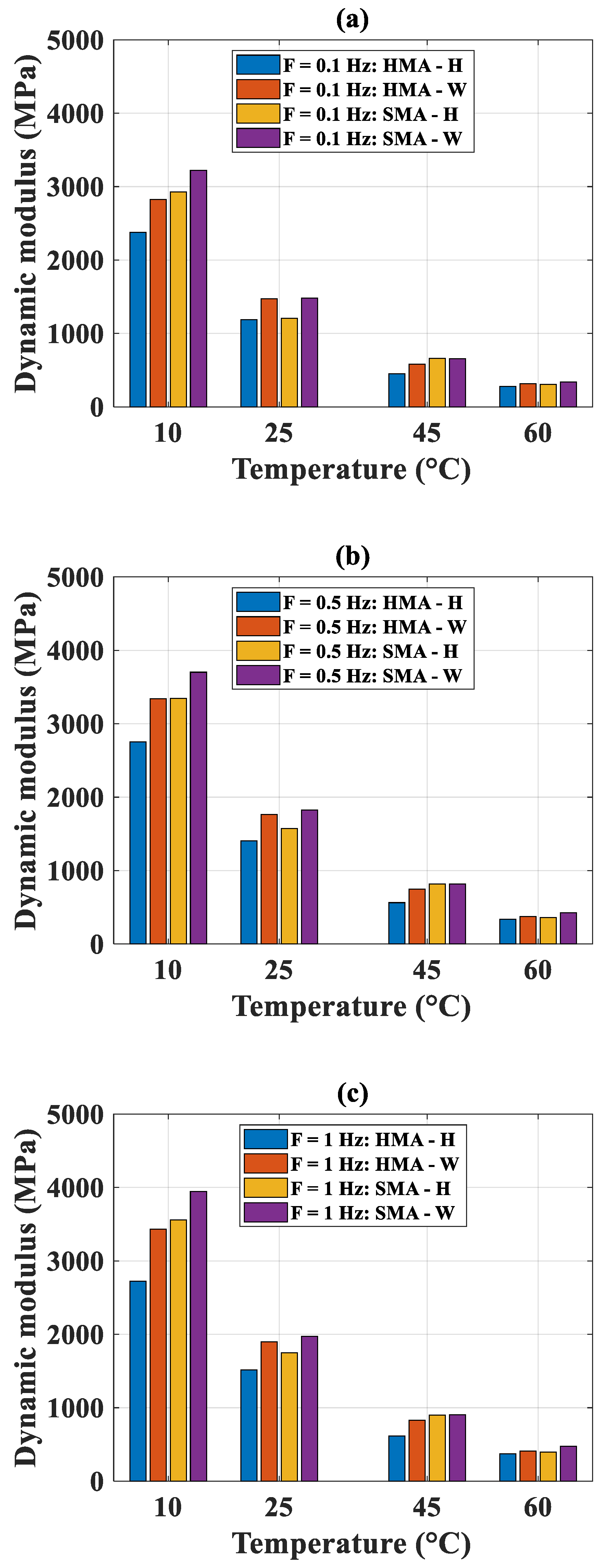
5.1. Experimental Results

Figure 4 shows the experimental results on the dynamic modulus |E*| in highlighting the influence of the testing frequency, whereas Figure 5 shows similar results in highlighting the influence of the testing temperature. Considering a similar testing frequency, an increase of the testing temperature reduced the value of the dynamic modulus |E*|. Besides, at similar testing temperature, an increase of the testing frequency increased the value of the dynamic modulus |E*|. Specifically, the effects of the testing frequency and temperature on the experimental values |E*| are clearly shown in Figure 4 and Figure 5. The highest value of the dynamic modulus |E*| for four types of mixtures was obtained with a temperature of 10 °C and a frequency of 25 Hz. The smallest value of the dynamic modulus |E*| was obtained in the case of 60 °C and 0.1 Hz. At a testing temperature of 10 °C, the value of |E*| of SMA-H was 1.22–1.33 times higher than HMA-H, whereas it was 1.01–1.42 times at 25 °C, 1.45–1.7 times at 45 °C and 1.01–1.08 times at 60 °C. For asphalt mixtures made by hot technology at a similar temperature, the difference was more pronounced with the higher frequency. The difference could be neglected at a testing temperature of 60 °C. At a testing temperature of 10 °C, the value of the dynamic modulus |E*| of SMA-W was 1.11–1.22 times higher than HMA-W, whereas it was 1.01–1.15 times at a temperature of 25 °C, 1.09–1.22 times at a temperature of 45 °C, and 1.08–1.26 times at a temperature of 60 °C.

It could be concluded that, compared to the HMA, the SMA showed superior performance in terms of the dynamic modulus |E*|. Besides, the warm technology exhibited higher dynamic modulus |E*| than using the hot technology. Considering SMA and the mixtures using the warm technique, similar observations were also reported in the literature [12]. Indeed, Al-Qadi et al. showed that the SMA-W exhibited significant improvement compared with SMA-H. Moreover, the authors showed that, in terms of additives, Sasobit disclosed the highest performance compared with the control mix, Evotherm, and foamed asphalt. Besides, the curing time was proved to be another critical factor affecting the dynamic modulus. Several curing times using Sasobit were tested in the work, and the results showed that 1-day curing time was optimal. In this study, taking advantage of such a result, the curing time was directly chosen as one day. The analysis of the effect of curing time might be the objective of further research, as different natures of aggregates, filler, or bitumen might have a certain influence on the dynamic modulus. Besides, another study confirmed the addition of additives enhanced the dynamic modulus compared with the control asphalt mixtures, for instance, in the work of Goh and You [80]. Last but not least, the success in decreasing the mixing and compacting temperatures was proven in the literature but only for recycled aggregates [12,48]; this study showed a similarly successful result of the dynamic modulus of asphalt mixture in using conventional aggregates.

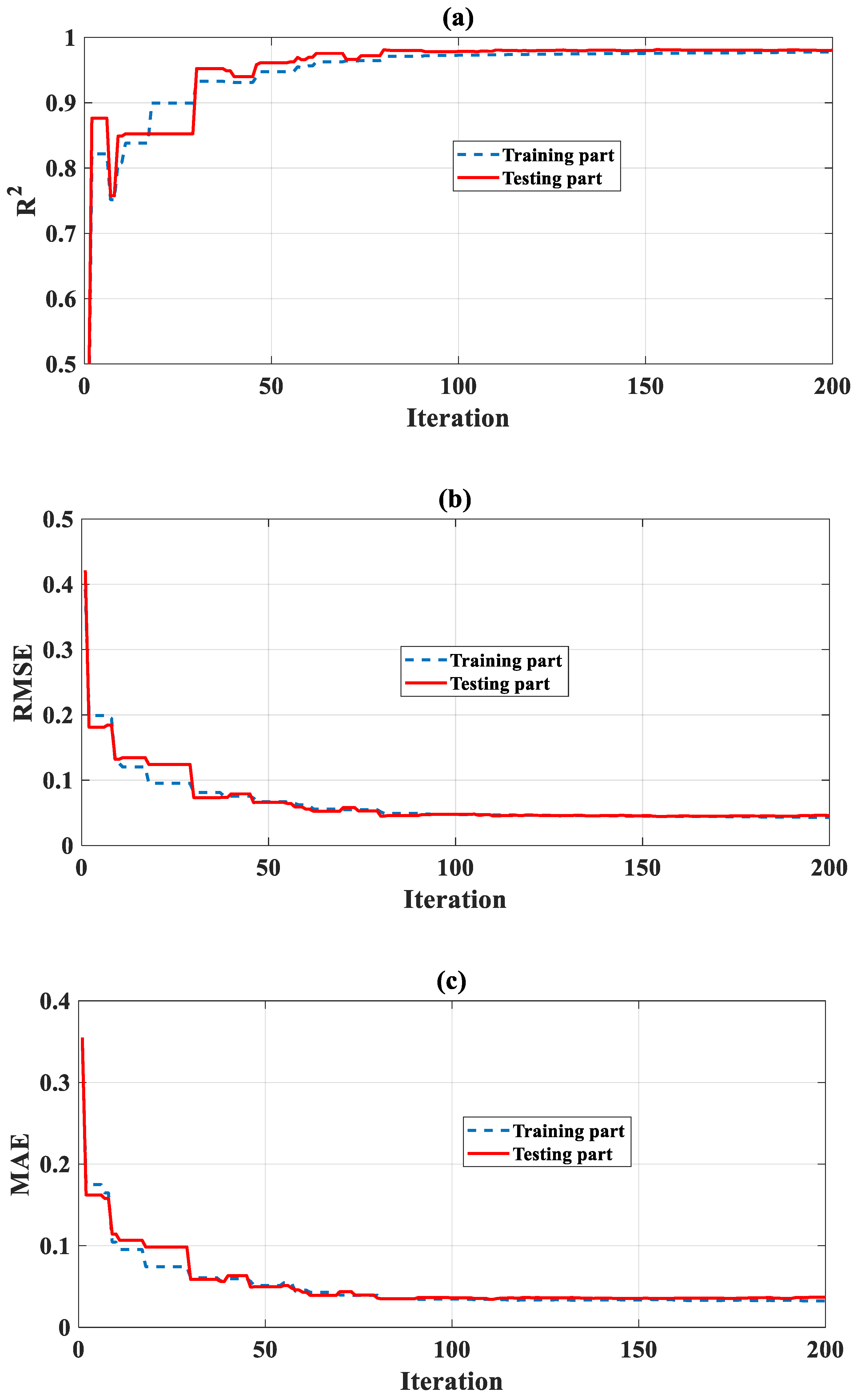
5.2. Optimization of the ANN-TLBO Model

Regarding the development of ANN-TLBO algorithms, the determination of the parameters of such a model is a crucial step. Indeed, the prediction capability is directly dependent on the choice of the appropriate values of parameters. They could be the activation function of the hidden layer, cost function, the training algorithm of the ANN model, or the population size, the stopping criterion of the optimization algorithm. After trial-and-error tests, the parameters of the proposed ANN-TLBO model were chosen and indicated in

Table 5. ANN and TLBO parameters.

Parameter	Value and Description
Number of neurons in output layer	1
Number of weight parameters	31
Number of hidden layers	1
Number of neurons in the input layer	4
Number of neurons in hidden layer	5
Hidden layer activation function	Sigmoid
Output layer activation function	Linear
Cost function	MSE-Mean square error
Training algorithm	TLBO
TLBO population size	30
Stopping iteration	200

. The final structure of ANN-TLBO was 4-5-1 and denoted as ANN-TLBO [4-5-1]. Three statistical measurements (i.e., R², RMSE, and MAE) were applied for ANN-TLBO to find the best values of the weights and biases associated with the neurons. This means that all the results presented herein were the best performance of the proposed ANN-TLBO model, with the highest value of R² and the lowest values of MAE, RMSE concerning one selected dataset. The evaluations of cost functions with respect to R², RMSE, and MAE for predicting the dynamic modulus |E*| are presented in Figure 6. This study focused only on the selection of an appropriate choice of the stopping criterion. Furthermore, the accuracy of the ML algorithm could not be guaranteed by the higher number of iteration, for instance in [81], where the best model was found at 20 over 100 performed iterations. As a result, the convergence of the proposed ANN-TLBO in this study was reached after about 100 iterations, and 200 iterations were sufficient to reach the state of convergence of all the cost functions.

5.3. Validation and Comparison of ANN-TLBO with Single ANN

The performance of the ANN model, in comparison with the ANN-TLBO algorithm, is presented under regression plots (Figure 7), showing a comparison between the predicted and actual values of the dynamic modulus |E*|. The ideal regression lines are in discontinuous style, whereas the R² between predicted and actual dynamic modulus |E*| are given (

Table 6. Summary of prediction capability of the ANN-TLBO model.

Model	Data	RMSE	MAE	ErrorMean	ErrorStD	R2	Slope
Unit		MPa	MPa	MPa	MPa	-	-
ANN	Training	379.035	291.815	−126.527	360.414	0.907	0.914
	Testing	292.828	236.917	−31.099	295.080	0.948	0.932
ANN-TLBO	Training	189.666	153.851	18.639	190.396	0.975	0.958
	Testing	183.308	141.540	21.294	184.511	0.981	0.936
% Gain	Training	+50.0	+47.3	+114.7	+47.2	+7.5	+4.8
	Testing	+37.4	+40.3	+168.5	+37.5	+3.5	+0.4

). The correlation results analysis showed that the R² values were 0.907, 0.948 for the training and testing datasets, respectively, for the ANN model. Concerning the ANN-TLBO model, these values were 0.975, 0.981 for the training and testing datasets, respectively. These results showed a very good prediction performance of the two proposed models. However, using an optimization, the ANN-TLBO was found to be the superior predictor compared with the single ANN.

The summary of the prediction performance of ANN and ANN-TLBO is presented in Table 6. The values of R², RMSE, and MAE were calculated based on the formulations given in the previous section, whereas ErrorMean was the mean values of errors and ErrorStD was the standard deviation of errors. The “Slope” represented the slope between the ideal regression line (discontinuous lines in Figure 7) and the linear fit, given by the models (continuous lines in Figure 7). The two additional error criteria also confirmed that ANN-TLBO is superior to ANN in predicting the dynamic modulus |E*|. For illustration purposes, the values of the dynamic modulus |E*| in function of sample index using individual ANN and ANN-TLBO models are plotted in Figure 8 for the training and testing datasets. It is clearly seen that the predicted values were in excellent agreement with the experimental dynamic modulus |E*| values.

Overall, the prediction capability of ANN-TLBO was quantified based on various performance indicators. The proposed hybrid model showed high prediction capability and outperformed individual ANN, clearly demonstrating the efficiency of using TLBO as an optimization tool.

5.4. Sensitivity Analysis of the Prediction Variables

The sensitivity analysis of the input variables used in the prediction process is presented in this section. The temperature and frequency were successively varied at their range of value, whereas other inputs were kept constant. Precisely, using the ANN-TLBO model developed previously, a new two-dimensional input space was constructed using the value of each input, recorded at ten different quantile levels: 0, 0.1, 0.2, 0.3, 0.4, 0.5, 0.6, 0.7, 0.8, 0.9, and 1.0. The temperature and the frequency were them successively selected, and the model was run eleven times, once for each percentile value. Principally, the method provides quantitative disclosures on the change of output when the selected input changes.

It can be seen that the temperature was the most significant factor influencing the dynamic modulus |E*|, followed by the frequency (Figure 9). While varying two input variables, the sensitivity index varied from [200–300] to [−100] for the temperature, whereas it varied from [0] to [100] for the frequency. Moreover, the nonlinear negative effect was observed for the temperature, whereas a positive linear effect was found for the frequency. These observations were confirmed for all mixtures.

As indicated in many studies [82,83,84,85], exploring the relative importance of inputs might offer better in-depth knowledge of the output, which could directly assist engineers during the preparation phase. Considering the testing temperature and frequency, experimental investigations have been conducted in several works [12,80]. However, a direct linear interpolation of the as-obtained results or missing information on the range of input values could lead to inexact observations. In this work, an attempt was made from an experimental point of view, to cover a broad range of testing temperature and frequency with sufficiently grid points. The dependency of the dynamic modulus on inputs was then analyzed with the developed ML algorithm. For each mixture, a fit equation was proposed to highlight the dependency of the selected variable to dynamic modulus |E*|. With reasonable accuracy, a linear equation was finally adopted to fit the frequency versus the dynamic modulus. On the contrary, a cubic equation was chosen to relate the temperature with the dynamic modulus. Summarized information on the sensitivity analysis of the effect of temperature and frequency is presented in

Table 7. Summary of the sensitivity analysis using the ANN-TLBO algorithm.

Mixture	Technology	Variable	Appropriate Fit	Equation Form	Correlation Effect
HMA	Hot	Frequency	Linear	y = 134.2x − 15	Positive
		Temperature	Cubic	y = −57.09x3 + 428.16x2 − 776.28x + 292.01	Negative
HMA	Warm	Frequency	Linear	y = 94.74x − 11.21	Positive
		Temperature	Cubic	y = 44.97x3 + 158.28x2 − 530.81x + 224.69	Negative
SMA	Hot	Frequency	Linear	y = 96.91x − 11.24	Positive
		Temperature	Cubic	y = 71.46x3 + 135.6x2 − 569.75x + 254.18	Negative
SMA	Warm	Frequency	Linear	y = 112.69x − 17.74	Positive
		Temperature	Cubic	y = 65.66x3 + 102.69x2 − 489.04x + 222.45	Negative

, including the appropriate fit, equation form, and correlation effect. The proposed equations could facilitate the usage of asphalt mixtures in selecting the desired dynamic modulus in function of the testing temperature and frequency.

6. Conclusions and Outlook

In this study, a novel machine learning algorithm, namely ANN-TLBO, was used to predict the dynamic modulus |E*| of SMA, one of the most critical mechanical properties of the asphalt concrete. The proposed model consisted of one well-known machine learning algorithm (ANN) and an effective optimization algorithm (TLBO). The dataset resulting from experiments consisting of 96 entries (average values per 6 of 576 experimental results) was used for the development of the algorithm. The performance of the proposed model was assessed by various common statistical measurements, such as RMSE, MAE, and R.

The validation results showed that the performance of ANN-TLBO was remarkable with ideal values of R² (0.975 for the training part and 0.981 for the testing dataset). Such results were superior to those obtained by a single ANN model (0.907 for the training phase and 0.948 for the testing dataset). In addition, a sensitivity analysis was performed, and the results showed that the testing temperature was the most influential factor in the prediction of the dynamic modulus |E*|. These results indicated that ANN-TLBO could be a promising predictor of the dynamic modulus |E*| of SMA mixtures. It could thus be used in the designing phase of SMA mixtures, aiming at a more effective and efficient process.

Extending the existing database could be a short-term perspective of the present study. This could improve the quality of the dataset and expand the ranges of input variables used in the prediction process. Besides, despite an astonishing performance of ANN-TLBO, the use of alternative machine learning algorithms or optimization techniques should be examined to improve the effectiveness of the prediction algorithm.

References

1. Shen, D.-H.; Kuo, M.-F.; Du, J.-C. Properties of gap-aggregate gradation asphalt mixture and permanent deformation. Constr. Build. Mater. 2005, 19, 147–153. [Google Scholar] [CrossRef]
2. Murali Krishnan, J.; Rajagopal, K.R. Review of the uses and modeling of bitumen from ancient to modern times. Appl. Mech. Rev. 2003, 56, 149–214. [Google Scholar] [CrossRef]
3. Capitão, S.D.; Picado-Santos, L.G.; Martinho, F. Pavement engineering materials: Review on the use of warm-mix asphalt. Constr. Build. Mater. 2012, 36, 1016–1024. [Google Scholar] [CrossRef]
4. Jamshidi, A.; Hamzah, M.O.; You, Z. Performance of warm mix asphalt containing sasobit®: State-of-the-Art. Constr. Build. Mater. 2013, 38, 530–553. [Google Scholar] [CrossRef]
5. Sangiorgi, C.; Tataranni, P.; Simone, A.; Vignali, V.; Lantieri, C.; Dondi, G. Stone mastic asphalt (SMA) with crumb rubber according to a new dry-hybrid technology: A laboratory and trial field evaluation. Constr. Build. Mater. 2018, 182, 200–209. [Google Scholar] [CrossRef]
6. Wang, H.; Liu, X.; Apostolidis, P.; Scarpas, T. Review of warm mix rubberized asphalt concrete: Towards a sustainable paving technology. J. Clean. Prod. 2018, 177, 302–314. [Google Scholar] [CrossRef] [Green Version]
7. Witczak, M.W.; Fonseca, O.A. Revised predictive model for dynamic (complex) modulus of asphalt mixtures. Transp. Res. Rec. 1996, 1540, 15–23. [Google Scholar] [CrossRef]
8. Silva, H.M.R.D.; Oliveira, J.; Ferreira, C.I.G.; Pereira, P.A.A. Assessment of the performance of warm mix asphalts in road pavements. Int. J. Pavement Res. Technol. 2010, 3, 119–127. [Google Scholar]
9. Sanchez-Alonso, E.; Vega-Zamanillo, A.; Castro-Fresno, D.; DelRio-Prat, M. Evaluation of compactability and mechanical properties of bituminous mixes with warm additives. Constr. Build. Mater. 2011, 25, 2304–2311. [Google Scholar] [CrossRef]
10. Zaumanis, M. Warm Mix Asphalt Investigation. Master’s Thesis, Technical University of Denmark in cooperation with the Danish Road Institute, Kgs. Lyngby, Denmark, 2010. [Google Scholar]
11. Peinado, D.; de Vega, M.; García-Hernando, N.; Marugán-Cruz, C. Energy and exergy analysis in an asphalt plant’s rotary dryer. Appl. Therm. Eng. 2011, 31, 1039–1049. [Google Scholar] [CrossRef] [Green Version]
12. Al-Qadi, I.L.; Baek, J.; Leng, Z.; Wang, H.; Doyen, M.; Kern, J.; Gillen, S. Short-Term Performance of Modified Stone Matrix Asphalt (SMA) Produced with Warm Mix Additives; Technical Report; Illinois Center for Transportation: Rantoul, IL, USA, 2012. [Google Scholar]
13. Zaumanis, M.; Mallick, R.B.; Frank, R. 100% recycled hot mix asphalt: A review and analysis. Resour. Conserv. Recycl. 2014, 92, 230–245. [Google Scholar] [CrossRef]
14. Petersen, J.C. A review of the fundamentals of asphalt oxidation: Chemical, physicochemical, physical property, and durability relationships. Transp. Res. Circ. 2009. [Google Scholar] [CrossRef]
15. Baghaee Moghaddam, T.; Baaj, H. The use of rejuvenating agents in production of recycled hot mix asphalt: A systematic review. Constr. Build. Mater. 2016, 114, 805–816. [Google Scholar] [CrossRef]
16. D’Angelo, J.; Cowsert, J.; Newcomb, D.D. Warm-Mix Asphalt: European Practice; No. FHWA-PL-08-007; United States, Federal Highway Administration, Office of International Programs: Washington, DC, USA, 2008. [Google Scholar]
17. Rubio, M.C.; Martínez, G.; Baena, L.; Moreno, F. Warm mix asphalt: An overview. J. Clean. Prod. 2012, 24, 76–84. [Google Scholar] [CrossRef]
18. Prowell, B.D.; Hurley, G.C.; Crews, E. Field performance of warm-mix asphalt at national center for asphalt technology test track. Transp. Res. Rec. 2007, 1998, 96–102. [Google Scholar] [CrossRef]
19. Graham, C.H.; Brian, D.P. Evaluation of Aspha-Min® Zeolite for Use in Warm Mix Asphalt; NCAT Report 05-04; Auburn University: Auburn, AL, USA, 2005. [Google Scholar]
20. Olard, F.; Noanc, L.E. Low energy asphalts. In Proceedings of the 23rd Piarc World Road Congress, Paris, France, 17–21 September 2007. [Google Scholar]
21. Jullien, A.; Baudru, Y.; Tamagny, P.; Olard, F.; Zavan, D. A Comparison of Environmental Impacts of Hot and Warm Mix Asphalt; World Road Association—PIARC: Paris, France, 2011. [Google Scholar]
22. Bari, J. Development of a New Revised Version of the Witczak E* Predictive Models for Hot Mix Asphalt Mixtures; Arizona State University: Tempe, AZ, USA, 2005. [Google Scholar]
23. Flintsch, G.W.; Loulizi, A.; Diefenderfer, S.D.; Diefenderfer, B.K.; Galal, K.A. Asphalt material characterization in support of mechanistic–empirical pavement design guide implementation in virginia. Transp. Res. Rec. 2008, 2057, 114–125. [Google Scholar] [CrossRef]
24. Birgisson, B.; Sholar, G.; Roque, R. Evaluation of a predicted dynamic modulus for florida mixtures. Transp. Res. Rec. 2005, 1929, 200–207. [Google Scholar] [CrossRef]
25. Sakhaeifar, M.S.; Richard Kim, Y.; Kabir, P. New predictive models for the dynamic modulus of hot mix asphalt. Constr. Build. Mater. 2015, 76, 221–231. [Google Scholar] [CrossRef]
26. Shu, X.; Huang, B. Micromechanics-Based dynamic modulus prediction of polymeric asphalt concrete mixtures. Compos. Part B Eng. 2008, 39, 704–713. [Google Scholar] [CrossRef]
27. Shu, X.; Huang, B. Predicting dynamic modulus of asphalt mixtures with differential method. Road Mater. Pavement Des. 2009, 10, 337–359. [Google Scholar] [CrossRef]
28. Cho, Y.-H.; Park, D.-W.; Hwang, S.-D. A predictive equation for dynamic modulus of asphalt mixtures used in Korea. Constr. Build. Mater. 2010, 24, 513–519. [Google Scholar] [CrossRef]
29. Rahman, A.A.; Islam, M.R.; Tarefder, R.A. Dynamic modulus and phase angle models for New Mexico’s superpave mixtures. Road Mater. Pavement Des. 2019, 20, 740–753. [Google Scholar] [CrossRef]
30. Ceylan, H.; Gopalakrishnan, K.; Kim, S. Looking to the future: The next-generation hot mix asphalt dynamic modulus prediction models. Int. J. Pavement Eng. 2009, 10, 341–352. [Google Scholar] [CrossRef]
31. Far, M.S.S.; Underwood, B.S.; Ranjithan, S.R.; Kim, Y.R.; Jackson, N. Application of Artificial neural networks for estimating dynamic modulus of asphalt concrete. Transp. Res. Rec. 2009, 2127, 173–186. [Google Scholar] [CrossRef]
32. Sakhaeifar, M.S.; Underwood, B.S.; Kim, Y.R.; Puccinelli, J.; Jackson, N. Development of artificial neural network predictive models for populating dynamic moduli of long-term pavement performance sections. Transp. Res. Rec. 2010, 2181, 88–97. [Google Scholar] [CrossRef]
33. Dharamveer, S.; Musharraf, Z. Commuri sesh artificial neural network modeling for dynamic modulus of hot mix asphalt using aggregate shape properties. J. Mater. Civ. Eng. 2013, 25, 54–62. [Google Scholar] [CrossRef]
34. Olidis, C.; Hein, D. Guide for the mechanistic-empirical design of new and rehabilitated pavement structures materials characterization: Is your agency ready. In Proceedings of the 2004 Annual Conference of the Transportation Association of Canada, Quebec City, QC, Canada, 19–22 September 2004. [Google Scholar]
35. Andrei, D.; Witczak, M.W.; Mirza, M.W. Development of a revised predictive model for the dynamic (complex) modulus of asphalt mixtures. In Development of the 2002 Guide for the Design of New and Rehabilitated Pavement Structures; NCHRP: Washington, DC, USA, 1999. [Google Scholar]
36. Christensen, D.W., Jr.; Pellinen, T.; Bonaquist, R.F. Hirsch model for estimating the modulus of asphalt concrete. J. Assoc. Asph. Paving Technol. 2003, 72, 97–121. [Google Scholar]
37. Al-Khateeb, G.; Shenoy, A.; Gibson, N.; Harman, T. A new simplistic model for dynamic modulus predictions of asphalt paving mixtures. J. Assoc. Asph. Paving Technol. 2006, 75, 1–40. [Google Scholar]
38. Obulareddy, S. Fundamental characterization of Louisiana HMA mixtures for the 2002 mechanistic-empirical design guide. LSU Master’s Theses, Andhra University, Visakhapatnam, India, 2006. [Google Scholar]
39. Dongre, R.; Myers, L.; D’Angelo, J.; Paugh, C.; Gudimettla, J. Field evaluation of Witczak and Hirsch models for predicting dynamic modulus of hot-mix asphalt (with discussion). J. Assoc. Asph. Paving Technol. 2005, 74, 381–442. [Google Scholar]
40. Tran, N.; Hall, K. Evaluating the predictive equation in determining dynamic moduli of typical asphalt mixtures used in Arkansas. Natl. Acad. Sci. Eng. Med. 2005, 74E, 1–17. [Google Scholar]
41. Azari, H.; Al-Khateeb, G.; Shenoy, A.; Gibson, N. Comparison of simple performance test |E*| of accelerated loading facility mixtures and prediction |E*| use of NCHRP 1-37A and witczak’s new equations. Transp. Res. Rec. 2007, 1998, 1–9. [Google Scholar] [CrossRef]
42. Kim, Y.R.; King, M.; Momen, M. Typical dynamic moduli values of hot mix asphalt in North Carolina and their prediction. In Proceedings of the Transportation Research Board 84th Annual Meeting compendium of papers CD-ROM, Washington, DC, USA, 9–13 January 2005; pp. 5–2568. [Google Scholar]
43. Schwartz, C.W. Evaluation of the Witczak dynamic modulus prediction model. In Proceedings of the 84th Annual Meeting of the Transportation Research Board, Washington, DC, USA, 9–13 January 2005. [Google Scholar]
44. Pellinen, T.K.; Witczak, M.W. Use of stiffness of hot-mix asphalt as a simple performance test. Transp. Res. Rec. 2002, 1789, 80–90. [Google Scholar] [CrossRef]
45. ARA, I. Guide for Mechanistic–Empirical Design of New and Rehabilitated Pavement Structures; Final Report, NCHRP Project 1-37A; ERES Division 505 West University Avenue Champaign: Champaign, IL, USA, 2004. [Google Scholar]
46. Abdo, A.A.; Bayomy, F.; Nielsen, R.; Weaver, T.; Jung, S.J.; Santi, M.J. Prediction of the dynamic modulus of Superpave mixes. In Proceedings of the 8th International Conference on the Bearing Capacity of Roads, Railways and Airfields (BCR2A’09), Champaign, IL, USA, 29 June–2 July 2009; pp. 305–314. [Google Scholar]
47. Ceylan, H.; Gopalakrishnan, K.; Kim, S. Advanced approaches to hot-mix asphalt dynamic modulus prediction. Can. J. Civ. Eng. 2008, 35, 699–707. [Google Scholar] [CrossRef]
48. Al-Qadi, I.L.; Leng, Z.; Baek, J.; Wang, H.; Doyen, M.; Gillen, S.L. Short-Term performance of plant-mixed warm stone mastic asphalt: Laboratory testing and field evaluation. Transp. Res. Rec. 2012, 2306, 86–94. [Google Scholar] [CrossRef]
49. Leng, Z.; Gamez, A.; Al-Qadi, I.L. Mechanical property characterization of warm-mix asphalt prepared with chemical additives. J. Mater. Civ. Eng. 2014, 26, 304–311. [Google Scholar] [CrossRef]
50. AASHTO M 325-08. Available online: https://www.techstreet.com/standards/aashto-m-325-08-2017?product_id=1583186 (accessed on 18 March 2020).
51. Vietnam Standard, M. of T. of V. Vietnam Standard—Guiding the Application of the Current System of Technical Standards to Enhance the Quality Management of the Design and Construction of Hot Mix Asphalt for Large-Scale Roads, Issued; Tổng cục Tiêu chuẩn Đo lường Chất lượng: Hanoi, Vietnam, 2014. [Google Scholar]
52. AASHTO TP 62—Standard Method of Test for Determining Dynamic Modulus of Hot Mix Asphalt (HMA) | Engineering360. Available online: https://standards.globalspec.com/std/1283471/AASHTO%20TP%2062 (accessed on 27 December 2019).
53. Pham, B.T.; Nguyen, M.D.; Bui, K.-T.T.; Prakash, I.; Chapi, K.; Bui, D.T. A novel artificial intelligence approach based on multi-layer perceptron neural network and biogeography-based optimization for predicting coefficient of consolidation of soil. Catena 2019, 173, 302–311. [Google Scholar] [CrossRef]
54. Dao, D.V.; Ly, H.-B.; Trinh, S.H.; Le, T.-T.; Pham, B.T. Artificial intelligence approaches for prediction of compressive strength of geopolymer concrete. Materials 2019, 12, 983. [Google Scholar] [CrossRef] [Green Version]
55. Bayat, M.; Ghorbanpour, M.; Zare, R.; Jaafari, A.; Pham, B.T. Application of artificial neural networks for predicting tree survival and mortality in the Hyrcanian forest of Iran. Comput. Electron. Agric. 2019, 164, 104929. [Google Scholar] [CrossRef]
56. Shahin, M.A.; Jaksa, M.B.; Maier, H.R. Artificial neural network applications in geotechnical engineering. Aust. Geomech. 2001, 36, 49–62. [Google Scholar]
57. Zhang, Z.; Friedrich, K. Artificial neural networks applied to polymer composites: A review. Compos. Sci. Technol. 2003, 63, 2029–2044. [Google Scholar] [CrossRef]
58. Sha, W.; Edwards, K. The use of artificial neural networks in materials science based research. Mater. Des. 2007, 28, 1747–1752. [Google Scholar] [CrossRef]
59. Črepinšek, M.; Liu, S.-H.; Mernik, L. A note on teaching–learning-based optimization algorithm. Inf. Sci. 2012, 212, 79–93. [Google Scholar] [CrossRef]
60. Rao, R.V.; Savsani, V.J.; Vakharia, D. Teaching-Learning-Based optimization: A novel method for constrained mechanical design optimization problems. Comput. Aided Des. 2011, 43, 303–315. [Google Scholar] [CrossRef]
61. Zou, F.; Wang, L.; Hei, X.; Chen, D. Teaching-Learning-Based optimization with learning experience of other learners and its application. Appl. Soft Comput. 2015, 37, 725–736. [Google Scholar] [CrossRef]
62. Rao, R.V.; Savsani, V.J.; Vakharia, D. Teaching-Learning-Based optimization: An optimization method for continuous non-linear large scale problems. Inf. Sci. 2012, 183, 1–15. [Google Scholar] [CrossRef]
63. Khorsheed, M.S.; Al-Thubaity, A.O. Comparative evaluation of text classification techniques using a large diverse Arabic dataset. Lang Resour. Eval. 2013, 47, 513–538. [Google Scholar] [CrossRef]
64. Leema, N.; Nehemiah, H.K.; Kannan, A. Neural network classifier optimization using differential evolution with global information and back propagation algorithm for clinical datasets. Appl. Soft Comput. 2016, 49, 834–844. [Google Scholar] [CrossRef]
65. Pham, B.T.; Nguyen, M.D.; Van Dao, D.; Prakash, I.; Ly, H.-B.; Le, T.-T.; Ho, L.S.; Nguyen, K.T.; Ngo, T.Q.; Hoang, V. Development of artificial intelligence models for the prediction of compression coefficient of soil: An application of Monte Carlo sensitivity analysis. Sci. Total Environ. 2019, 679, 172–184. [Google Scholar] [CrossRef]
66. Asteris, P.G.; Mokos, V.G. Concrete compressive strength using artificial neural networks. Neural Comput. Appl. 2019. [Google Scholar] [CrossRef]
67. Asteris, P.G.; Ashrafian, A.; Rezaie-Balf, M. Prediction of the compressive strength of self-compacting concrete using surrogate models. Comput. Concr. 2019, 24, 137–150. [Google Scholar]
68. Asteris, P.G.; Kolovos, K.G. Self-compacting concrete strength prediction using surrogate models. Neural Comput. Appl. 2019, 31, 409–424. [Google Scholar] [CrossRef]
69. Asteris, P.G.; Armaghani, D.J.; Hatzigeorgiou, G.D.; Karayannis, C.G.; Pilakoutas, K. Predicting the shear strength of reinforced concrete beams using artificial neural networks. Comput. Concr. 2019, 24, 469–488. [Google Scholar]
70. Asteris, P.G.; Apostolopoulou, M.; Skentou, A.D.; Moropoulou, A. Application of artificial neural networks for the prediction of the compressive strength of cement-based mortars. Comput. Concr. 2019, 24, 329–345. [Google Scholar]
71. Duan, J.; Asteris, P.G.; Nguyen, H.; Bui, X.-N.; Moayedi, H. A novel artificial intelligence technique to predict compressive strength of recycled aggregate concrete using ICA-XGBoost model. Eng. Comput. 2020, 1–18. [Google Scholar] [CrossRef]
72. Asteris, P.G.; Plevris, V. Anisotropic masonry failure criterion using artificial neural networks. Neural Comput. Appl. 2017, 28, 2207–2229. [Google Scholar] [CrossRef]
73. Asteris, P.G.; Nikoo, M. Artificial bee colony-based neural network for the prediction of the fundamental period of infilled frame structures. Neural Comput. Appl. 2019, 31, 4837–4847. [Google Scholar] [CrossRef]
74. Ly, H.-B.; Monteiro, E.; Le, T.-T.; Le, V.M.; Dal, M.; Régnier, G.; Pham, B.T. Prediction and sensitivity analysis of bubble dissolution time in 3D selective laser sintering using ensemble decision trees. Materials 2019, 12, 1544. [Google Scholar] [CrossRef] [Green Version]
75. Nguyen, H.-L.; Le, T.-H.; Pham, C.-T.; Le, T.-T.; Ho, L.S.; Le, V.M.; Pham, B.T.; Ly, H.-B. Development of hybrid artificial intelligence approaches and a support vector machine algorithm for predicting the Marshall parameters of stone matrix asphalt. Appl. Sci. 2019, 9, 3172. [Google Scholar] [CrossRef] [Green Version]
76. Nguyen, H.-L.; Pham, B.T.; Son, L.H.; Thang, N.T.; Ly, H.-B.; Le, T.-T.; Ho, L.S.; Le, T.-H.; Tien Bui, D. Adaptive network based fuzzy inference system with meta-heuristic optimizations for international roughness index prediction. Appl. Sci. 2019, 9, 4715. [Google Scholar] [CrossRef] [Green Version]
77. Pham, B.T.; Le, L.M.; Le, T.-T.; Bui, K.-T.T.; Le, V.M.; Ly, H.-B.; Prakash, I. Development of advanced artificial intelligence models for daily rainfall prediction. Atmos. Res. 2020, 237, 104845. [Google Scholar] [CrossRef]
78. Phong, T.V.; Phan, T.T.; Prakash, I.; Singh, S.K.; Shirzadi, A.; Chapi, K.; Ly, H.-B.; Ho, L.S.; Quoc, N.K.; Pham, B.T. Landslide susceptibility modeling using different artificial intelligence methods: A case study at Muong Lay district, Vietnam. Geocarto Int. 2019, 1–24. [Google Scholar] [CrossRef]
79. Le, T.-T.; Pham, B.T.; Ly, H.-B.; Shirzadi, A.; Le, L.M. Development of 48-hour precipitation forecasting model using nonlinear autoregressive neural network. In Proceedings of the CIGOS 2019, Innovation for Sustainable Infrastructure; Ha-Minh, C., Dao, D.V., Benboudjema, F., Derrible, S., Huynh, D.V.K., Tang, A.M., Eds.; Springer: Singapore, 2020; pp. 1191–1196. [Google Scholar]
80. Goh, S.W.; You, Z. Resilient modulus and dynamic modulus of warm mix asphalt. In Proceedings of the GeoCongress 2008: Geosustainability and Geohazard Mitigation, New Orleans, LA, USA, 9–12 March 2008; pp. 1000–1007. [Google Scholar]
81. Ly, H.-B.; Le, L.M.; Duong, H.T.; Nguyen, T.C.; Pham, T.A.; Le, T.-T.; Le, V.M.; Nguyen-Ngoc, L.; Pham, B.T. Hybrid Artificial intelligence approaches for predicting critical buckling load of structural members under compression considering the influence of initial geometric imperfections. Appl. Sci. 2019, 9, 2258. [Google Scholar] [CrossRef] [Green Version]
82. Qi, C.; Tang, X.; Dong, X.; Chen, Q.; Fourie, A.; Liu, E. Towards Intelligent mining for backfill: A genetic programming-based method for strength forecasting of cemented paste backfill. Miner. Eng. 2019, 133, 69–79. [Google Scholar] [CrossRef]
83. Dao, D.V.; Adeli, H.; Ly, H.-B.; Le, L.M.; Le, V.M.; Le, T.-T.; Pham, B.T. A Sensitivity and robustness analysis of GPR and ANN for high-performance concrete compressive strength prediction using a monte carlo simulation. Sustainability 2020, 12, 830. [Google Scholar] [CrossRef] [Green Version]
84. Ly, H.-B.; Le, T.-T.; Le, L.M.; Tran, V.Q.; Le, V.M.; Vu, H.-L.T.; Nguyen, Q.H.; Pham, B.T. Development of Hybrid machine learning models for predicting the critical buckling load of I-shaped cellular beams. Appl. Sci. 2019, 9, 5458. [Google Scholar] [CrossRef] [Green Version]
85. Dao, D.V.; Ly, H.-B.; Vu, H.-L.T.; Le, T.-T.; Pham, B.T. Investigation and optimization of the C-ANN structure in predicting the compressive strength of foamed concrete. Materials 2020, 13, 1072. [Google Scholar] [CrossRef] [Green Version]
Figure 1. Mixture gradation aggregate (a) Stone Mastic Asphalt (SMA) samples, (b) hot mix asphalt (HMA) samples.
Applsci 10 05242 g001
Figure 2. The SMA samples preparation and testing: (a) Asphalt mixer, (b) The SMA and HMA samples.
Applsci 10 05242 g002
Figure 3. The SMA samples preparation and testing: (a) Gyratory Compactor machine, (b) CRT NU-14 machine.
Applsci 10 05242 g003
Figure 4. Experimental results of dynamic modulus |E*| in function of the frequency, in the case of (a) SMA-W; (b) SMA-H; (c) HMA-W; and (d) HMA-H.
Applsci 10 05242 g004aApplsci 10 05242 g004b
Figure 5. Experimental results of dynamic modulus |E*| in function of the test temperature for different frequencies: (a) 0.1 Hz; (b) 0.5 Hz; (c) 1 Hz; (d) 5 Hz; (e) 10 Hz; (f) 25 Hz.
Applsci 10 05242 g005aApplsci 10 05242 g005b
Figure 6. Optimization of weight parameters of ANN models using the TLBO algorithm: (a) R2, (b) RMSE, and (c) MAE.
Applsci 10 05242 g006
Figure 7. Regression graphs using individual ANN model: (a) training and (b) testing parts; ANN-TLBO model: (c) training and (d) testing parts.
Applsci 10 05242 g007
Figure 8. Dynamic modulus in function of sample index, using individual ANN model for (a) training part and (b) testing part, using ANN-TLBO model for (c) training part and (d) testing part.
Applsci 10 05242 g008aApplsci 10 05242 g008b
Figure 9. Sensitivity index of frequency and temperature for four combinations of SMA, HMA, H, and W.
Applsci 10 05242 g009