Pansharpening by Complementing Compressed Sensing with Spectral Correction


Graduate School of Engineering, Tohoku University, Sendai, Miyagi 980-8579, Japan
*
Author to whom correspondence should be addressed.
Appl. Sci. 2020, 10(17), 5789; https://0-doi-org.brum.beds.ac.uk/10.3390/app10175789
Submission received: 30 June 2020
/
Revised: 8 August 2020
/
Accepted: 18 August 2020
/
Published: 21 August 2020
(This article belongs to the Special Issue Advances in Image Processing, Analysis and Recognition Technology)
Abstract
:Featured Application
Satellite image processing for change detection, target recognition, classification, map application, visual image analysis, etc.
Abstract
Pansharpening (PS) is a process used to generate high-resolution multispectral (MS) images from high-spatial-resolution panchromatic (PAN) and high-spectral-resolution multispectral images. In this paper, we propose a method for pansharpening by focusing on a compressed sensing (CS) technique. The spectral reproducibility of the CS technique is high due to its image reproducibility, but the reproduced image is blurry. Although methods of complementing this incomplete reproduction have been proposed, it is known that the existing method may cause ringing artifacts. On the other hand, component substitution is another technique used for pansharpening. It is expected that the spatial resolution of the images generated by this technique will be as high as that of the high-resolution PAN image, because the technique uses the corrected intensity calculated from the PAN image. Based on these facts, the proposed method fuses the intensity obtained by the component substitution method and the intensity obtained by the CS technique to move the spatial resolution of the reproduced image close to that of the PAN image while reducing the spectral distortion. Experimental results showed that the proposed method can reduce spectral distortion and maintain spatial resolution better than the existing methods.
1. Introduction
The optical sensors installed in satellites acquire panchromatic (PAN) and multispectral (MS) region images. PAN sensors observe a wide range of visible and near-infrared (NIR) regions as one band with a high spatial resolution, and the MS sensor observes multiple bands. Pansharpening (PS) is a method used to generate a high-resolution MS images from these two types of data. Due to physical constraints [1], MS sensors are not designed to acquire high-resolution images. In general, high-resolution MS images are obtained via the pansharpening process. PS techniques are used for change detection, target recognition, classification, backgrounds for map application, visual image analysis, etc.
PS has been studied for decades [2,3], and its methodologies can roughly be classified into four types. The first is methods used to generate a pansharpened image by substituting the intensity component of the MS images for that of the PAN image via component substitution. The intensity–hue–saturation (IHS) transform [4], generalized IHS method (GIHS) [5], Brovey transform [6], principal component analysis [6], and Gram–Schmidt transform [7] belong to this group. The second group contains methods used to extract high-frequency components of PAN images via multiresolution analysis (MRA) and then add them to the MS images. To extract high-frequency components, high-pass filter, decimated wavelet transforms [8], a “trous” wavelet transform [9], Laplacian pyramid [10,11], and non-subsampled contourlet transform [12] methods are used. The third group contains methods that use machine-learning techniques such as compressed sensing [13] and deep learning [14,15]. The fourth group is the hybrid methods that combine multiple methods described above. The methods proposed by Vivone et al. [16], Fei et al. [17], and Yin [18] are the ones that combined the component substitution method and the MRA. The combination of the MRA, convolutional neural network (CNN), and sparse modeling was proposed by Wang et al. [19], and the combination of the MRA and CNN was proposed by He et al. [20].
Recently, proposals for hybrid methods using machine-learning techniques have been increasing. Many methods based on compressed sensing (CS) have been proposed based on the 2006 theory [21]. Since Yang et al. [13] proposed a method for super-resolution, it has been frequently applied to PS. Li et al. proposed a method using a learning-free dictionary and CS [22], followed by the proposal of a method using dictionary learning and CS [23]. Although they showed the possibility of using a dictionary without learning, the feasibility of these methods was low because high-resolution MS images that were not realistically available were necessary for dictionary construction. Jiang et al. proposed a method using a high-resolution dictionary generated using a set of pairs of low-resolution MS images and high-resolution PAN images [24]. They then proposed a method for reconstruction by calculating sparse representations in two stages using a learning-free dictionary [25]. Zhu et al. constructed a pair of high-resolution and low-resolution learning-free dictionaries from PAN images [26,27]. Guo et al. proposed a method called online coupled dictionary learning (OCDL) [28], which iteratively performs dictionary learning and reconstruction processes until the reconstructed image becomes stable, based on the sparse representation (SR) theory described by Elad [29]. SR theory shows that better reconstruction results are obtained when the dictionary’s atoms are highly related to the reconstructed image. Vicinanze et al. proposed the generation of a learning-free dictionary using the high-resolution and low-resolution dictionaries as the detailed image information [30]. Ghahremani et al. proposed a learning-free dictionary with low-resolution PAN images and high-resolution detailed information extracted from by the ripplet transform of the edges and textures of high-resolution PAN images [31]. Zhang et al. introduced non-negative matrix factorization and proposed estimation of a high-resolution matrix by solving an optimization problem of decomposing the matrix into basis and coefficient matrices [32]. Ayas et al. created a dictionary of high-resolution MS image features by incorporating the tradeoff parameter [24,26] and back-projection [13,33]. It was shown that the spectral distortion was reduced by incorporating back-projection. Yin proposed the cross-resolution projection and the offset [18]. The cross-resolution projection generates high-resolution MS images by assuming that the position estimated by CS is the same for high-resolution and low-resolution images. The offset is used to adjust the reconstructed image.
In these studies, the results of PS depended on the model selection and dictionary selection. Various studies on the structure and construction of dictionaries, model construction, and optimization processes have been conducted. In addition, it was pointed out that CS-based reconstruction does not guarantee the reproduction of the original image [13,29,34], which means that the spatial characteristics may not be incorporated accurately. The fact that it is not an exact reconstruction should be considered when the method is used for spectral analysis. The process of back-projection was introduced by Yang et al. [13] to improve the reconstructed image. This process was also incorporated by Ayas et al. [34] to reduce the spectral distortion. On the other hand, it is also known that ringing artefacts occur when back-projection is performed. In the PS process, low spectral distortion is important as well as high resolution. It is important to consider how to achieve the fidelity of the reproduced image to the ideal image in terms of the spectral and spatial resolution.
In this paper, we focused on reducing the spectral distortion more effectively than the back-projection for resolution enhancement of a visible light image. To this end, we propose a method for pansharpening by combining the CS technique and a component substitution method that calculates the intensity with high spatial resolution and low spectral distortion to enhance the reproducibility. As the component substitution, spectrum correction using modeled panchromatic image (SCMP) [35] is introduced. The observation band of the PAN sensor of IKONOS, an earth observation satellite, was 526–929 nm. The red, green, blue, and NIR bands of the MS sensor of IKONOS were 632–698 nm, 505–595 nm, 445–516 nm, and 757–853 nm, respectively. Therefore, the PAN sensor covered the observation band of the MS sensor including NIR. The NIR information needs to be included when generating PS images using component substitution in order to avoid spectral distortion. The SCMP is a model that can correct this distortion. On the other hand, processing using the CS is expected to have high data reproducibility and it reflects the characteristics of the input image, while the resolution is lower than that generated by the SCMP. In order to improve the fidelity of the reproduced image to the original image, a tradeoff process was applied on the high-resolution intensity images obtained by the CS and the SCMP. It was found that a spatial resolution equivalent to that of PAN image was obtained and spectral distortion was reduced by the proposed method.
2. Materials and Methods
2.1. Image Datasets
Table 1 shows the two image datasets used for the experiments. The first was collected in May 2008 and covers the city of Nihonmatsu, Japan. The second was collected in May 2006 and covers the city of Yokohama, Japan. The two IKONOS images datasets were provided by the Japan Space Imaging Corporation, Japan. The spatial resolutions of the PAN and the MS images in these datasets were 1 m and 4 m, respectively. The original dataset contained PAN images with 1024 × 1024 pixels and MS images with 256 × 256 pixels for Nihonmatsu, and PAN images with 1792 × 1792 pixels and MS images with 448 × 448 pixels for Yokohama.
The training image datasets had high-resolution PAN images with 256 × 256 pixels for Nihonmatsu, and high-resolution PAN images with 448 × 448 pixels for the Yokohama.
To evaluate the quality of the PS images, we experimented with the test images and original images according to the Wald protocol [36]. The test images were used to evaluate the numerical image quality, and the original images were used as reference images for numerical and visual evaluation. We regarded the original images as ground truth images. The spatial resolution of the test PAN images was reduced from 1 to 4 m and that of the test MS images was reduced from 4 to 16 m. Hence, the test image datasets had PAN images with 256 × 256 pixels and MS images with 64 × 64 pixels for the Nihonmatsu, and PAN images with 448 × 448 pixels and MS images with 112 × 112 pixels for the Yokohama. The training and test images were downsampled images of the original image with bicubic spline interpolation.
2.2. Compressed Sensing
Compressed sensing (CS) is a technique used to reconstruct unknown data from a small number of observed data. In theory, the original data can be estimated when the data is sparse [28]. We considered the problem of reconstructing an image with a higher resolution than the observed low-resolution image . The relationship between the high-resolution image and the low-resolution image can be expressed by Equation (1).
where is a downsampling operator and is a filter that lowers the resolution. At this time, since the dimensionality of is smaller than that of , the solution cannot be uniquely determined.
Based on the compressed sensing theory, the high-resolution image is estimated by Equation (2) from the image element and sparse representation . The element for reproducing the image is called atom , and the set of atoms is called the dictionary .
Using Equation (2), Equation (1) can be expressed as
can be reproduced by using the sparse representation obtained from Equation (4), in which the sparsity constraint is added to Equation (3).
Equation (4) can be solved using optimization methods.
2.3. Proposed Method
Our proposed method combines the advantages of super-resolution based on the theory of compressed sensing and component substitution. In this method, the high-resolution intensity obtained by the SCMP and the high-resolution intensity obtained by the CS-based method are linearly combined using the tradeoff process, and the obtained high-resolution intensity images are fused via the GIHS method to generate PS images. The flow of the proposed method is shown in Figure 1.
2.4. Notation
In the proposed method, four features are extracted from low-resolution images, and the set of features is called the feature map. We used the gradient map proposed by Yang et al. [13] as the feature map. Let be a patch of size extracted from a high-resolution image, and be a set of four patches of size extracted from the feature map. The th training data patch is defined as . , , and represent the set of patches of the training data, high-resolution training data, and low-resolution training data, respectively, where is the number of training data. indicates the mean value of the intensity values of the th training data patch . , is called a dictionary and is the th atom of the dictionary where is the number of atoms. is a high-resolution dictionary atom of size , and is a low-resolution dictionary atom of size . All the atoms are arranged in raster scan order. The high-resolution dictionary and the low-resolution dictionary are defined as and , respectively. indicates the feature map of the low-resolution input image to be reconstructed, where is the number of patches of the input image. represents the reconstructed high-resolution image. represents the mean value of the intensity values of the reconstructed high-resolution image patch. The sparse representations are denoted as and , and represents the sparsity regularization parameter.
2.5. Estimation of Coefficients for Intensity Correction
The coefficient estimated by SCMP is used for the intensity correction in the proposed method. It is possible to obtain an intensity correction value with little spectral distortion with SCMP. This coefficient is calculated by
where
where indicates the pixel position. is the number of pixels and is the downsampled PAN test image, of which the size is the same as that of obtained via the bicubic interpolation. The suffixes , , , and represent the NIR, blue, green, and red color components of the MS image, respectively. For , , , and , test MS images are used. is calculated by
Note that Equation (6) does not include NIR because it is the intensity of the RGB image.
2.6. Dictionary Learning
The high-resolution dictionary and the low-resolution dictionary were constructed via Equation (7) using the corresponding pair of training images. These are shown as Equation (8).
where represents the sparse representation and The dictionary was obtained by solving the optimization problem of Equation (9), where the regularization conditions and constraints are added to Equation (8).
where is the normalization parameter.
The training data used for dictionary learning were training PAN images for the high-resolution dictionary and the feature map obtained from its corresponding low-resolution training PAN image for the low-resolution dictionary as shown in Table 1. and were obtained from a high-resolution training PAN image and its corresponding low-resolution training PAN image. Given a high-resolution training PAN image, it was divided into regions of size . The high-resolution patch was then obtained for each region by , where is the image and is the mean intensity value of , and is obtained. Given the low-resolution training PAN image, the feature map was calculated with four filters of the first derivative and the second derivative defined by
where indicates transposition. The feature map was divided into patches of , and each patch was normalized. Since the feature map was calculated from the entire image, each patch contained the information of its adjacent patch. By arranging the normalized feature map in the raster scan order for each patch, , was obtained.
The algorithm of the dictionary learning is described as follows.
- (1)
- Obtain and from the training data. Each column of is then normalized.
- (2)
- Set the initial value of the dictionary . Random numbers that follow the Gaussian distribution with mean 0 and variance 1 are normalized for each patch region.
- (3)
- Estimate the sparse representation by solving the optimization problem of Equation (10) by fixing the dictionary .
- (4)
- Estimate the dictionary by solving the optimization problem of Equation (11) by fixing the sparse representation .
- (5)
- Steps (3) and (4) are repeated. (In the experiment, we repeated 40 times.)
- (6)
- The obtained dictionary is normalized for each patch and used as the final trained dictionary .
2.7. Reconstruction Process
Assuming that the low-resolution image and the high-resolution image have the same sparse representation, the sparse representation of the low-resolution image can be obtained. The sparse representation was estimated by solving the optimization problem of Equation (12).
The reconstruction process is performed as follows. In this study, the resolution of RGB image was increased.
- (1)
- The low-resolution RGB images are upsampled via bicubic interpolation to the size of the PAN image. The upsampled low-resolution intensity is calculated using Equation (6) with the upsampled RGB image.
- (2)
- The feature map is obtained from the upsampled low-resolution intensity After applying the four filters shown in Section 2.6 to , the feature map is obtained, where the overlap of adjacent patches are and for horizontal and vertical directions. is then obtained from where the overlap of adjacent patches are and for horizontal and vertical directions.
- (3)
- The sparse representation is calculated using Equation (12).
- (4)
- The high-resolution intensity image is obtained from the sparse representation and the high-resolution dictionary by Equation (13), and it is normalized for each patch. The average value of the th patch, , is calculated with the upsampled low-resolution intensity , and it is added to the patch of the high-resolution intensity using Equation (14).
- (5)
- Using the patches of the obtained high-resolution intensity , the image is reconstructed. The mean value of the overlapped pixels is used as the value of the pixel in the adjacent overlapping patches.
2.8. Tradeoff Process
The intensity of SCMP is calculated using Equation (15) after obtaining the intensity via Equation (6).
where indicates the pixel position. The low-resolution PAN image, , is obtained using Equation (16).
where , and are the intensities of the low-resolution RGB image, NIR, blue, green, and red, respectively, and these are upsampled to the same sizes as those of the PAN image.
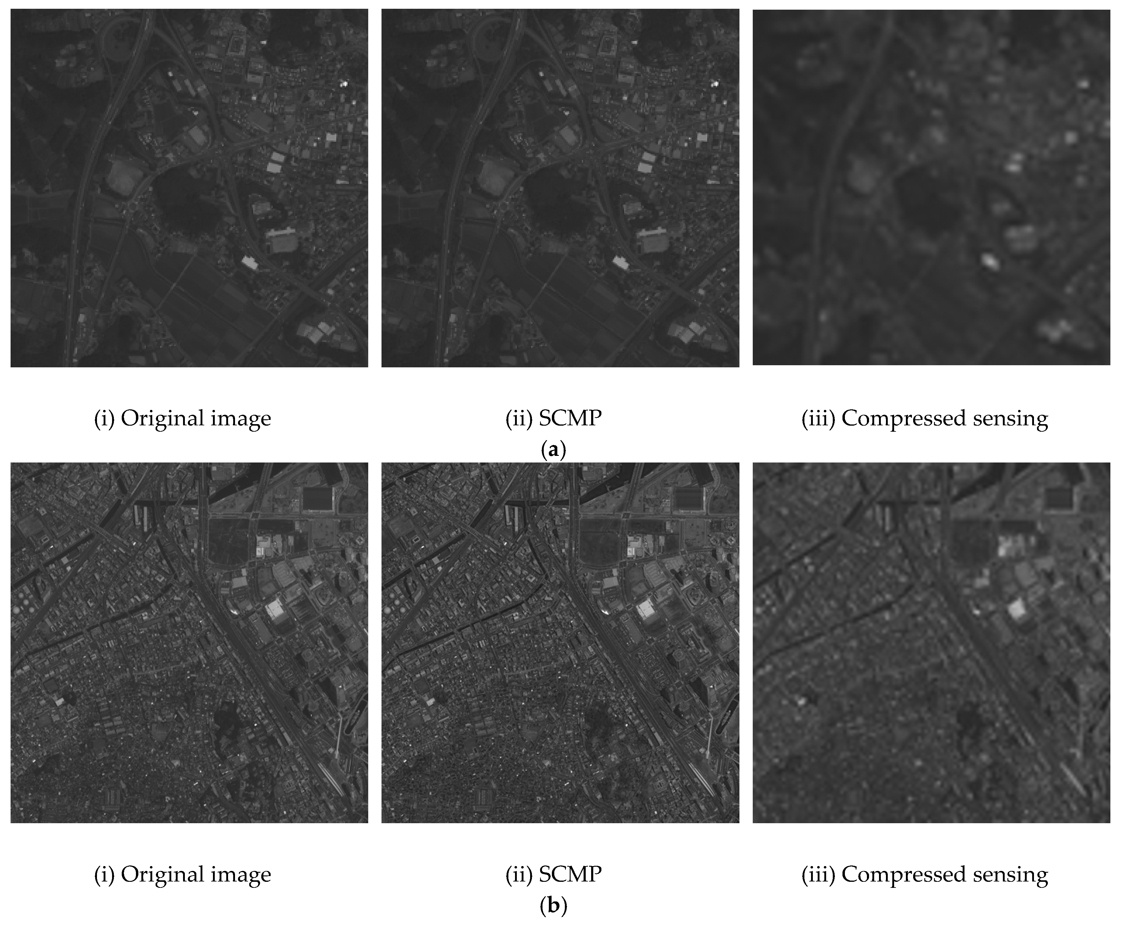
If the PAN image is corrected using the intensity obtained via SCMP, there will be little loss of spatial information. Since the intensity correction is performed appropriately on the image, the spectral distortion when using SCMP is smaller than that of the other component substitution methods. Figure 2 shows the intensity of the original RGB image, the intensity image generated by SCMP, and the intensity image obtained by CS of Nihonmatsu and Yokohama images. From this figure, it can be seen that the intensity obtained by CS had less spatial information than SCMP. In order to increase the quality of the intensity reproduced by CS using SCMP, the intensities obtained by the CS and the SCMP were combined linearly using the tradeoff parameter . In the tradeoff process, the high-resolution intensity images were obtained by SCMP and CS, and these were linearly combined by Equation (17).
2.9. Generalized IHS Method
For the fusion process, the generalized IHS method (GIHS) [5] proposed by Tu et al. was used. The intensity was calculated using Equation (6), and Equation (18) was applied to red-, green-, and blue-band RGB images.
where ,, and are the intensities of the high-resolution and low-resolution RGB images.
3. Results
3.1. Experimental Setup
3.1.1. Quality Evaluation
Visual and numerical evaluations were performed according to the Wald protocol [36]. The original MS image was used as the reference image. Correlation coefficient (CC), universal image quality index (UIQI) [37], erreur relative global adimensionnelle de synthese (ERGAS) [38], and spectral angle mapper (SAM) [39] were used for numerical evaluation. These are major evaluation criteria and used in almost all PS-related research [2]. The CC is given by
where a value closer to 1.0 implies a smaller loss of the intensity correlation and a better result. and are the total number of pixels in the entire image for each band and the number of bands in the PS image, respectively. and denote the ith pixel value of the b-band reference image and its mean value, respectively, and and denote the ith pixel value of the b-band PS image and its mean value, respectively. UIQI is an index for measuring the loss of intensity correlation, intensity distortion, and contrast distortion and is given by
where and are the standard deviation of the reference and PS images in the b-band, respectively, and denotes the covariance of the reference and PS images in the b-band. A value closer to 1.0 implies that these losses are small. The size of the UIQI sliding window was .
The ERGAS is given by
where h and l denote the spatial resolution of the PAN and MS images, respectively. The smaller the ERGAS value, the better the image quality. The SAM is an index for measuring spectral distortion and is given by
If the value is closer to 0.0, the spectrum ratio of each band is closer to the reference image.
3.1.2. Dictionary Learning
We used PAN images from the Nihonmatsu and Yokohama datasets as training images for dictionary learning. For training image and dictionary, the number of training times was 40, the number of atoms of the dictionary was 1024, and the size of each atom was . The number of patches was 6433 (Nihonmatsu) and 10,000 (Yokohama). The training dataset was a set of 1000 patches randomly selected from these patches. As the training image , a training PAN image for the high-resolution dictionary was used as the high-resolution data , and a training PAN image for the low-resolution dictionary was used as the low-resolution data . The low-resolution image was generated by downsampling and upsampling via bicubic interpolation. The sparsity regularization parameter was . The sparse representation was calculated using Equation (10) by solving the L1 norm regularized least-squares problem, and the dictionary was obtained using Equation (11) by solving the least-squares problem with quadratic constraints. We used the code provided by Lee et al. [40]. The learned high-resolution dictionaries are shown in Figure 3. For Nihonmatsu images, the dictionary created using Nihonmatsu images was used. For Yokohama images, the dictionary created using Yokohama images was used.
3.1.3. Reconstruction Process
The bicubic interpolation was used to upsample the intensity of the low-resolution RGB image. The size of the patch of the input low-resolution data was , and the overlapping region of adjacent patches was for the horizontal direction and for the vertical direction. The filter size used for the back-projection process was . The sparse representation was calculated using Equation (12) by solving the L1 norm regularized least-squares problem. We used the code provided by Lee et al. [40].
3.1.4. Coefficients for Intensity Correction
The correction coefficients estimated by SCMP are shown in Table 2. These values were used for the fusion process.
3.1.5. Tradeoff Parameter
In the tradeoff process, the intensity images obtained by SCMP and CS were combined by Equation (17) using the tradeoff parameter . The tradeoff parameter is a hyperparameter that should be determined in advance. In general, experimental validation is carried out via cross-validation when there are hyperparameters. Since we used two kinds of satellite images (Ninohmatsu and Yokohama), the value of was determined using one of these datasets, and the other dataset was processed using the determined value. In our experiment, the tradeoff parameter was determined using the correlation coefficient (CC) and ERGAS [38]. The results of applying the tradeoff parameter with a step size of 0.1 for image quality evaluation are shown in Table 3. From this result, it was found that the resolution and numerical evaluation were improved when the sum of squares of 1-CC and ERGAS was the smallest. This relationship is shown in Equations (23) and (24).
The tradeoff parameter was determined as the value that minimizes Equation (24). Figure 4 displays the results of evaluation of the intensity of RGB images with various tradeoff parameters. The red line shows Nihonmatsu, the blue line shows Yokohama, the solid line is the result of CC, and the dotted line is the result of ERGAS. Figure 5 shows three images with some tradeoff parameter values. The lower the evaluation index S, the better the visual appearance. From these results, the value that minimized was for Nihonmatsu and for Yokohama. Therefore, in the following experimetns, was used for Nihonmatsu and was used for Yokohama.
3.2. Experimental Results
Table 4 shows the effect of the back-projection (BP). The results of the intensity obtained using the sparse representation (SR) and the intensity obtained by repeating BP ten times with a size 5 filter are shown. These were compared by CC, UIQI, and ERGAS, and applying BP was better in all cases. Table 5 shows the effect of the tradeoff process (TP). The intensity images generated by SCMP, SR, and TP are shown. TP was the best in all evaluations. Table 6 shows the comparison of BP and TP. TP was better in every case.
Table 7 and Table 8 show numerical evaluations of the existing methods and the proposed method. The existing methods include fast IHS [5], Gram–Schmidt method (GS) [7], band-dependent spatial detail (BDSD) [41], weighted least-squares (WLS)-filter-based method (WLS) [42], multiband images with adaptive spectral-intensity modulation (MDSIm) [43], spectrum correction using modeled panchromatic image (SCMP) [35], image super-resolution via sparse representation (ISSR) [13] using natural images (Dict-natural) and corresponding images (Dict-self), the sparse representation of injected details (SR-D) [30], and the method of sparse representation described by Ayas et al. (SRayas) [34].
The size of the local estimation of the distinct block of BDSD was for Nihonmatsu and for Yokohama. For the ISSR settings, the training images for the dictionary included training PAN images and natural images, the number of training times was 40, the number of atoms in the dictionary was 1024, the atom size of the dictionary was , the sparsity regularization parameter was 0.1, randomly selected 1000 training image patches were used, the upscale was 4 (ratio of resolution of PAN images and MS images of IKONOS), overlap pixel of patches in the reconstruction process was in horizontal direction and in vertical direction, the size of the back-projection filter was , and the number of iterations was 10. For SR-D, high-resolution and low-resolution dictionaries were constructed from the original PAN images without training. The atom size of the high-resolution dictionary was and the overlapping areas of the adjacent atoms were ; the atom size of the low-resolution dictionary was and and the overlapping area of the adjacent atoms were .For the SRayas setting, the original IKONOS MS images were used as the training images for the dictionary, the number of training times was 20, the number of atoms in the dictionary was 4096, the size of the dictionary atom was , the sparsity regularization parameter was , the number of training image patches was 2000, the upscale was 4 (ratio of resolution of PAN images and MS images of IKONOS), , the weight of each spectral band of IKONOS was , the overlap pixel in the patch of reconstruction process was 0, the back-projection filter size was , and the number of repetitions was 20. These settings of the existing methods followed those described in the original papers except the distinct block size of BDSD. The code of Vivone et al. [2] was used for GS and BDSD, and the code of Yang et al. [13] was used for ISSR.
In Table 7 and Table 8, the highest scores are printed in bold, and the second highest scores are underlined. GS was generally not good except for the SAM of Yokohama. The results of BDSD were unremarkable but stable. SCMP was stable and gave good results. In ISSR, differences in training images had little effect on results. SRayas did not perform as well overall as ISSR and SRayas. Although some results, such as the CC of SR-D of Table 7, MDSIm of Table 8, and SAM of GS were better in part than the proposed method, in many other cases they were less accurate than the proposed method. The results of the proposed method were generally good, although there are some differences due to the tradeoff parameter.
Figure 6 shows the ranking of the quality metric of the numerical evaluations of Table 7 and Table 8, except for the proposed method. For each test, the best result was worth three points, the second-best result was worth two points, and the third-best result was worth one point. The highest score was 24 points. This figure shows that only three methods, WLS, SCMP, and the proposed method, were good for both of the images, and the proposed method got the highest score.
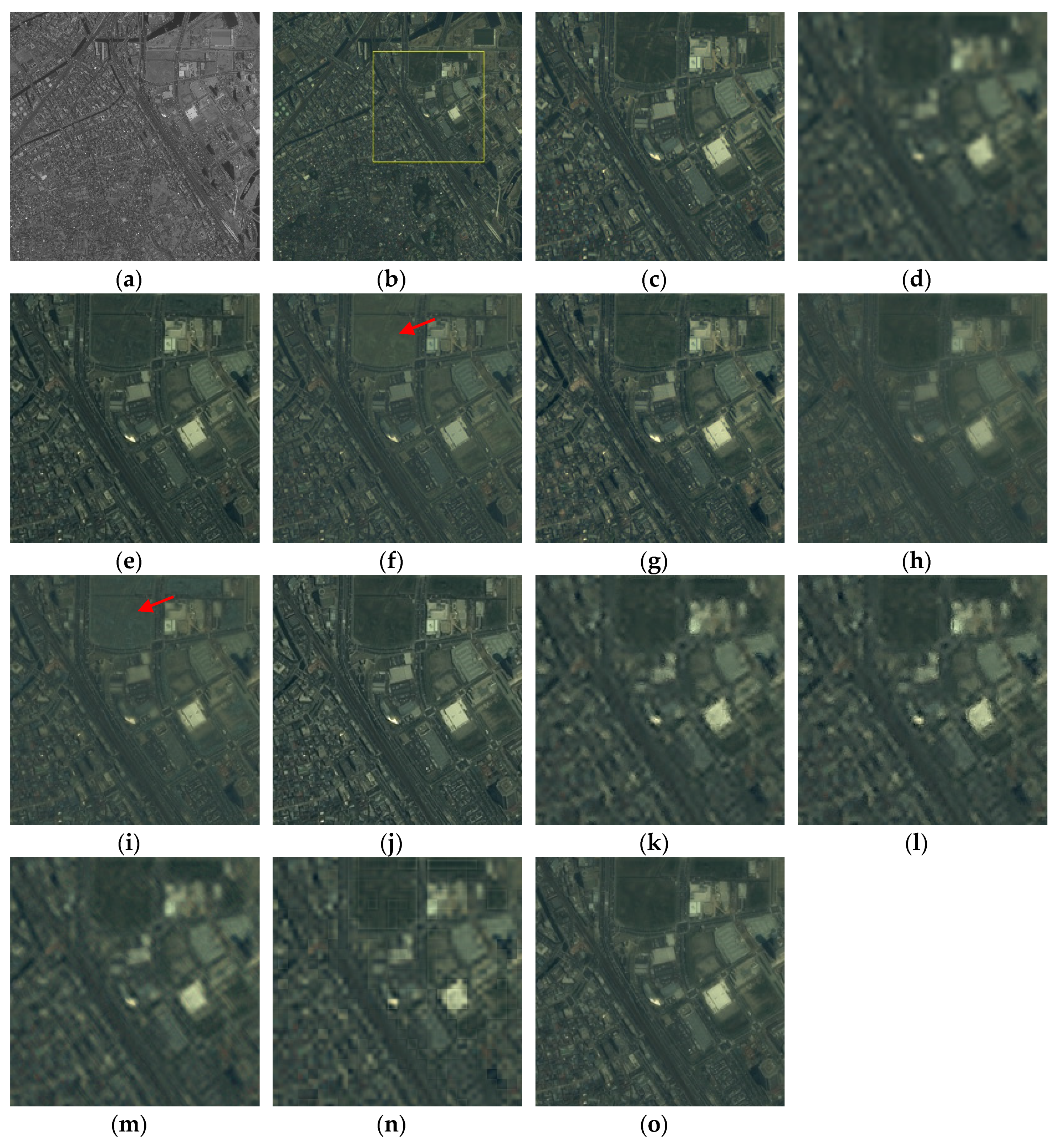
Figure 7 and Figure 8 show the reference and PS images from the Nihonmatsu and Yokohama datasets, respectively. Since the images were small, the enlarged image surrounded by the yellow frame of the original RGB image (b) is shown in (c)–(o). In Figure 7, in GS (f), the color of green was darker in the rice field area (indicated by the green arrow), while the forest area was whitish. BDSD (g) was more blurred than other images. In MDSIm (i), the color of the forest area was also whitish (indicated by the yellow arrow). In Figure 8, the vegetation area was whitish in GS (f) and MDSIm (i) (indicated by the red arrow). WLS (h) looked hazy. SR-D (m) had lower resolution than the other methods using sparse representation with back-projection. In both Figure 7 and Figure 8, the results of ISSR (k) (l) and SRayas (n) had ringing artefacts. Other images appeared to be reproduced without problems.
4. Discussion
From the results in Table 4, it was found that the back-projection (BP) was effective from the viewpoint of improving spectral distortion. From the results in Table 5, it was found that the tradeoff process (TP) is effective in improving spectral distortion. Furthermore, since the TP was better than the individual methods of sparse representation (SR) and SCMP, it was clarified that these methods complementarily improve the spectral distortion. From the results in Table 6, it was found that the TP improved spectral distortion more than BP. In the results shown in Table 7 and Table 8, the method using GIHS (WLS and SCMP) was better than the existing methods using SR. In addition, it was found that the proposed method, the linear combination of SR and SCMP, gave better results than SCMP alone. One of the problems to be solved in PS processing is the independence of the processed image. In other words, it is important to obtain stable and good results rather than obtaining good results only on a specific image. Although there are some methods shown in Table 7 and Table 8 that gave better results than the proposed method, comparing the other evaluation results shows that the results were inconsistent. The reason why the evaluation results were so different could be that these processing methods depend on the processed image.
As shown in Figure 7 and Figure 8, it was found that the reproduction of vegetation area by the GS was unstable. Since the image quality differs depending on the size of the local estimation on the distinct blocks used in BDSD, we evaluated the visibly good images with good numerical values, but the resolution of the image was low. The WLS gave good numerical results with two images, but the images were blurred. Both ISSR and SRayas using BP generated ringing artifacts. Other images seemed to be reproduced without problems in resolution and color. Among them, the proposed method gave the best results in the numerical evaluation.
In this method, resolution enhancement was achieved by using the visible and NIR regions. On the other hand, it can be applied only to the resolution enhancement of RGB images, and not NIR images.
5. Conclusions
In this paper, we proposed a method for pansharpening based on CS theory. In the proposed method, the intensity obtained from the component substitution method and the intensity obtained via the method based on CS theory are fused to reproduce the intensity close to the original. We introduced SCMP as the intensity substitution method and used the tradeoff process for image fusion. Experimental results showed that the proposed method outperformed existing methods in terms of numerical and visual evaluation. The proposed method was also effective for satellites with panchromatic sensors (observed areas are visible and NIR regions) and multispectral sensors (observed areas are red, blue, green, and NIR bands) like IKONOS.
Generally, the intensity image generated by a CS-based method is blurrier than the intensity image generated by the component substitution method, because component substitution captures the intensity of the PAN image. On the other hand, it is expected that the spectral distortion of the intensity image generated by the CS-based method will be lower than that of the image generated by the component substitution method. Since complete restoration is not guaranteed, in order to get the image close to a complete reproduction, back-projection methods can be used. However, they may cause ringing artifacts. Based on these considerations, our proposed method combines the intensities generated by the CS-based method and the component-substitution-based method via the tradeoff process instead of the back-projection to achieve both an improvement of spatial resolution and a reduction of spectral distortion. Experimental results show that the tradeoff process was more effective than the back-projection in generating a pansharpened image of which the spatial resolution was equivalent to that of the PAN image and reducing spectral distortion. Improvement of the accuracy by parameter tuning is important future work.
Author Contributions
Methodology, N.T. and Y.S.; Software, N.T.; Validation, Y.S.; Writing—Original Draft Preparation, N.T.; Writing—Review and Editing, Y.S. and S.O.; Supervision, S.O.; Project Administration, S.O.; Funding Acquisition, S.O. All authors have read and agreed to the published version of the manuscript.
Funding
This work was partially supported by the JSPS KAKENHI Grant Number 18K19772 and the Yotta Informatics Project by MEXT, Japan.
Acknowledgments
The authors thank the Japan Space Imaging Corporation and Space Imaging, LLC for providing the images.
Conflicts of Interest
The authors declare no conflict of interest.
References
- Amro, I.; Mateos, J.; Vega, M.; Molina, R.; Katsaggelos, A.K. A survey of classical methods and new trends in pansharpening of multispectral images. EURASIP J. Adv. Signal Process. 2011, 2011, 79. [Google Scholar] [CrossRef] [Green Version]
- Vivone, G.; Alparone, L.; Chanussot, J.; Dalla Mura, M.; Garzelli, A.; Licciardi, G.A.; Restaino, R.; Wald, L. A critical comparison among pansharpening algorithms. IEEE Trans. Geosci. Remote Sens. 2015, 53, 2565–2586. [Google Scholar] [CrossRef]
- Ghamisi, P.; Rasti, B.; Yokoya, N.; Wang, Q.; Hofle, B.; Bruzzone, L.; Bovolo, F.; Chi, M.; Anders, K.; Gloaguen, R.; et al. Multisource and multitemporal data fusion in remote sensing: A comprehensive review of the state of the art. IEEE Geosci. Remote Sens. Mag. 2019, 7, 6–39. [Google Scholar] [CrossRef] [Green Version]
- Pohl, C.; Van Genderen, J.L. Review article Multisensor image fusion in remote sensing: Concepts, methods and applications. Int. J. Remote Sens. 1998, 19, 823–854. [Google Scholar] [CrossRef] [Green Version]
- Tu, T.M.; Su, S.C.; Shyu, H.C.; Huang, P.S. A new look at IHS-like image fusion methods. Inf. Fusion 2001, 2, 177–186. [Google Scholar] [CrossRef]
- Zhou, J.; Civco, D.L.; Silander, J.A. A wavelet transform method to merge Landsat TM and SPOT panchromatic data. Int. J. Remote Sens. 1998, 19, 743–757. [Google Scholar] [CrossRef]
- Laben, C.A.; Brower, B.V. Process for Enhancing the Spatial Resolution of Multispectral Imagery Using Pan-Sharpening. U.S. Patent 6,011,875, 4 January 2000. [Google Scholar]
- Mallat, S.G. A theory for multiresolution signal decomposition: The wavelet representation. IEEE Trans. Pattern Anal. Mach. Intell. 1989, 17, 674–693. [Google Scholar] [CrossRef] [Green Version]
- Shensa, M.J. The Discrete Wavelet Transform: Wedding the À Trous and Mallat Algorithms. IEEE Trans. Signal Process. 1992, 40, 2464–2482. [Google Scholar] [CrossRef] [Green Version]
- Burt, P.J.; Adelson, E.H. The Laplacian Pyramid as a Compact Image Code. IEEE Trans. Commun. 1983, 31, 532–540. [Google Scholar] [CrossRef]
- Aiazzi, B.; Alparone, L.; Baronti, S.; Garzelli, A. Context-driven fusion of high spatial and spectral resolution images based on oversampled multiresolution analysis. IEEE Trans. Geosci. Remote Sens. 2002, 40, 2300–2312. [Google Scholar] [CrossRef]
- Zhang, Q.; Guo, B. Multifocus image fusion using the nonsubsampled contourlet transform. Signal Process. 2009, 89, 1334–1346. [Google Scholar] [CrossRef]
- Yang, J.; Wright, J.; Huang, T.S.; Ma, Y. Image super-resolution via sparse representation. IEEE Trans. Image Process. 2010, 19, 2861–2873. [Google Scholar] [CrossRef] [PubMed]
- Dong, C.; Loy, C.C.; He, K.; Tang, X. Image Super—Resolution Using Deep Convolutional Networks. IEEE Trans. Pattern Anal. Mach. Intell. 2016, 38, 295–307. [Google Scholar] [CrossRef] [PubMed] [Green Version]
- Masi, G.; Cozzolino, D.; Verdoliva, L.; Scarpa, G. Pansharpening by convolutional neural networks. Remote Sens. 2016, 8, 594. [Google Scholar] [CrossRef] [Green Version]
- Vivone, G.; Addesso, P.; Restaino, R.; Dalla Mura, M.; Chanussot, J. Pansharpening Based on Deconvolution for Multiband Filter Estimation. IEEE Trans. Geosci. Remote Sens. 2019, 57, 540–553. [Google Scholar] [CrossRef]
- Fei, R.; Zhang, J.; Liu, J.; Du, F.; Chang, P.; Hu, J. Convolutional Sparse Representation of Injected Details for Pansharpening. IEEE Geosci. Remote Sens. Lett. 2019, 16, 1595–1599. [Google Scholar] [CrossRef]
- Yin, H. PAN-Guided Cross-Resolution Projection for Local Adaptive Sparse Representation-Based Pansharpening. IEEE Trans. Geosci. Remote Sens. 2019, 57, 4938–4950. [Google Scholar] [CrossRef]
- Wang, X.; Bai, S.; Li, Z.; Song, R.; Tao, J. The PAN and ms image pansharpening algorithm based on adaptive neural network and sparse representation in the NSST domain. IEEE Access 2019, 7, 52508–52521. [Google Scholar] [CrossRef]
- He, L.; Rao, Y.; Li, J.; Chanussot, J.; Plaza, A.; Zhu, J.; Li, B. Pansharpening via Detail Injection Based Convolutional Neural Networks. IEEE J. Sel. Top. Appl. Earth Obs. Remote Sens. 2019, 12, 1188–1204. [Google Scholar] [CrossRef] [Green Version]
- Donoho, D.L. Compressed Sensing. IEEE Trans. Inf. Theory 2006, 52, 1289–1306. [Google Scholar] [CrossRef]
- Li, S.; Yang, B. A new pan-sharpening method using a compressed sensing technique. IEEE Trans. Geosci. Remote Sens. 2011, 49, 738–746. [Google Scholar] [CrossRef]
- Li, S.; Yin, H.; Fang, L. Remote sensing image fusion via sparse representations over learned dictionaries. IEEE Trans. Geosci. Remote Sens. 2013, 51, 4779–4789. [Google Scholar] [CrossRef]
- Jiang, C.; Zhang, H.; Shen, H.; Zhang, L. A practical compressed sensing-based pan-sharpening method. IEEE Geosci. Remote Sens. Lett. 2012, 9, 629–633. [Google Scholar] [CrossRef]
- Jiang, C.; Zhang, H.; Shen, H.; Zhang, L. Two-step sparse coding for the pan-sharpening of remote sensing images. IEEE J. Sel. Top. Appl. Earth Obs. Remote Sens. 2014, 7, 1792–1805. [Google Scholar] [CrossRef]
- Zhu, X.X.; Bamler, R. A sparse image fusion algorithm with application to pan-sharpening. IEEE Trans. Geosci. Remote Sens. 2013, 51, 2827–2836. [Google Scholar] [CrossRef]
- Zhu, X.X.; Grohnfeldt, C.; Bamler, R. Exploiting Joint Sparsity for Pansharpening: The J-SparseFI Algorithm. IEEE Trans. Geosci. Remote Sens. 2016, 54, 2664–2681. [Google Scholar] [CrossRef] [Green Version]
- Guo, M.; Zhang, H.; Li, J.; Zhang, L.; Shen, H. An online coupled dictionary learning approach for remote sensing image fusion. IEEE J. Sel. Top. Appl. Earth Obs. Remote Sens. 2014, 7, 1284–1294. [Google Scholar] [CrossRef]
- Elad, M. Sparse and Redundant Representations: From Theory to Applications in Signal and Image Processing; Springer: New York, NY, USA, 2010; ISBN 978-1441970107. [Google Scholar]
- Vicinanza, M.R.; Restaino, R.; Vivone, G.; Dalla Mura, M.; Chanussot, J. A pansharpening method based on the sparse representation of injected details. IEEE Geosci. Remote Sens. Lett. 2015, 12, 180–184. [Google Scholar] [CrossRef]
- Ghahremani, M.; Ghassemian, H. Remote Sensing Image Fusion Using Ripplet Transform and Compressed Sensing. IEEE Geosci. Remote Sens. Lett. 2015, 12, 502–506. [Google Scholar] [CrossRef]
- Zhang, K.; Wang, M.; Yang, S.; Xing, Y.; Qu, R. Fusion of Panchromatic and Multispectral Images via Coupled Sparse Non-Negative Matrix Factorization. IEEE J. Sel. Top. Appl. Earth Obs. Remote Sens. 2016, 9, 5740–5747. [Google Scholar] [CrossRef]
- Irani, M.; Peleg, S. Motion analysis for image enhancement: Resolution, occlusion, and transparency. J. Vis. Commun. Image Represent. 1993, 4, 324–335. [Google Scholar] [CrossRef] [Green Version]
- Ayas, S.; Gormus, E.T.; Ekinci, M. An efficient pan sharpening via texture based dictionary learning and sparse representation. IEEE J. Sel. Top. Appl. Earth Obs. Remote Sens. 2018, 11, 2448–2460. [Google Scholar] [CrossRef]
- Tsukamoto, N.; Sugaya, Y.; Omachi, S. Spectrum Correction Using Modeled Panchromatic Image for Pansharpening. J. Imaging 2020, 6, 20. [Google Scholar] [CrossRef] [Green Version]
- Wald, L.; Ranchin, T.; Mangolini, M. Fusion of satellite images of different spatial resolutions: Assessing the quality of resulting images. Photogramm. Eng. Remote Sens. 1997, 63, 691–699. [Google Scholar]
- Wang, Z.; Bovik, A.C. A Universal Image Quality Index. IEEE Signal Process. Lett. 2002, 9, 81–84. [Google Scholar] [CrossRef]
- Wald, L. Quality of high resolution synthesised images: Is there a simple criterion? In Proceedings of the Third Conference Fusion of Earth Data: Merging Point Measurements, Raster Maps and Remotely Sensed Images; Ranchin, T., Wald, L., Eds.; SEE/URISCA: Nice, France, 2000; pp. 99–103. [Google Scholar]
- Kruse, F.A.; Lefkoff, A.B.; Boardman, J.W.; Heidebrecht, K.B.; Shapiro, A.T.; Barloon, P.J.; Goetz, A.F.H. The spectral image processing system (SIPS)—Interactive visualization and analysis of imaging spectrometer data. Remote Sens. Environ. 1993, 44, 145–163. [Google Scholar] [CrossRef]
- Lee, H.; Battle, A.; Raina, R.; Ng, A.Y. Efficient sparse coding algorithms. In Proceedings of the 19th International Conference on Neural Information Processing Systems; Schölkopf, B., Platt, J.C., Hoffman, T., Eds.; MIT Press: Cambridge, MA, USA, 2006; pp. 801–808. [Google Scholar]
- Garzelli, A.; Nencini, F.; Capobianco, L. Optimal MMSE pan sharpening of very high resolution multispectral images. IEEE Trans. Geosci. Remote Sens. 2008, 46, 228–236. [Google Scholar] [CrossRef]
- Song, Y.; Wu, W.; Liu, Z.; Yang, X.; Liu, K.; Lu, W. An adaptive pansharpening method by using weighted least squares filter. IEEE Geosci. Remote Sens. Lett. 2016, 13, 18–22. [Google Scholar] [CrossRef]
- Yang, Y.; Wu, L.; Huang, S.; Tang, Y.; Wan, W. Pansharpening for Multiband Images with Adaptive Spectral-Intensity Modulation. IEEE J. Sel. Top. Appl. Earth Obs. Remote Sens. 2018, 11, 3196–3208. [Google Scholar] [CrossRef]
Figure 1.
Flow of the proposed method.

Figure 2.
Intensity of RGB images of (a) Nihonmatsu, (b) Yokohama. (i) Intensity of the original image, (ii) intensity of SCMP, (iii) intensity obtained via compressed sensing.
Figure 2.
Intensity of RGB images of (a) Nihonmatsu, (b) Yokohama. (i) Intensity of the original image, (ii) intensity of SCMP, (iii) intensity obtained via compressed sensing.

Figure 3.
Trained high-resolution dictionaries: (a) Nihonmatsu, (b) Yokohama.

Figure 4.
The values of CC and ERGAS obtained in the tradeoff process. CC: solid line, ERGAS: dotted line; Nihonmatsu: blue line, Yokohama: red line.
Figure 4.
The values of CC and ERGAS obtained in the tradeoff process. CC: solid line, ERGAS: dotted line; Nihonmatsu: blue line, Yokohama: red line.

Figure 5.
Comparison of intensity of RGB images against the tradeoff parameter. represents the index that determines the tradeoff parameter. (a) Nihonmatsu, (b) Yokohama.
Figure 5.
Comparison of intensity of RGB images against the tradeoff parameter. represents the index that determines the tradeoff parameter. (a) Nihonmatsu, (b) Yokohama.


Figure 6.
Scores of quality metrics.

Figure 7.
Reference and pansharpened Nihonmatsu images: (a) original PAN image (reference image), (b) original RGB image, (c) ground truth RGB image, (d) RGB image upsampled by bicubic interpolation, (e) fast IHS, (f) GS, (g) BDSD, (h) WLS, (i) MDSIm, (j) SCMP, (k) ISSR (natural images were used for training), (l) ISSR (Nihonmatsu images were used for training), (m) SR-D, (n) SRayas method, (o) proposed method .

Figure 8.
Reference and pansharpened Yokohama images: (a) original PAN image (reference image), (b) original RGB image, (c) ground truth RGB image, (d) RGB image upsampled by bicubic interpolation, (e) fast IHS, (f) GS, (g) BDSD, (h) WLS, (i) MDSIm, (j) SCMP, (k) ISSR (natural images were used for training), (l) ISSR (Yokohama images were used for training), (m) SR-D, (n) SRayas method, (o) proposed method .


Table 1.
Characteristics of the original, training, and test images of the image datasets. MS: multispectral, PAN: panchromatic.
Table 1.
Characteristics of the original, training, and test images of the image datasets. MS: multispectral, PAN: panchromatic.
| Image | Nihonmatsu | Yokohama | |
|---|---|---|---|
| Original image | PAN image | 1024 × 1024 | 1792 × 1792 |
| MS image | 256 × 256 | 448 × 448 | |
| Training image | PAN image (for high-resolution dictionary) | 256 × 256 | 448 × 448 |
| Test image | PAN image | 256 × 256 | 448 × 448 |
| MS image | 64 × 64 | 112 × 112 | |
Table 2.
The correction coefficient estimated by SCMP.
| Coefficient | Nihonmatsu | Yokohama |
|---|---|---|
| (NIR) | 0.3857 | 0.3789 |
| (Blue) | 0.2199 | 0.2549 |
| (Green) | 0.1980 | 0.1123 |
| (Red) | 0.0486 | 0.1099 |
Table 3.
CC, ERGAS, and the evaluation index S that determines the tradeoff parameter. The best values are given in bold.
Table 3.
CC, ERGAS, and the evaluation index S that determines the tradeoff parameter. The best values are given in bold.
| Tradeoff Parameter | Nihonmatsu | Yokohama | ||||
|---|---|---|---|---|---|---|
| CC | ERGAS | S | CC | ERGAS | S | |
| 0.0 | 0.899 | 2.415 | 1.186 | 0.944 | 2.393 | 0.405 |
| 0.1 | 0.908 | 2.250 | 1.016 | 0.949 | 2.148 | 0.327 |
| 0.2 | 0.915 | 2.123 | 0.892 | 0.952 | 1.996 | 0.283 |
| 0.3 | 0.920 | 2.041 | 0.815 | 0.953 | 1.961 | 0.274 |
| 0.4 | 0.922 | 2.008 | 0.783 | 0.949 | 2.050 | 0.302 |
| 0.5 | 0.921 | 2.027 | 0.800 | 0.941 | 2.248 | 0.371 |
| 0.6 | 0.916 | 2.097 | 0.873 | 0.926 | 2.529 | 0.491 |
| 0.7 | 0.906 | 2.213 | 1.011 | 0.903 | 2.870 | 0.679 |
| 0.8 | 0.891 | 2.369 | 1.228 | 0.871 | 3.251 | 0.963 |
| 0.9 | 0.871 | 2.557 | 1.550 | 0.828 | 3.660 | 1.385 |
| 1.0 | 0.846 | 2.769 | 2.000 | 0.775 | 4.088 | 2.000 |
Table 4.
Numerical evaluation of image intensities with or without the back-projection process of the intensity obtained via sparse representation. The best values are given in bold.
Table 4.
Numerical evaluation of image intensities with or without the back-projection process of the intensity obtained via sparse representation. The best values are given in bold.
| Method | CC | UIQI | ERGAS | |||
|---|---|---|---|---|---|---|
| Nihonmatsu | Yokohama | Nihonmatsu | Yokohama | Nihonmatsu | Yokohama | |
| Ideal | 1.0 | 1.0 | 0.0 | |||
| SR | 0.846 | 0.775 | 0.807 | 0.709 | 2.769 | 4.088 |
| SR+BP | 0.853 | 0.785 | 0.822 | 0.742 | 2.709 | 4.009 |
Table 5.
Numerical evaluation of image intensities obtained by SCMP, SR, and the tradeoff process. The best values are given in bold.
Table 5.
Numerical evaluation of image intensities obtained by SCMP, SR, and the tradeoff process. The best values are given in bold.
| Method | CC | UIQI | ERGAS | |||
|---|---|---|---|---|---|---|
| Nihonmatsu | Yokohama | Nihonmatsu | Yokohama | Nihonmatsu | Yokohama | |
| Ideal | 1.0 | 1.0 | 0.0 | |||
| SCMP | 0.899 | 0.944 | 0.779 | 0.915 | 2.415 | 2.393 |
| SR | 0.846 | 0.775 | 0.807 | 0.709 | 2.769 | 4.088 |
| TP | 0.920 | 0.949 | 0.825 | 0.926 | 2.041 | 2.050 |
Table 6.
Comparison of the back-projection and the tradeoff process. The best values are given in bold.
Table 6.
Comparison of the back-projection and the tradeoff process. The best values are given in bold.
| Method | CC | UIQI | ERGAS | |||
|---|---|---|---|---|---|---|
| Nihonmatsu | Yokohama | Nihonmatsu | Yokohama | Nihonmatsu | Yokohama | |
| Ideal | 1.0 | 1.0 | 0.0 | |||
| BP | 0.853 | 0.785 | 0.822 | 0.742 | 2.709 | 4.009 |
| TP | 0.920 | 0.949 | 0.825 | 0.926 | 2.041 | 2.050 |
Table 7.
Numerical evaluation of the existing methods and the proposed method by CC and UIQI. The highest scores are printed in bold, and the second highest scores are underlined.
Table 7.
Numerical evaluation of the existing methods and the proposed method by CC and UIQI. The highest scores are printed in bold, and the second highest scores are underlined.
| Method | CC | UIQI | ||
|---|---|---|---|---|
| Nihonmatsu | Yokohama | Nihonmatsu | Yokohama | |
| ideal | 1.0 | 1.0 | ||
| fast IHS [5] | 0.783 | 0.914 | 0.717 | 0.901 |
| GS [7] | 0.508 | 0.860 | 0.373 | 0.838 |
| BDSD [41] | 0.860 | 0.887 | 0.864 | 0.851 |
| WLS [42] | 0.866 | 0.884 | 0.870 | 0.759 |
| MDSIm [43] | 0.791 | 0.865 | 0.736 | 0.823 |
| SCMP [35] | 0.883 | 0.928 | 0.864 | 0.910 |
| ISSR (Dict-natural) [13] | 0.831 | 0.765 | 0.918 | 0.704 |
| ISSR (Dict-self) [13] | 0.831 | 0.759 | 0.917 | 0.701 |
| SR-D | 0.845 | 0.786 | 0.914 | 0.710 |
| SRayas [34] | 0.787 | 0.758 | 0.851 | 0.703 |
| Proposed | 0.906 | 0.937 | 0.903 | 0.918 |
Table 8.
Numerical evaluation of the existing methods and the proposed method by ERGAS and SAM. The highest scores are printed in bold, and the second highest scores are underlined.
Table 8.
Numerical evaluation of the existing methods and the proposed method by ERGAS and SAM. The highest scores are printed in bold, and the second highest scores are underlined.
| Method | ERGAS | SAM | ||
|---|---|---|---|---|
| Nihonmatsu | Yokohama | Nihonmatsu | Yokohama | |
| ideal | 0.0 | 0.0 | ||
| fast IHS [5] | 3.471 | 3.716 | 1.898 | 2.367 |
| GS [7] | 5.046 | 3.563 | 2.748 | 1.950 |
| BDSD [41] | 3.026 | 3.361 | 1.925 | 2.326 |
| WLS [42] | 2.815 | 3.816 | 1.699 | 2.123 |
| MDSIm [43] | 3.321 | 3.515 | 1.658 | 2.189 |
| SCMP [35] | 2.673 | 2.697 | 1.753 | 2.176 |
| ISSR (Dict-natural) [13] | 3.118 | 4.419 | 1.749 | 2.324 |
| ISSR (Dict-self) [13] | 3.124 | 4.474 | 1.750 | 2.331 |
| SR-D | 3.007 | 4.226 | 1.897 | 2.649 |
| SRayas [34] | 3.497 | 4.476 | 1.765 | 2.299 |
| Proposed | 2.336 | 2.424 | 1.688 | 2.159 |
© 2020 by the authors. Licensee MDPI, Basel, Switzerland. This article is an open access article distributed under the terms and conditions of the Creative Commons Attribution (CC BY) license (http://creativecommons.org/licenses/by/4.0/).
Share and Cite
MDPI and ACS Style
Tsukamoto, N.; Sugaya, Y.; Omachi, S. Pansharpening by Complementing Compressed Sensing with Spectral Correction. Appl. Sci. 2020, 10, 5789. https://0-doi-org.brum.beds.ac.uk/10.3390/app10175789
AMA Style
Tsukamoto N, Sugaya Y, Omachi S. Pansharpening by Complementing Compressed Sensing with Spectral Correction. Applied Sciences. 2020; 10(17):5789. https://0-doi-org.brum.beds.ac.uk/10.3390/app10175789
Chicago/Turabian StyleTsukamoto, Naoko, Yoshihiro Sugaya, and Shinichiro Omachi. 2020. "Pansharpening by Complementing Compressed Sensing with Spectral Correction" Applied Sciences 10, no. 17: 5789. https://0-doi-org.brum.beds.ac.uk/10.3390/app10175789
Note that from the first issue of 2016, this journal uses article numbers instead of page numbers. See further details here.