Parametric and Nonparametric PID Controller Tuning Method for Integrating Processes Based on Magnitude Optimum


1
Department of Systems and Control, Jozef Stefan Institute (JSI), Jamova Cesta 39, 1000 Ljubljana, Slovenia
2
Jožef Stefan International Postgraduate School, Jamova Cesta 39, 1000 Ljubljana, Slovenia
3
Department of E-mobility, Automation and Drives, Institute of Automotive Mechatronics, Faculty of Electrical Engineering and Information Technology, Slovak University of Technology (STU), Ilkovičova 3, 81219 Bratislava, Slovakia
*
Author to whom correspondence should be addressed.
Appl. Sci. 2020, 10(17), 6012; https://0-doi-org.brum.beds.ac.uk/10.3390/app10176012
Submission received: 4 August 2020
/
Revised: 26 August 2020
/
Accepted: 27 August 2020
/
Published: 30 August 2020
(This article belongs to the Section Electrical, Electronics and Communications Engineering)
Abstract
:Integrating systems are frequently encountered in power plants, paper-production plants, storage tanks, distillation columns, chemical reactors, and the oil industry. Due to the open-loop instability that leads to an unbounded output from a bounded input, the efficient control of integrating systems remains a challenging task. Many researchers have addressed the control of integrating processes: Some solutions are based on a single closed-loop controller, while others employ more complex control structures. However, it is difficult to find one solution requiring only a simple tuning procedure for the process. This is the advantage of the magnitude optimum multiple integration (MOMI) tuning method. In this paper, we propose an extension of the MOMI tuning method for integrating processes, controlled with a two-degrees-of-freedom (2-DOF) proportional–integral–derivative (PID) controller. This extension allows for calculations of the controller parameters from either time domain measurements or from a process transfer function of an arbitrary order with a time-delay, when both approaches are exactly equivalent. The user has the option to emphasise disturbance-rejection or tracking with the reference weighting factor b or apply two different reference filters for the best overall response. The proposed extension was also compared to other tuning methods for the control of integrating processes and tested on a charge-amplifier drift-compensation system. All closed-loop responses were relatively fast and stable, all in accordance with the magnitude optimum criteria.
1. Introduction
This paper is an extension of a previous study [1] that proposed tuning of the proportional–integral (PI) controller for integrating processes. A proportional–integral–derivative (PID) controller, in single or cascade loops and with or without derivative/integral terms, is the most commonly used control algorithm in industry [2,3,4], although several more advanced control structures have been developed. According to the authors in Reference [5], “Based on a survey of over eleven thousand controllers in the refining, chemicals and pulp and paper industries, 97% of regulatory controllers utilise a PID feedback control algorithm”. The disturbance-rejection and tracking performance depend on tuning the PID controller parameters. Despite the presence of auto-tuning algorithms [6,7], PID controllers in practice are inadequately tuned due to a lack of skill and time. According to Reference [8], “a visit to a process plant will usually show that a large number of the PID controllers are poorly tuned”. Furthermore, as stated in Reference [9], “25% of all PID controller loops use default factory settings, implying that they have not been tuned at all”.
Various tuning methods have been proposed. The first tuning rules proposed by Ziegler and Nichols [10] were followed by many tuning techniques, such as the Cohen–Coon, Chien–Hrones–Reswick, and refined Ziegler–Nichols rules. In addition to these typical tuning rules, more advanced methods have also been proposed. The latter usually use complex algorithms for the process identification [9,11,12,13,14,15,16,17,18,19]. According to the literature, the number of tuning rules for stable overdamped processes is much larger than that for integrating processes. This suggests that PID tuning for integrating processes is not an extensively studied area.
Integrating processes (IPs) involve at least one pole at their origin and are frequently encountered in industry. The main characteristics of IPs are their open-loop instability that leads to an unbounded output for a bounded input, i.e., in case of disturbances, the output drifts to extreme levels. Accordingly, the efficient IPs closed-loop control is a demanding task [20]. The IPs can be classified according to the process order. For example, typical representatives of the processes that employ pure integrator plus time-delay (ITD) transfer function models are the oil–water–gas separators in the oil industry [20], the bottom-level control in distillation columns [21], the composition control loops of high-purity distillation columns [22], heat-integrated distillation columns [23], isothermal continuous copolymerisation reactors [24], storage tanks with outlet pumps [25], vertical take-off airplanes [26], industrial injection moulding machines [27], pulp and paper plants [20], and the high-pressure steam flow to steam-turbine generators in power plants [28]. First-order integrating systems with/without delay (IFOTD) can be encountered in liquid-storage tanks [29], jacketed continuous stirred tank reactors (CSTRs) carrying out exothermic reactions [30], and paper-drum-dryer cans [31]. The most frequently encountered example of an IP with inverse response with a time-delay (INPTD) is a boiler steam drum [32].
Additionally, the open-loop responses of various industrial processes, such as liquid-storage tanks, heating boilers, liquid level systems with pumps attached to the outflow, and batch chemical reactors, are slow, with a large dominant time constant. An IP model could be used when the required settling time is shorter than the dominant time constant of a process, even if the process dynamics are inherently of a first-order lag type [18,33]. As observed in Reference [21], controller design based on IPs could provide better closed-loop performance than designs based on a first-order plus time delay process.
Many researchers have addressed controller design methods for integrating and unstable processes. Some proposed solutions are based on using a single closed-loop controller, while others employ complex control structures. Numerous IP tuning methods have been proposed so far [9,34]. These techniques can be classified according to their IP model structure, i.e., tuning methods for ITD [20,35,36,37,38,39,40,41,42,43,44,45,46,47,48,49,50,51,52,53,54,55,56,57,58,59,60,61,62,63,64,65,66], for IFOTD [8,32,34,67,68,69,70,71,72,73,74,75,76,77,78,79,80,81,82,83,84,85,86,87,88,89,90,91,92,93,94,95,96,97,98,99,100,101,102,103,104,105,106,107], for higher-order IPs with time-delay [108,109,110,111,112,113,114], and nonparametric tuning methods for IPs [1,115,116,117].
First, we present the tuning methods for ITD. Controller designs based on the IMC tuning rules for PID controllers were proposed in References [62,63,64]. In References [36,37], integral–proportional derivative (I-PD) control strategies were proposed. A two-degrees-of-freedom (2-DOF) PD-PI controller, that includes a second-order reference filter for improving tracking performance, was proposed in Reference [47]. A method for the auto-tuning of PID controllers based on closed-loop identification was proposed in Reference [38]. This method consists of the closed-loop identification of the model (after the reference or the disturbance step change), a performance assessment, and retuning of the PID controller. In Reference [39], a similar model-free PI/PID tuning method that uses a simple closed-loop reference step change (proportional control gain only) for obtaining the process model was proposed. In References [20,57], a PID controller and three-state structure for achieving a time-optimal tracking response was proposed. Since this method uses an identification technique (least-squares-based) for the calculation of the process model during steady-state changes, it is not necessary to know the process model in advance. A modified smith predictor for the control of stable, integrating, and unstable processes that consists of a 2-DOF PID controller in series with a second-order filter, defined by the dead-time and an adjustable parameter, was proposed in Reference [42]. In Reference [54], a novel approach for tuning discrete-time PID controllers with higher-order derivatives with a special focus on noise attenuation filters was proposed. These controllers offer a third degree of freedom in control design devoted to the attenuation of measurement noise. In Reference [55], two integrated tuning procedures for the joint design of a PID controller in series with an nth-order binomial low-pass filter were proposed. The proposed higher-order controller represents an intermediate step between integer and fractional-order PID controllers. Then, in Reference [56], a derivation of higher-order PID controllers by generalising the Skogestad Internal Model Control (SIMC) method [8] for analytical model-based controller tuning was proposed. In Reference [59], robust and simple analytical 2-DOF PI/PID controller tuning rules based on the multiple dominant pole method (MDPM) were proposed. The method enables calculation of controller parameters while maintaining non-oscillatory closed-loop responses without overshoots.
Note that the tuning methods for ITD can also be used for other types of IPs if the process can be modelled by the ITD model. This, for example, can be achieved by using a relay feedback identification method [37,38,41,42,43,45,46,65,101].
Next, the IFOTD tuning methods will be presented. In Reference [105], an analytical PID tuning method, where the tuning of parameters is based on maximum sensitivity (MS), was proposed. To reduce overshoots, a second-order reference filter is employed. Similar tuning rules were proposed by the same authors in Reference [106], where overshoots are reduced by cancelling some controller zeros and using fourth-order reference filtering. In Reference [97], analytical tuning rules for a 2-DOF PID controller, where overall optimal closed-loop response is obtained via two-step tuning of the closed-loop transfer function, were proposed. Controller designs based on IMC PID tuning rules were proposed in References [8,34,67,68,69,70,107]. In Reference [71], a modified IMC design based on a 2-DOF control structure that allows the separate optimisation of tracking and disturbance-rejection performance was proposed. In Reference [72], an IMC PD controller with a fractional-order filter was proposed. In Reference [73], particle swarm optimisation (PSO) and artificial bee colony (ABC) algorithms were used for PID controller tuning. Tuning rules, obtained by optimisation, were also proposed in References [74] for PI/PID, [75] for PI/PID, and [76] for I-PD. The method proposed in Reference [75] applied an additional reference filter to reduce overshoots in the tracking response. In Reference [32], analytical PI/PID controller tuning rules for IPs with non-minimum phase zeros were proposed. Calculation of the controller parameters, based on the model and the minimum Integral of the Absolute Error (IAE) criterion, was accomplished via the golden section searching algorithm. To create a 2-DOF control system, a PID controller with a unique reference filter was proposed in Reference [83]. A PID controller with set-point weighting in series with a lead/lag compensator was proposed in Reference [84]. PI/PID controller tuning rules and a method for the identification of IPs with a time-delay and inverse response from an open-loop step response were proposed in Reference [100]. In Reference [86], a methodology for the closed-loop performance assessment of a PID controller is proposed. First, the process is approximated as IFOTD from the closed-loop step response, and then the performance is evaluated by comparing it with the performance provided by the SIMC [8] tuning rule. In case the performance is not satisfactory, the PID controller is retuned using the same tuning rule. Analytical PI/PID controller tuning rules for ITD and for IFOTD based on the MDPM were proposed in Reference [102]. If the closed-loop tracking responses have higher overshoots, the method employs a 2-DOF PID controller.
Note that most tunings methods for IFOTD can also be applied to other types of IPs if the process can be modelled by the IFOTD model [8,68,69,74,75,77,78,79,80,84,87,88,91,92,93,94,95,96,98,100,106,107].
Next, we review the tuning methods for general (higher-order) IPs with time-delay. A symmetrical–optimum method for tuning PID controllers for general IPs was proposed in Reference [108]. Although this method results in higher overshoots for tracking, it is effective for disturbance rejection. A PID controller with an additional zero for the control of second-order IPs was proposed in Reference [113]. The controller tuning rules also included the controller’s sampling time, Ts. In Reference [109], a new classification for a large class of stable, oscillatory, integrating, and unstable processes with or without time-delay was proposed. This was done by using the proposed ρ–φ parameter plane, defined by the normalised gain, ρ, and the angle, φ, of the Nyquist curve slope at the process’ ultimate frequency. Next, PID controller tuning formulae for obtaining the desired performance/robustness trade-off in the chosen region of the ρ–φ parameter plane are proposed.
Nonparametric tuning methods are data-based, i.e., they directly exploit the closed- or the open-loop process datasets, without the need for a process model. This is an attractive approach for alleviating the drawbacks of process–model mismatches. A PI/PID controller tuning method that enables specification of the desired closed-loop transfer function for disturbance-rejection, while tracking, using PID controllers, can be independently improved with set-point weighting, was proposed in Reference [115]. A tuning method for PI and PID controllers, based on an extended relay feedback procedure, was proposed in Reference [117].
Most of the proposed tuning methods offer limited range of IP models, require an accurate IP model, or optimisation of the controller parameters. Additionally, some methods do not give satisfactory closed-loop responses, and some others may not work with parameter uncertainty (stability/robustness).
Magnitude optimum (MO) is a controller tuning rule based on the optimal closed-loop frequency response [118,119,120]. The closed-loop performance for tracking and disturbance-rejection is usually fast and without oscillations [121]. By using a nonparametric time domain approach with multiple integrations of the process signals, the applicability of the MO method has been extended. This extension is called the magnitude optimum multiple integration (MOMI) method [122] and retains all the advantages of the MO method. Additionally, this extension offers an extraction of the necessary data from a simple time domain experiment [121,122].
When using a one-degree-of-freedom (1-DOF) controller structure, the MO criteria result in the integrating gain of the PID controller equal to zero. Since the resulting PD controller cannot reject input disturbances, the original MOMI tuning rule cannot be used for IPs. However, in Reference [1], Kos et al. proposed an extension of the MOMI tuning method for IPs controlled by a 2-DOF PI controller.
In this paper, an extension of the MOMI tuning method for integrating processes, controlled with the 2-DOF PID controller, is proposed. Additionally, to achieve the best overall closed-loop responses (the optimal tracking and disturbance-rejection), two reference filter structures are proposed. The proposed method is nonparametric, meaning that it does not require an explicit process model, which is an attractive approach for alleviating the possible problems related to the process–model mismatch. The controller parameters can be calculated from the process’ closed- or open-loop time response or from the arbitrary process transfer function with a time-delay. Both approaches are equivalent. Furthermore, the user has the additional option to emphasise disturbance-rejection or tracking with the reference weighting factor b or to simply use the reference filter for the best overall responses.
The content of this paper is organised as follows. First, the MOMI tuning method and the PID extension for IPs are presented. Section 3 presents two reference filter structures for achieving the best overall closed-loop responses. Section 4 provides examples of diverse IP models and a comparison between the proposed MOMI PID and MOMI PI extension for the IPs and between the proposed extension with and without the reference filter. Section 5 assesses the stability and robustness of the proposed tuning method. In Section 6, the proposed method is compared with other IPs tuning methods. A real-time experiment in the time domain on a charge-amplifier drift-compensation system is outlined in Section 7.
2. MOMI Tuning Method for Integrating Processes
2.1. Closed-Loop Configuration and Magnitude Optimum Multiple Integration
In this section, we present a method for the non-parametric identification of the process using so-called characteristic areas (process moments) [18]. These areas can be identified from a closed- or open-loop time response (in the time domain) or directly from an arbitrary rational transfer function with a pure time-delay (in the frequency domain). It is worth mentioning that both approaches (time and frequency domain) are equivalent. Later, the characteristic areas will be used for the calculation of the controller and the reference filters’ parameters.
Figure 1 shows a 2-DOF controller in a closed-loop configuration with a process. Signals u, d, y, and r represent the process output, input disturbance, controller output, and controller reference, respectively.
The process is defined by the stable transfer function:
where the process time-delay is represented by Tdelay. As stated in Reference [119], “one possible design aim is to maintain the closed-loop magnitude response curve as flat and as close to unity for as large a bandwidth as possible” (see Figure 2). Thus, the goal is to find a controller that has a low-frequency closed-loop response as close to unity as possible [121].
This approach is called modulus optimum, Betragsoptimum, or magnitude optimum (MO), and results in a relatively optimal closed-loop time response for a majority of process models, when considering the speed of its response and robustness [121].
With a 2-DOF controller (in Figure 1), the closed-loop transfer function becomes
The controller is configured so that
is fulfilled for as many k as possible [119,122]. Equation (3) is thus easily fulfilled. If the controller structure contains integral term and the closed-loop response is stable, the steady-state control error is zero; hence, Equation (3) holds. The number of satisfied conditions in Equation (4) is correlated to the number of controller parameters (controller order). For the PID controller, kmax = 3.
Let us define the closed-loop transfer function by the following equation:
Then, the following conditions must be satisfied to fulfil Expression (4) [121]:
For the calculation of the PI controller parameters, the first two equations in Condition (6) should be fulfilled, and for the calculation of the PID controller parameters, the first three equations in Condition (6) should be fulfilled.
To simplify further derivations, Process (1) is developed into an infinite Taylor series [122]:
where Ai represents the “characteristic areas” of the process [121], which can be expressed by Process Parameters (1) [119]:
This means that the characteristic areas can be obtained directly from the process transfer function. Additionally, the characteristic areas can also be calculated in the time domain, i.e., from the process time response. To this end, the steady state of the process should be changed first. Then, the multiple integrations of the process input (u(t)) and output (y(t)) signals can be calculated [119,122]:
where u0 represents the normalised process input signal, and
The characteristic areas are expressed as follows:
Note that and that A0 equals the process steady-state gain, KPR. In practice, the integration in Expression (9) can end when the process signals settle. Thus, Expression (9) can be recursively and simply calculated, therefore the process Model (1) is not needed. Therefore, using the characteristic areas, the process can be easily parameterised from any change in the process steady state [121].
In practice, certain rules need to be followed to accurately calculate the areas from the process response corrupted by noise. A few practical guidelines for calculating the characteristic areas from the process time responses in practice, including the high-frequency process noise, are provided in Reference [123]. As will be shown in Section 7, the method was also tested on a real process with present noise. Moreover, the proposed method for the PI controller [1] has also been tested on several processes with measurement noise. In all the mentioned tests, it was shown that the calculated areas and, therefore, the controller parameters, are not extensively sensitive on high-frequency process noise. However, the method still requires deeper noise analysis to be carried out in the future.
2.2. Extension to Integrating Processes
Figure 4 presents the closed-loop system with a 2-DOF PID controller. Signals y, d, u, and r represent the process output, disturbance, controller output, and controller reference, respectively. Parameters b and c are the proportional and derivative weighting factors, while KD, KP, KI, and TF are the derivative gain, proportional gain, integral gain, and filter time constant, respectively.
The controller presented in Figure 4 is defined by the following transfer functions:
To simplify the derivations, c = b is chosen. Thereafter, this controller will be denoted PIDb. While the controller filter
is actually part of the PIDb controller transfer function. To simplify the derivation of the PIDb controller parameters, the controller filter is considered part of the Process (1). Therefore, the aforementioned filter must be added to Expression (1) every time the PIDb controller parameters are calculated with the final formula.
The controller filter is used for reduction of the controller’s output high-frequency noise. The controller’s high-frequency gain equals to [18]. Besides defining the controller filter time constant in advance, it can also be calculated based on the desired high-frequency gain as follows:
Initially, the controller parameters (including derivative gain KD) should be calculated with TF = 0. Next, the controller parameters can be calculated again by applying Equation (14). The procedure can be repeated until the TF value settles. In practice, up to three iterations are usually sufficient.
In the following derivation, the PIDb controller parameters will be calculated. The IP has been modelled by the transfer Function (1). Next, Process (7) and the Controller (12) transfer functions are inserted into a closed-loop transfer Function (2). In this way, the following closed-loop transfer Function (5) parameters are obtained:
To simplify the derivation of the PIDb controller parameters, in the next step, all closed-loop transfer function parameters, represented by Expressions (15) and (16), are divided by A0KI. Consequently, the following closed-loop transfer function Parameters (5) are obtained:
where
For calculation of the three PIDb controller parameters, the first three equations in Condition (6) should be solved. The first condition of Expression (6) gives the following result:
and the second condition in Expression (6) provides the following result:
The third condition of Expression (6) gives the following fourth-order polynomial:
where
To calculate the PIDb parameters, the integral time constant TI, represented by Expressions (22) and (23), should be solved first. The correct result is the highest positive real number. In the next step, integral gain, KI, should be calculated using Equation (21). In the last step, the proportional, KP, and derivative, KD, gains can be calculated using the following expression:
Since calculating the PIDb controller parameters requires solving the fourth-order polynomial, the final derivation of the tuning formula is not presented. Regardless, the tuning formula remains analytical. To facilitate the implementation of the proposed tuning method and save the reader’s time and effort, all MATLAB files used for the calculation of the PIDb parameters are available online in Reference [124].
Remark 1.
Weighting factor b influences the disturbance-rejection and tracking performance. When b approaches 1, the integral gain KI (21) approaches 0 [1]. For b = 1, we obtained the following PID controller:
Thus, we obtained a PD controller that cannot reject the process input disturbances. For this reason, increasing the value of weighting factor b degrades the disturbance-rejection performance. In practice, the value of b should be limited within the interval 0 < b < 0.9 [1]. An illustrative example showing the tracking and disturbance rejection performance and its relationship to factor b is presented in Section 2.3.
Remark 2.
The PIDb controller parameters calculated by Expressions (21) and (24) result in stable and fast closed-loop responses for most IP models. However, the closed-loop stability of an arbitrary process model is still not guaranteed. Section 5 provides additional information on closed-loop stability and robustness.
As explained in Section 2.1, the characteristic areas A0 to A4 can be obtained directly from the process transfer function or calculated from the process time response when changing the process steady state. The following steps are required for PIDb controller tuning:
- Choose the appropriate filter time constant, TF, of the PIDb controller.
- Determine the characteristic areas A0–A4. If the process is given in a Laplace form, use Expression (8) (frequency domain). Otherwise, change the steady-state of the process, capture the controller and process output signals, and calculate the characteristic areas using Expressions (9)–(11) (time domain). The initial values of the controller and the process output signals (before the first change of the process input signal) can be approximated from the measurements. Do not forget to add the filter time constant, TF, to the process transfer Function (1) before calculating the areas. If the time domain approach is used, use the first-order filter with a time constant that equals TF to filter the process output signal.
- Select the reference weighting factor b. As seen in Remark 1, the recommended values are 0 ≤ b < 0.9.
- Use Expressions (21) and (24) to calculate the PIDb parameters KP, KI, and KD.
Remark 3.
For obtaining the a-priori chosen high-frequency controller gain KHF, the exact value of TF can be calculated according to the procedure described below Equation (14).
2.3. Illustrative Example
The following second-order delayed IP is chosen to illustrate the proper design:
First, the PIDb controller filter time constant TF = 0.01 s is added to Process (26). Using Expression (8), the following characteristic areas are calculated from Process (26)’s transfer-function with a filter:
In the next step, using Expressions (21) and (24), the PIDb controller parameters are calculated for different values of reference weighting factor b. The calculated parameters presented in Table 1 are applied to the PIDb controller. The closed-loop responses (reference step change r = 1 and input disturbance step change d = 1) are shown in Figure 5.
As seen in Figure 5, the reference weighting factor b has a significant impact on the closed-loop responses. Tracking (reference-following) performance is improved at higher values of b. Thus, in cases where good tracking is desired, choose a value of b ≥ 0.5. However, high values of b degrade the disturbance-rejection performance, i.e., the disturbance-rejection performance seriously deteriorates at b > 0.7. The most effective disturbance-rejection is obtained with b ≤ 0.5. An acceptable compromise between both tracking and disturbance-rejection seems to be b = 0.5.
3. Optimal Tracking and Disturbance-Rejection
Besides using the reference-weighting parameter b (note that c = b), the closed-loop tracking response can be improved by applying a reference filter. The main advantage of using a reference filter is that such a filter can substantially improve the tracking response without deterioration of the disturbance-rejection response (the optimal one, as calculated with b = 0). In this way, the best overall response can be achieved. A similar approach was proposed in Reference [125] for non-integrating processes. The filter (GF) in the closed-loop configuration with the PID controller (GC) and the process (GP) is shown in Figure 6. For the proposed tuning method with a reference filter, the controller parameters are calculated for the weighting factor b = 0 to retain the good disturbance rejection properties, while the controller structure is 1-DOF PID (b = 1).
Here, two controller structures with reference filters are proposed according to the following filter order: The PID controller with the second-order filter (PIDf2) and the higher-order filter (PIDfh).
3.1. The Second-Order Filter
The closed-loop transfer function GCL from the reference to the process output is the following:
The purpose of the reference filter GF is to make the reference following transfer Function (28) as closely as possible to the desired function with the PD controller (b = 1):
where KP1 and KD1 represent the controller Parameters (25) of the PD controller. The structure of reference filter GF is chosen as follows:
The denominator of the Filter (30) is chosen to cancel the controller zeros in the closed-loop transfer Function (28), similar to the approach proposed by Medarametla and Manimozhi [106]. The numerator of the filter (parameters bF1 and bF2) is then calculated by equating the first two characteristic areas (A0 and A1) of the closed-loop transfer Function (28) (using Expression (8) with GCL instead of GP1 in the Expression (7)) with the equivalent areas of the desired closed-loop transfer function GCL1 when using the PD Controller (29). The following filter parameters are thus obtained:
3.2. The Higher-Order Filter
To achieve an even faster closed-loop tracking response than that with the PD Controller (25), a higher-order filter can be applied. Here, the calculation of the filter parameters is based on the process model. However, this does not mean that the main advantage of the proposed tuning method is lost (note that the process model is not required for the calculation of the controller parameters). Instead, the process model will be estimated from the characteristic areas, where the only required parameter from the user is the estimated process time-delay, which can be easily acquired in practice from the process time-response. The chosen process model is a second-order process with zero and the estimated pure time-delay
where Tdm and KM represent the process time-delay and steady-state gain, respectively. Note that the model parameters (except for the estimated time-delay, Tdm) can be calculated directly from the equations for the characteristic areas A0 to A3 (8):
For minimum-phase processes, the model transfer function can be simplified by setting b1m = 0, which in turn simplifies the identification procedure. Namely, all the process model parameters, including the process time-delay Tdm, can be calculated analytically [126] from Expression (8):
where Tdm is calculated from the above third-order equation. The result (among three solutions) is the lowest positive real number.
The closed-loop transfer function from the reference to the process output, when process GP is replaced by the process model GM, is the following:
We can now define the desired closed-loop transfer function as follows:
where
TCL is the desired closed-loop time constant. Note that parameter TCL is related to the speed of the response of the PD controller, so it will be automatically calculated, and no user input is required. Let us define the closed-loop time constant TCL0 equal to the integral of the control error at the unit stepwise reference change:
where KP1 is the proportional gain of the PD controller. The desired closed-loop time constant TCL is then defined as follows:
where parameter KCL defines the speed-up coefficient of the closed-loop time constant in relation to that obtained with the PD controller. According to the results of the experiments using different process models, the parameter KCL = 3 is found to be a good compromise between tracking speed and robustness.
To equate Expressions (35) and (36), the time-delay in the denominator of (35) is expressed by the second Pade’s approximant:
By Equations (35) and (36) and taking into account (40) in the denominator of (35), the following reference filter transfer function is obtained:
where n is calculated from Expression (37).
Parameters bF1 to bF5 in the numerator are calculated from the denominator of the closed-loop transfer Function (35) without the reference filter GF:
by equating the terms with the same power of the Laplace variable s. The resulting parameters are the following:
where TF is the controller filter time constant.
Remark 4.
The reference filter is not in the feedback part of the closed-loop system transfer function. Therefore, as long as the reference filter is stable, it does not change the stability of the entire closed-loop system. By observing the higher-order reference filter Denominator (41), it can be seen that majority of the filter poles are on the left-hand side of the complex plane. The only part of the denominator filter that might become unstable is the following term:
By using simple derivation, it can be shown that the mentioned Term (44) is stable if all of the controller gains are of the same sign. The same applies for the second-order reference Filter (30), which also contains the same Term (44).
To facilitate the implementation of the proposed reference filters and to save the reader’s time and effort, all MATLAB files for the calculation of the second- and higher-order filter parameters are available online in Reference [124]. Note that, as with the MOMI tuning method, the reference filter parameters can be calculated from the measured characteristic areas, which can be acquired from the process steady-state time response.
4. Illustrative Examples
The proposed method (PIDb, PIDf2, and PIDfh) was tested on some process models. Additionally, it was compared to the MOMI PI controller tuning method for integrating processes [1].
4.1. MOMI PIDb Controller
In this section, the proposed method without a reference filter has been tested on some common process models. The chosen IPs were a delayed second-order process, a pure integrator plus time-delay process, a fourth-order process, and a non-minimum phase process. These processes are represented by the following transfer functions:
First, the a-priori chosen PID controller filter time constant TF = 0.01 s was added to Processes (45). Then, using Expression (8), the characteristic areas A0 to A4 were calculated. The values are presented in Table 2.
The PIDb controller parameters for different values of b (b = 0, b = 0.5, and b = 0.7) were calculated from Equations (21) and (24) using the calculated characteristic areas from Table 2. The calculated parameters for all selected IP models are presented in Table 3.
The calculated controller parameters were applied to a PIDb controller. Figure 7, Figure 8, Figure 9 and Figure 10 show the closed-loop responses for the input disturbance step change (d = 1) and for the reference step change (r = 1). From the experimental results, it can be seen that the proposed tuning method provided relatively fast and stable closed-loop responses. Additionally, all responses were highly damped with only minor overshoots. The closed-loop responses are in accordance with the magnitude optimum criterion. Exceptions include the sluggish disturbance-rejection responses at b = 0.7. As expected, the best tracking performance was achieved with b = 0.7, and the best disturbance-rejection performance was achieved with b = 0 (see also the illustrative example in Section 2.3).
The Bode plots of the closed-loop amplitude gains (between the reference and the process output) are shown in Figure 11. This figure shows that all the processes have a flat amplitude low-frequency response, which is in accordance with the MO criterion (see Figure 2). Moreover, the reference weighting factor b has an influence on the closed-loop bandwidth, i.e., the closed-loop bandwidth decreases by decreasing factor b. Therefore, the tracking performance improves by increasing factor b, which is in accordance with the findings in Section 2.3 (illustrative example).
4.2. Comparison with the MOMI Tuning Method for PI Controllers
The performance of the proposed MOMI PIDb method was compared with the MOMI PI method for IPs [1] on four process models. Note that this PI controller also includes the reference weighting factor b on the proportional term. The following IPs were chosen:
First, the parameters for the PI controller were acquired. To that end, the characteristic areas A0–A2, presented in Table 2, were calculated. The PI controller parameters for two different values of b (b = 0 and b = 0.5) were then calculated via the following Equations [1]:
using the calculated characteristic areas from Table 4. The calculated PI controller parameters for all four IP models are presented in Table 5.
Next, the parameters for the PIDb controller were acquired. Note that the a priori chosen PIDb controller filter time constant TF = 0.01 s (13) was added to Processes (46). Then, by using Expression (8), the characteristic areas A0 to A4 presented in Table 6 were calculated. The PIDb controller parameters for different values of b (b = 0 and b = 0.5) were calculated from Equations (21) and (24) using the calculated characteristic areas from Table 6. The calculated PIDb controller parameters for all four IP models are presented in Table 7.
The calculated controller parameters presented in Table 5 and Table 7 were applied to the PI and PIDb controllers. Figure 12, Figure 13, Figure 14 and Figure 15 show the compared closed-loop responses for the input disturbance step change (d = 1) and for the reference step change (r = 1). This comparison shows the superior tracking and disturbance-rejection performance of the PIDb controller.
4.3. MOMI PID with Reference Filters
Besides using the reference weighting factor b, the 2-DOF controller can also be realised via a PID with an additional reference filter (see Section 3).
Here, the proposed PIDb controller will be compared to the proposed PIDf2 and PIDfh controllers. For this purpose, the same process models used in Section 4.1 (45) are used here.
The chosen controller filter time constant was the same as before (TF = 0.01 s). The characteristic areas A0 to A4 are given in Table 2. The PIDb controller parameters calculated using various values of b are given in Table 3. Note that, for the PIDf2 and PIDfh controllers, the proportional, integral, and derivative gains for PIDb with b = 0 were used.
The reference filter parameters for the PIDf2 and PIDfh controllers were calculated from Equation (31) (PIDf2 controller) and Equation (43) (PIDfh controller) using the calculated characteristic areas from Table 2 and the calculated PIDb controller parameters (b = 0) from Table 3. The values of the PD controller parameters, the estimated second-order process model parameters, and the chosen speed-up coefficient of the closed-loop time constant are shown in Table 8. The calculated reference filter parameters for the PIDf2 and PIDfh controllers are given in Table 9 and Table 10, respectively.
Figure 16, Figure 17, Figure 18 and Figure 19 show a comparison of the closed-loop responses for input disturbance step change (d = 1) and the reference step change (r = 1). This comparison shows the superior tracking abilities of the PIDf2 and PIDfh controllers. The tracking speed of the PIDfh controller is considerably greater than that of the other methods. Note that the disturbance-rejection performance of the PIDf2 and PIDfh controllers is equal to that of the PIDb controller with b = 0. On this basis, we can conclude that the proposed tuning method for the PIDf2 and PIDfh controller gives the best overall response (optimal tracking and disturbance-rejection).
5. Stability and Robustness
In general, the stability of the closed-loop system can be calculated from the roots of the closed-loop transfer function denominator (denCL):
where
Clearly, the denominator consists of a pure time-delay, which complicates the stability analysis. The time-delay in denCL (49) can be developed into an infinite-order Taylor series. However, the analysis of infinite-order series using, e.g., the Routh–Hurwitz stability criterion, is far from straightforward and outside the scope of our research.
However, the stability and robustness of closed-loop systems can be tested on process models that cover most of the integrating processes in various industries. One such process model is the second-order integrating process with a time-delay:
The process GP (s) (50) also covers pure time-delay and the first-order integrating processes. The stability and robustness of the closed-loop system will be tested with different ratios of Tdelay/a1 and factor α. Note that this process has real poles only when α ≤ 0.25.
When choosing the PIDb controller reference weighting factor b = 0, the closed-loop system is stable for any positive values of α and Tdelay. The system is also stable for all the processes with real process poles for b = 0, b = 0.5, and b = 0.9. As shown by Figure 20, increasing factor b has a negative impact on system stability. This system is stable for any time-delay with b = 0.5 if α ≤ 1.5, and α ≤ 1.05 with b = 0.9. The overall stability improves by increasing the time-delay or decreasing b and the factor α.
The closed-loop system’s robustness was tested by measuring the maximum sensitivity function, MS [1,11,127]. A higher value of MS indicates lower system robustness since the open-loop transfer function GPGCY is closer to the critical point (−1 + 0i). The most common values of MS for integrating processes are usually higher than those for non-integrating processes [11] and are typically between 1.7 and 3.
The maximum sensitivity functions are calculated for different values of b (0, 0.5, and 0.9) and are shown in Figure 21, Figure 22 and Figure 23. Note that the MS values for processes with real poles are below 3.15 for b = 0, below 2.45 for b = 0.5, and below 1.85 for b = 0.9. The expected robustness of the closed-loop system for the processes with real poles is, therefore, satisfactory and relatively high. Processes with complex poles result in lower robustness, which is expected.
The robustness of the proposed tuning method (PIDb and PIDfh controller) is next studied for the following process model:
First, the PIDb controller filter time constant TF = 0.01 s was added to Process (51). Using Expression (8), the following characteristic areas were calculated from Process (51)’s transfer function:
In the next step, the PIDb controller parameters for reference weighting factors b = 0.5 and b = 0 were calculated using Expressions (21) and (24):
Additionally, the parameters of the PIDfh controller reference filter were calculated using Expression (43) (for chosen KCL = 3):
The calculated parameters were applied to the PIDb and PIDfh controllers. The robustness was studied by assuming a ±10% change in the Process (51) steady-state gain and time-delay. Figure 24 and Figure 25 show the corresponding responses for the input disturbance step change (d = 1) and the reference step change (r = 1) for the PIDb controller with b = 0.5 and for the PIDfh controller, respectively.
As can be seen from the process output responses, a change in the process gain or time-delay does not deteriorate the tracking or disturbance-rejection responses. Nevertheless, the PIDfh controller seems to be slightly more sensitive to process perturbations (especially the increased process gain).
6. Comparisons with Other Methods
As far as we know, no other tuning method for IPs offers tuning based on both the measurement of a simple process open- or closed-loop time response in the time domain and a general process transfer function with an arbitrary order with time-delay. This represents a significant advantage over alternative tuning methods for PID controllers.
Nevertheless, in this section, the results of the simulations of five different IP models that often appear in the literature are compared with those of other PID tuning methods for IPs. Notably, the selected tuning methods are not model-free controller tuning methods. Some methods cannot be used on arbitrary IP models. However, all the chosen methods provide analytical tuning formulas for the calculation of the controller parameters.
The proposed tuning method for the PIDf2 and PIDfh controllers was compared to five other methods [18,77,97,103,106]. The first method is Ali and Majhi’s method [77] (hereafter denoted as Ali–Majhi) for 1-DOF PID controllers. This method achieves optimal load disturbance-rejection for IPs with Integral of the Squared Error (ISE) criterion minimisation with Nyquist curve constraints, e.g., the slope has a specified inclination at the gain crossover frequency. The second method is that of Taguchi and Araki [97] (hereafter denoted as Taguchi) for 2-DOF PID controllers. This method optimises the settling time while keeping the overshoot under 20%. The third one is Medarametla and Manimozhi’s method [106] (hereafter denoted as Medarametla), which is based on the loop sensitivity transfer function. This controller consists of a 1-DOF PID controller with a second-order Lead/Lag filter and a fourth-order reference filter that cancels some controller zeros. The fourth method is that of Anil and Padma Sree [103] (hereafter denoted as Anil–Padma), which employs a pole-placement strategy, and the tuning parameter is the MS. The controller consists of a 2-DOF PID controller with a first-order Lead/Lag filter. The last is Åström and Hägglund’s method [18]. This method is based on selecting a maximal sensitivity value MS = 1.4 (hereafter denoted as Åström 1.4) or MS = 2.0 (hereafter denoted as Åström 2). The method employs a 2-DOF PID controller. Note that these methods employ different controller structures.
The closed-loop tracking (r = 1) and disturbance-rejection (d = 1) responses were measured on all five process models. In all cases, the a priori chosen controller filter time constant was , with the exception of the Ali–Majhi method, where the controller filter time constant was set to the proposed value of .
The calculated controller parameters (for all presented tuning methods and the proposed tuning method) for all five IP models are found in the Tables S1—S10 of the Supplementary Materials Section 1.
The tracking and disturbance-rejection performance of the tuning methods can be evaluated by the following criteria:
where RVy is the relative variance of the process output signal:
and y1 and y2 are the first and the second extrema of the process output signal. The RVy for tracking becomes 1 for a monotone process output signal. For any other response (overshoots, undershoots, or oscillations), the value will increase. The RVy for disturbance becomes 1 for the process output signal, which has only one maximum and one minimum. This is an ideal disturbance-rejection response. Since the RVy measure favours monotonic responses, while IAE favours fast responses, the combined measure () offers the best compromise between speed and monotonicity.
The RVy measures are based on the TV0y and TV2y measures introduced in References [48,128]. Note that the TV0y and TV2y measures are 0 for monotone responses (or responses with one maximum and one minimum). Since we multiply the RVy with IAE, the RVy is modified to give values of 1 instead of 0 under ideal circumstances.
Like , the IAT2E measure favours fast and non-oscillatory responses.
Note that the measurements of the criteria were taken after the process output completely settled, meaning that the simulations were longer than those shown for the closed-loop responses below.
Case 1
The next pure integrator plus time-delay is chosen as
The tracking and the disturbance-rejection closed-loop responses between the aforementioned tuning rules are compared in Figure 26 and Figure 27. The criteria values of the tuning rules are presented in Figure 28.
According to the IAE criterion, the proposed controllers ranked first, and according to the IAT2E criterion, they ranked first and third in tracking performance. The proposed PIDfh controller also ranked first for the criterion. The Ali–Majhi method showed a large overshoot, and the Åström 2 method exhibited a somewhat oscillatory response.
The Taguchi method obtained the lowest criteria for disturbance-rejection. The proposed tuning method was ranked second. However, the Taguchi method exhibited a slightly oscillatory response.
Concerning sensitivity MS, Anil–Padma and Medarametla suggested MS = 2 for processes without zero, while the proposed method gave values below 3.3.
Case 2
The following slightly delayed first-order process is chosen:
Figure 29 and Figure 30 compare the closed-loop tracking and disturbance-rejection responses for all mentioned tuning rules. The criteria values of the aforementioned tuning rules are presented in Figure 31.
The lowest criteria for tracking was obtained by the proposed PIDfh controller. The Medarametla method ranked second, and the PIDf2 ranked third. The Taguchi and the Ali–Majhi method exhibited a somewhat oscillatory response.
For the disturbance-rejection performance, the criteria favoured the Medarametla method. However, the proposed method was ranked second, close to Medarametla. Like tracking, the Taguchi and Ali–Majhi methods exhibited oscillatory responses.
Concerning sensitivity MS, Anil–Padma and Medarametla suggested MS = 2 for processes without zero, while the proposed method gave values below 3.
Case 3
The next second-order process with time-delay is chosen:
The tracking and disturbance-rejection closed-loop responses between the tuning rules are compared in Figure 32. Some methods are missing because they are not suitable for second-order process models. The criteria values of the tested tuning methods are presented in Figure 33.
The tracking criteria gave the lowest values for the proposed controllers. The Åström methods ranked second. Again, the Taguchi method exhibited an oscillatory response.
Similarly, the lowest criterion for disturbance-rejection was given for the proposed controllers, with the Åström 2 method close behind.
Concerning sensitivity MS, the proposed method gave values below 2.5. As expected, the MS values for the Åström methods were lower since that tuning method is based on MS values.
Case 4
The following high-order non-minimum phase process is chosen:
An experiment using this process was already carried out by Medarametla and Manimozhi [106] (Medarametla), and Anil and Padma Sree [103] (Anil–Padma).
The tracking and the disturbance-rejection closed-loop responses between the aforementioned tuning rules are compared in Figure 34 and Figure 35. Some methods are missing because they are not suitable for higher-order process models. The criteria values are presented in Figure 36.
The lowest IAE and the IAT2E criteria for tracking were obtained with the PIDfh controller. The Medarametla method was ranked second, and the proposed PIDf2 controller ranked third. Similarly, the criterion favoured the proposed PIDfh controller, the Anil–Padma method was ranked second, and the Medarametla method ranked third.
Similar results were obtained for the disturbance-rejection performance. The proposed PIDf2 and PIDfh controllers were ranked first, and the Medarametla method was ranked second.
Concerning sensitivity MS, Anil–Padma and Medarametla suggested MS = 2.81 for this process, while the proposed method gave values below 3.2. As expected, the MS values under the Åström methods were lower since the tuning method is based on the MS values.
Case 5
The next high-order process is chosen:
The tracking and the disturbance-rejection closed-loop responses between the chosen tuning rules are compared in Figure 37. The criteria values are presented in Figure 38.
Only the proposed and Åström methods were appropriate for the high-order process. According to the criteria, the proposed controllers (PIDf2 and PIDfh) ranked first in tracking and disturbance-rejection responses. As expected, the MS values under the Åström methods were lower since the tuning method is based on the MS values.
All experiment results showed that the proposed PIDf2 and PIDfh controllers, compared to some other tuning methods based on similar tuning procedures, result in very good tracking and disturbance-rejection performance for a wide range of process models. The proposed controllers were ranked mostly first. The closed-loop responses were stable and fast, with only slight overshoots.
7. Real-Time Experiment
This section presents a real-time experiment in the time domain. Note that the proposed method for the PI controller has already been tested on several plants. These experiments were presented in a previous study [1], where the tuning rule for a PI controller for integrating processes was tested. In this section, the proposed method will be tested on a charge-amplifier drift compensation system.
Control System for Charge-Amplifier Drift Compensation
The proposed tuning method was applied to a control system for charge-amplifier drift compensation [129]. As stated in Reference [129], “A charge amplifier is an electronic current integrator that is frequently employed for converting electrical charges or electrical currents into voltage signals. The charge amplifier is very sensitive to DC drift, since the DC component in the input signal leads to a steady accumulation of charge in the feedback capacitor until the output voltage saturates”. As explained in Reference [129], the DC drift is compensated by an additional DC component with an opposite value for the charge-amplifier input. Since a charge-amplifier is an electronic integrator, the control process (charge amplifier) has an integrating character and the process input and output are DC voltages. Note that the charge amplifier is intended for low-level electric charge measurements. Therefore, it is a very precise low-noise instrument with stable characteristics.
The studied drift compensation control system was part of a custom-made measuring system for the low-frequency and high-temperature polarisation measurements of dielectric materials (Figure 39). This system consists of a lock-in amplifier Stanford Research Systems SR830, a commercial charge-amplifier Kistler 5018A, and a temperature-regulated furnace (for measuring heated samples). More information about this dielectric-material characterisation concept can be found in References [130,131].
The PIDb, PIDf2, and PIDfh controllers were realised in the software package LabVIEW, and data acquisition was realised with an NI USB-6001 card. The process output and input signals were limited to −10–10 V. The sampling time of the closed-loop control was 5 ms.
First, a step change (input voltage signal 0 to −1 V) was applied to the process input. Figure 40 shows the process response. Then, the following characteristic areas (with and without the added PID controller filter time constant, TF) were calculated using Expressions (9)–(11):
Based on the calculated characteristic Areas (62), by using Expression (34), the following second-order model of the process was calculated [126]:
The comparison of the model (GM) and the actual process time responses are given in Figure 40.
The next PIDb controller parameters for b = 0 and b = 0.5 were calculated via Equations (21) and (24) using the calculated characteristic Areas (63):
Next, using Expressions (25) and (32)–(43), the reference filter parameters for the PIDfh controller
and for the PIDf2 controller
were calculated. Note that for the PIDf2 and PIDfh controllers, the proportional, integral, and derivative gains for PIDb with b = 0 (65) were used.
The process closed-loop responses for the proposed PIDb, PIDf2, and PIDfh controllers with a reference step change (r = 0.5) and an artificially added process input step-disturbance (d = 1) are shown in Figure 41. As can be seen, the proposed method results in the efficient control of drift compensation. The comparison illustrates the superior tracking performance of the PIDf2 and PIDfh controllers. As expected, the disturbance-rejection performance of the PIDf2 and PIDfh controllers is equal to that of the PIDb controller with b = 0. This is confirmed by the criteria values presented in Figure 42. The IAT2E measure is, in general, not recommended for noisy measured signals (real plants). However, the process output noise was negligible in our case.
8. Conclusions
This paper presented an adaptation of the MOMI tuning method for the PID controller for the integrating processes. Additionally, we presented a reference filter that can substantially improve the tracking response while retaining the optimal disturbance-rejection response (i.e., the best overall response was achieved). The proposed method was tested on several different IP models. The closed-loop responses showed that the proposed method offers fast responses while keeping the system stable. The proposed PIDf2 and PIDfh controllers were also compared to other tuning methods for IPs. The closed-loop responses were evaluated by the IAE, IAT2E, and criteria. The comparison with existing methods for IPs revealed that the proposed method can deliver enhanced performance.
The proposed method is also nonparametric, meaning that it does not require an explicit process model, making it an attractive approach for alleviating the drawbacks of the process–model mismatch. The controller parameters can be calculated from a process closed- or open-loop time response or from the general-order transfer function with a time-delay. Both approaches are equivalent. Furthermore, the user can emphasise disturbance-rejection or tracking with the reference weighting factor b or use the reference filter for the best overall response.
The proposed method was also tested on a control system for charge-amplifier drift compensation. The closed-loop responses in all experiments were fast and sufficiently damped. In future work, we will concentrate on achieving an overall optimal closed-loop response with a special focus on attenuating the controller’s output high-frequency noise. Future work will also include more vigorous testing of the proposed method under process noise.
Supplementary Materials
The following are available online at https://0-www-mdpi-com.brum.beds.ac.uk/2076-3417/10/17/6012/s1, Tables S1–S10: Comparisons with other methods—Controller parameters.
Author Contributions
Conceptualisation, T.K. and D.V.; software, T.K. and D.V.; validation, T.K. and D.V.; formal analysis, investigation, data curation, and writing, all authors; supervision, D.V. and M.H. All authors have read and agreed to the published version of the manuscript.
Funding
This work was carried out within research programs P2-0001 and PR-07603, financed by the Slovenian Research Agency, and by grants APVV SK-IL-RD-18-0008 and VEGA 1/0745/19.
Acknowledgments
The authors would like to thank Tadej Rojac from the Electronic Ceramics Department of Jozef Stefan Institute for providing access to the measurement system with a charge amplifier.
Conflicts of Interest
The authors declare no conflict of interest.
References
- Kos, T.; Huba, M.; Vrančić, D. Parametric and nonparametric PI controller tuning method for integrating processes based on magnitude optimum. Appl. Sci. 2020, 10, 1443. [Google Scholar] [CrossRef] [Green Version]
- Åström, K.J.; Hägglund, T. Automatic tuning of simple regulators with specifications on phase and amplitude margins. Automatica 1984, 20, 645–651. [Google Scholar] [CrossRef] [Green Version]
- Ho, W.K.; Gan, O.P.; Tay, E.B.; Ang, E.L. Performance and gain and phase margins of well-known PID tuning formulas. IEEE Trans. Control Syst. Technol. 1996, 4, 473–477. [Google Scholar] [CrossRef]
- Vilanova, R.; Visioli, A. PID Control in the Third Millennium, 1st ed.; Vilanova, R., Visioli, A., Eds.; Advances in Industrial Control; Springer: London, UK, 2012; ISBN 978-1-4471-2424-5. [Google Scholar]
- Desborough, L.D.; Miller, R.M. Increasing customer value of industrial control performance monitoring—Honeywell experience. In Proceedings of the AIChE Symposium Series, Tuscon, AZ, USA, 7–12 January 2001; Volume 98, pp. 169–189. [Google Scholar]
- Åström, K.J.; Hägglund, T. Advanced PID Control, 1st ed.; BT—Advanced PID Control; ISA—The Instrumentation, Systems and Automation Society: Pittsburgh, PA, USA, 2006; ISBN 978-1-55617-942-6. [Google Scholar]
- Leva, A.; Cox, C.J.; Ruano, A.E. Hands-on PID Autotuning: A Guide to Better Utilisation; IFAC Profesional Brief: New York, NY, USA, 2002. [Google Scholar]
- Skogestad, S. Simple analytic rules for model reduction and PID controller tuning. J. Process Control 2003, 13, 291–309. [Google Scholar] [CrossRef] [Green Version]
- O’Dwyer, A. Handbook of PI and PID Controller Tuning Rules, 3rd ed.; Imperial College Press: London, UK, 2009; ISBN 978-1-84816-242-6. [Google Scholar]
- Ziegler, J.G.; Nichols, N.B. Optimum settings for automatic controllers. Trans. ASME 1942, 64, 759–768. [Google Scholar] [CrossRef]
- Åström, K.J.; Panagopoulos, H.; Hägglund, T. Design of PI controllers based on non-convex optimization. Automatica 1998, 34, 585–601. [Google Scholar] [CrossRef]
- Gorez, R. A survey of PID auto-tuning methods. Eur. Phys. J. A 1997, 38, 3–10. [Google Scholar]
- Huba, M. Constrained pole assignment control. In Current Trends in Nonlinear Systems and Control; Menini, L., Zaccarian, L., Abdallah, C.T., Eds.; Birkhäuser Boston: Boston, MA, USA, 2006; pp. 163–183. ISBN 978-0-8176-4383-6. [Google Scholar]
- Huba, M. Theory of Automatic Control 3: Constrained PID Control; STU: Bratislava, Slovakia, 2006. [Google Scholar]
- Sato, T.; Hayashi, I.; Horibe, Y.; Vilanova, R.; Konishi, Y. Optimal robust PID control for first- and second-order plus dead-time processes. Appl. Sci. 2019, 9, 1934. [Google Scholar] [CrossRef] [Green Version]
- Meneses, H.; Arrieta, O.; Padula, F.; Vilanova, R.; Visioli, A. PI/PID control design based on a fractional-order model for the process. IFAC-PapersOnLine 2019, 52, 976–981. [Google Scholar] [CrossRef]
- Li, Y.; Ang, K.H.; Chong, G.C.Y. Patents, software, and hardware for PID control: An overview and analysis of the current art. IEEE Control Syst. 2006, 26, 42–54. [Google Scholar]
- Åström, K.J.; Hägglund, T. PID Controllers: Theory, Design, and Tuning, 2nd ed.; International Society for Measurement and Control: Research Triangle Park, NC, USA, 1995; ISBN1 1556175167. ISBN2 9781556175169. [Google Scholar]
- Van Der Zalm, G.M. Tuning of Pid-type Controllers: Literature Overview; Technische Universiteit Eindhoven: Eindhoven, The Netherlands, 2004. [Google Scholar]
- Visioli, A.; Zhong, Q. Control of Integral Processes with Dead Time, 1st ed.; Advances in Industrial Control; Springer: London, UK, 2011; ISBN 978-0-85729-069-4. [Google Scholar]
- Chien, I.L.; Fruehauf, P.S. Consider IMC tuning to improve controller performance. Chem. Eng. Prog. 1990, 86, 33–41. [Google Scholar]
- Fuentes, C.; Luyben, W.L. Control of high-purity distillation columns. Ind. Eng. Chem. Process Des. Dev. 1983, 22, 361–366. [Google Scholar] [CrossRef]
- Wang, Q.-G.; Hang, C.C.; Yang, X.-P. Single-loop controller design via IMC principles. Automatica 2001, 37, 2041–2048. [Google Scholar] [CrossRef]
- Srividya, R.; Chidambaram, M. On-line controllers tuning for integrator plus delay systems. Process Control Qual. 1997, 9, 59–66. [Google Scholar]
- Ogunnaike, B.A.; Ray, W.H. Process Dynamics, Modeling, and Control, 1st ed.; Oxford University Press Inc.: New York, NY, USA, 1994; ISBN 9780195091199. [Google Scholar]
- Filatov, N.M.; Keuchel, U.; Unbehauen, H. Dual control for an unstable mechanical plant. IEEE Control Syst. 1996, 16, 31–37. [Google Scholar]
- Liu, T.; Gao, F. Industrial Process Identification and Control Design: Step-Test and Relay-Experiment-Based Methods, 1st ed.; Advances in Industrial Control; Springer: London, UK, 2012; ISBN 978-0-85729-976-5. [Google Scholar]
- Chia, T.-L.; Lefkowitz, I. Internal model-based control for integrating processes. ISA Trans. 2010, 49, 519–527. [Google Scholar] [CrossRef] [PubMed]
- Bequette, B.W. Process Control: Modeling, Design and Simulation, 1st ed.; Prentice Hall Professional: Upper Saddle River, NJ, USA, 2003; ISBN1 0133536408. ISBN2 9780133536409. [Google Scholar]
- Hovd, M.; Skogestad, S. Pairing criteria for decentralized control of unstable plants. Ind. Eng. Chem. Res. 1994, 33, 2134–2139. [Google Scholar] [CrossRef]
- Wang, L.; Cluett, W.R. Tuning PID controllers for integrating processes. IEE Proc. Control Theory Appl. 1997, 144, 385–392. [Google Scholar] [CrossRef]
- Pai, N.-S.; Chang, S.-C.; Huang, C.-T. Tuning PI/PID controllers for integrating processes with deadtime and inverse response by simple calculations. J. Process Control 2010, 20, 726–733. [Google Scholar] [CrossRef]
- Cairone, F.; Gagliano, S.; Bucolo, M. Experimental study on the slug flow in a serpentine microchannel. Exp. Therm. Fluid Sci. 2016, 76, 34–44. [Google Scholar] [CrossRef]
- Kumar, D.B.S.; Padma Sree, R. Tuning of IMC based PID controllers for integrating systems with time delay. ISA Trans. 2016, 63, 242–255. [Google Scholar] [CrossRef] [PubMed]
- Mercader, P.; Baños, A. A PI tuning rule for integrating plus dead time processes with parametric uncertainty. ISA Trans. 2017, 67, 246–255. [Google Scholar] [CrossRef] [PubMed]
- Chakraborty, S.; Ghosh, S.; Kumar Naskar, A. I–PD controller for integrating plus time-delay processes. IET Control Theory Appl. 2017, 11, 3137–3145. [Google Scholar] [CrossRef]
- Peker, F.; Kaya, I. Integral-proportional derivative (I-PD) controller tuning for pure integrating processes with time delay. In Proceedings of the 2019 IEEE International Conference on Applied Automation and Industrial Diagnostics (ICAAID), Elazig, Turkey, 25–27 September 2019; Volume 1, pp. 1–6. [Google Scholar]
- Rene Pereira, D.O.; Correia, W.B.; Nogueira, F.G.; Torrico, B.C. Automatic tuning method for PID Controllers applied to integrating and unstable processes. In Proceedings of the 2018 13th IEEE International Conference on Industry Applications (INDUSCON), Sao Paulo, Brazil, 12–14 November 2018; pp. 744–749. [Google Scholar]
- Siddiqui, M.A.; Laskar, S.H.; Anwar, M.N.; Naseem, M. A Model-free PI/PID controller based on direct synthesis approach to achieve disturbance rejection. In Proceedings of the IECON 2019—45th Annual Conference of the IEEE Industrial Electronics Society, Lisbon, Portugal, 14–17 October 2019; pp. 207–212. [Google Scholar]
- Shamsuzzoha, M.; Skogestad, S.; Halvorsen, I.J. A simple approach for on-line PI controller tuning using closed-loop setpoint responses. Comput. Aided Chem. Eng. 2010, 28, 619–624. [Google Scholar]
- Zhang, W.; Rieber, J.M.; Gu, D. Optimal dead-time compensator design for stable and integrating processes with time delay. J. Process Control 2008, 18, 449–457. [Google Scholar] [CrossRef]
- Mataušek, M.R.; Ribić, A.I. Control of stable, integrating and unstable processes by the Modified Smith Predictor. J. Process Control 2012, 22, 338–343. [Google Scholar] [CrossRef]
- García, P.; Albertos, P. A new dead-time compensator to control stable and integrating processes with long dead-time. Automatica 2008, 44, 1062–1071. [Google Scholar] [CrossRef]
- Padhan, D.G.; Majhi, S. An improved parallel cascade control structure for processes with time delay. J. Process Control 2012, 22, 884–898. [Google Scholar] [CrossRef]
- Chakraborty, S.; Ghosh, S.; Naskar, A.K. All-PD control of pure integrating plus time-delay processes with gain and phase-margin specifications. ISA Trans. 2017, 68, 203–211. [Google Scholar] [CrossRef]
- Raza, A.; Pathak, N.; Anwar, M.N. A PID controller tuning rule for FOPDT process to achieve better load disturbance rejection based on maximum sensitivity. In Proceedings of the 2017 IEEE International Conference on Smart grids, Power and Advanced Control Engineering (ICSPACE), Bangalore, India, 17–19 August 2017; pp. 149–154. [Google Scholar]
- Huba, M. Constrained filtered PID controller for IPDT plants. In Proceedings of the 2019 IEEE 27th Mediterranean Conference on Control and Automation (MED), Akko, Israel, 1–4 July 2019; pp. 636–641. [Google Scholar]
- Huba, M. Performance measures, performance limits and optimal PI control for the IPDT plant. J. Process Control 2013, 23, 500–515. [Google Scholar] [CrossRef]
- Huba, M. Comparing 2DOF PI and predictive disturbance observer based filtered PI control. J. Process Control 2013, 23, 1379–1400. [Google Scholar] [CrossRef]
- Huba, M.; Bisták, P.; Skachová, Z.; Žáková, K. P- and PD- controllers for I1 and I2 models with dead time. In Proceedings of the The 6th IEEE Mediterranean Conference on Control and Systems, Sardinia, Italy, 9–11 June 1998; pp. 514–519. [Google Scholar]
- Zhong, Q.-C.; Normey-Rico, J.E. Control of integral processes with dead-time. Part 1: Disturbance observer-based 2DOF control scheme. IEE Proc. Control Theory Appl. 2002, 149, 285–290. [Google Scholar] [CrossRef] [Green Version]
- Huba, M.; Kuľha, P.; Žáková, K. Observer-based control of unstable process with dead time. In Proceedings of the 10th Conference Process Control ’95, Tatranské Matliare, Slovakia, 4–7 June 1995; pp. 35–38. [Google Scholar]
- Huba, M.; Vrančić, D. State-space controller as a FOTD based generalization of ADRC. In Proceedings of the 21st International Carpathian Control Conference ICCC’2020, High Tatras, Starý Smokovec, Slovakia, 27–29 October 2020. [Google Scholar]
- Huba, M.; Vrančić, D. Introduction to the discrete time PIDmn control for the IPDT plant. IFAC-PapersOnLine 2018, 51, 119–124. [Google Scholar] [CrossRef]
- Huba, M. Exploring PID tuning strategies considering noise impact in the IPDT plant control. IFAC-PapersOnLine 2019, 52, 204–211. [Google Scholar] [CrossRef]
- Huba, M. Model-based higher-order PID control design. In Proceedings of the IFAC World Congress 2020, Berlin, Germany, 11–17 July 2020. [Google Scholar]
- Visioli, A. Time-optimal plug&control for integrating and FOPDT processes. J. Process Control 2003, 13, 195–202. [Google Scholar]
- Huba, M.; Bisták, P.; Skachová, Z.; Žáková, K. Predictive antiwindup PI and PID controllers based on I1- and I2 models with dead time. In Proceedings of the The 6th IEEE Mediterranean Conference on Control and Systems, Sardinia, Italy, 9–11 June 1998; pp. 532–537. [Google Scholar]
- Vítečková, M.; Víteček, A. 2DOF PI and PID controllers tuning. IFAC Proc. Vol. 2010, 43, 343–348. [Google Scholar] [CrossRef]
- Vítečková, M.; Víteček, A. Two-degree of freedom controller tuning for integral plus time delay plants. ICIC Express Lett. 2008, 2, 225–229. [Google Scholar]
- Bagheri, P.; Nemati, H. Novel tuning strategy for two-degree-of-freedom PI controllers. IFAC Proc. Vol. 2011, 44, 6757–6762. [Google Scholar] [CrossRef] [Green Version]
- Grimholt, C.; Skogestad, S. Optimal PI and PID control of first-order plus delay processes and evaluation of the original and improved SIMC rules. J. Process Control 2018, 70, 36–46. [Google Scholar] [CrossRef]
- Yin, H.; Zhang, W.; Yao, R.; Lin, S. IMC-PID load disturbance rejection controller with set-point filter for The integrating and unstable processes with time delay. In Proceedings of the 2018 37th IEEE Chinese Control Conference (CCC), Wuhan, China, 25–27 July 2018; pp. 142–147. [Google Scholar]
- Vanavil, B.; Anusha, A.V.N.L.; Perumalsamy, M.; Rao, A.S. Enhanced IMC-PID controller design with lead-lag filter for unstable and integrating processes with time delay. Chem. Eng. Commun. 2014, 201, 1468–1496. [Google Scholar] [CrossRef]
- Dalen, C.; Di Ruscio, D. Performance optimal PI controller tuning based on integrating plus time delay models. Algorithms 2018, 11, 86. [Google Scholar] [CrossRef] [Green Version]
- Takeda, H.; Yamashita, Y. Process-identification and design of robust PI controller for a self-oscillating integral process with dead time. J. Chem. Eng. Jpn. 2019, 52, 447–454. [Google Scholar] [CrossRef]
- Panda, R.C. Synthesis of PID controller for unstable and integrating processes. Chem. Eng. Sci. 2009, 64, 2807–2816. [Google Scholar] [CrossRef]
- Ghousiya Begum, K.; Seshagiri Rao, A.; Radhakrishnan, T.K. Enhanced IMC based PID controller design for non-minimum phase (NMP) integrating processes with time delays. ISA Trans. 2017, 68, 223–234. [Google Scholar] [CrossRef] [PubMed]
- Najafizadegan, H.; Merrikh-Bayat, F.; Jalilvand, A. IMC-PID controller design based on loop shaping via LMI approach. Chem. Eng. Res. Des. 2017, 124, 170–180. [Google Scholar] [CrossRef]
- Ranganayakulu, R.; Seshagiri Rao, A.; Uday Bhaskar Babu, G. Improved fractional filter IMC–PID controller design for enhanced performance of integrating plus time delay processes. Indian Chem. Eng. 2019, 62, 1–18. [Google Scholar] [CrossRef]
- Liu, T.; Gao, F. Enhanced IMC-based load disturbance rejection design for integrating processes with slow dynamics. IFAC Proc. Vol. 2010, 43, 67–72. [Google Scholar] [CrossRef]
- Hemavathy, P.R.; Mohamed Shuaib, Y.; Lakshmanaprabu, S.; Raseem Ahamed, A. Integer and non-integer filter design with IMC PD controller for a first order delay integrating process. In Proceedings of the 2019 2nd IEEE International Conference on Intelligent Computing, Instrumentation and Control Technologies (ICICICT), Kannur, Kerala, India, 5–6 July 2019; pp. 1486–1490. [Google Scholar]
- Bingul, Z.; Karahan, O. Comparison of PID and FOPID controllers tuned by PSO and ABC algorithms for unstable and integrating systems with time delay. Optim. Control Appl. Methods 2018, 39, 1431–1450. [Google Scholar] [CrossRef]
- Kaya, I.; Cengiz, H. Optimal tuning of PI/PID controllers for integrating processes with inverse response. In Proceedings of the 2017 21st IEEE International Conference on System Theory, Control and Computing (ICSTCC), Sinaia, Romania, 19–21 October 2017; pp. 717–722. [Google Scholar]
- Irshad, M.; Ali, A. Optimal tuning rules for PI/PID controllers for inverse response processes. IFAC-PapersOnLine 2018, 51, 413–418. [Google Scholar] [CrossRef]
- Kaya, I. I-PD controller design for integrating time delay processes based on optimum analytical formulas. IFAC-PapersOnLine 2018, 51, 575–580. [Google Scholar] [CrossRef]
- Ali, A.; Majhi, S. PID controller tuning for integrating processes. ISA Trans. 2010, 49, 70–78. [Google Scholar] [CrossRef] [PubMed]
- Irshad, M.; Ali, A. Optimal tuning rules for integrating processes for 2-DOF parallel control structure. In Proceedings of the 2019 6th IEEE International Conference on Control, Decision and Information Technologies (CoDIT), Paris, France, 23–26 April 2019; pp. 256–261. [Google Scholar]
- Atic, S.; Kaya, I. Generalized stability boundary locus for PI controller design for controlling integrating processes with dead time. In Proceedings of the 10th IEEE International Conference on Electrical and Electronics Engineering (ELECO), Bursa, Turkey, 30 November–2 December 2017. [Google Scholar]
- Atic, S.; Cokmez, E.; Peker, F.; Kaya, I. PID controller design for controlling integrating processes with dead time using generalized stability boundary locus. IFAC-PapersOnLine 2018, 51, 924–929. [Google Scholar] [CrossRef]
- Cokmez, E.; Atiç, S.; Peker, F.; Kaya, I. Fractional-order PI controller design for integrating processes based on gain and phase margin specifications. IFAC-PapersOnLine 2018, 51, 751–756. [Google Scholar] [CrossRef]
- Ozyetkin, M.M.; Onat, C.; Tan, N. PID tuning method for integrating processes having time delay and inverse response. IFAC-PapersOnLine 2018, 51, 274–279. [Google Scholar] [CrossRef]
- Srivastava, S.; Pandit, V.S. A 2-Dof LQR based PID controller for integrating processes considering robustness/performance tradeoff. ISA Trans. 2017, 71, 426–439. [Google Scholar] [CrossRef]
- Seshagiri Rao, A.; Rao, V.S.R.; Chidambaram, M. Direct synthesis-based controller design for integrating processes with time delay. J. Franklin Inst. 2009, 346, 38–56. [Google Scholar] [CrossRef]
- Panda, R.C.; Vijayan, V.; Sujatha, V.; Deepa, P.; Manamali, D.; Mandal, A.B. Parameter estimation of integrating and time delay processes using single relay feedback test. ISA Trans. 2011, 50, 529–537. [Google Scholar] [CrossRef]
- Veronesi, M.; Visioli, A. Performance assessment and retuning of PID controllers for integral processes. J. Process Control 2010, 20, 261–269. [Google Scholar] [CrossRef]
- Eriksson, L.; Oksanen, T.; Mikkola, K. PID controller tuning rules for integrating processes with varying time-delays. J. Franklin Inst. 2009, 346, 470–487. [Google Scholar] [CrossRef]
- Uma, S.; Chidambaram, M.; Seshagiri Rao, A.; Yoo, C.K. Enhanced control of integrating cascade processes with time delays using modified Smith predictor. Chem. Eng. Sci. 2010, 65, 1065–1075. [Google Scholar] [CrossRef]
- Uma, S.; Chidambaram, M.; Rao, A.S. Set point weighted modified Smith predictor with PID filter controllers for non-minimum-phase (NMP) integrating processes. Chem. Eng. Res. Des. 2010, 88, 592–601. [Google Scholar] [CrossRef]
- Wang, Z.; Tian, H.; Geng, X.; Cui, J.; Liu, T. Predictor based 2DOF control design for inverse response processes with time delay. In Proceedings of the 2018 33rd IEEE Youth Academic Annual Conference of Chinese Association of Automation (YAC), Nanjing, China, 18–20 May 2018; pp. 65–70. [Google Scholar]
- Raja, G.L.; Ali, A. Modified parallel cascade control strategy for stable, unstable and integrating processes. ISA Trans. 2016, 65, 394–406. [Google Scholar] [CrossRef] [PubMed]
- Lloyds Raja, G.; Ali, A. Smith predictor based parallel cascade control strategy for unstable and integrating processes with large time delay. J. Process Control 2017, 52, 57–65. [Google Scholar] [CrossRef]
- Pashaei, S.; Bagheri, P. Parallel cascade control of dead time processes via fractional order controllers based on Smith predictor. ISA Trans. 2020, 98, 186–197. [Google Scholar] [CrossRef]
- Wang, D.; Liu, T.; Sun, X.; Zhong, C. Discrete-time domain two-degree-of-freedom control design for integrating and unstable processes with time delay. ISA Trans. 2016, 63, 121–132. [Google Scholar] [CrossRef] [PubMed]
- Raja, G.L.; Ali, A. Modified series cascade control strategy for integrating processes. In Proceedings of the 2018 IEEE Indian Control Conference (ICC), Kanpur, India, 4–6 January2018; pp. 252–257. [Google Scholar]
- Rodríguez, C.; Guzman, J.L.; Berenguel, M.; Normey-Rico, J.E. Optimal feedforward compensators for integrating plants. IFAC Proc. Vol. 2014, 47, 170–175. [Google Scholar] [CrossRef]
- Taguchi, H.; Araki, M. Two-degree-of-freedom PID controllers—Their functions and optimal tuning. IFAC Proc. Vol. 2000, 33, 91–96. [Google Scholar] [CrossRef]
- Kuzishchin, V.F.; Merzlikina, E.I.; Van Va, H. PD and PDD algorithms with integrating object: Tuning on the basis of approach to suboptimal algorithm. In Proceedings of the 2017 IEEE International Conference on Industrial Engineering, Applications and Manufacturing (ICIEAM), St. Petersburg, Russia, 16–19 May 2017; pp. 1–5. [Google Scholar]
- Ajmeri, M.; Ali, A. Direct synthesis based tuning of the parallel control structure for integrating processes. Int. J. Syst. Sci. 2015, 46, 2461–2473. [Google Scholar] [CrossRef]
- Luyben, W.L. Identification and tuning of integrating processes with deadtime and inverse response. Ind. Eng. Chem. Res. 2003, 42, 3030–3035. [Google Scholar] [CrossRef]
- Shamsuzzoha, M.; Skogestad, S. The setpoint overshoot method: A simple and fast closed-loop approach for PID tuning. J. Process Control 2010, 20, 1220–1234. [Google Scholar] [CrossRef]
- Vítečková, M.; Víteček, A. 2DOF PID controller tuning for integrating plants. In Proceedings of the 2016 17th IEEE International Carpathian Control Conference (ICCC), Tatranska Lomnica, Slovakia, 29 May–1 June 2016; pp. 793–797. [Google Scholar]
- Anil, C.; Padma Sree, R. Tuning of PID controllers for integrating systems using direct synthesis method. ISA Trans. 2015, 57, 211–219. [Google Scholar] [CrossRef] [PubMed]
- Medarametla, P.K.; Komanapalli, V.L.N. Maximum sensitivity based new PID controller tuning for integrating systems using polynomial method. Chem. Prod. Process Model. 2017, 12, 20160070. [Google Scholar] [CrossRef]
- Medarametla, P.K.; Manimozhi, M. A new control scheme for integrating processes with inverse response and time delay. Chem. Prod. Process Model. 2018, 13, 20170071. [Google Scholar]
- Medarametla, P.K.; Manimozhi, M. Novel proportional-integral-derivative controller with second order filter for integrating processes. Asia-Pac. J. Chem. Eng. 2018, 13, e2195. [Google Scholar] [CrossRef]
- Jin, Q.B.; Liu, Q. Analytical IMC-PID design in terms of performance/robustness tradeoff for integrating processes: From 2-Dof to 1-Dof. J. Process Control 2014, 24, 22–32. [Google Scholar] [CrossRef]
- Papadopoulos, K.G. PID Controller Tuning Using the Magnitude Optimum Criterion, 1st ed.; Springer International Publishing: Cham, Switzerland, 2015; ISBN 978-3-319-07262-3. [Google Scholar]
- Šekara, T.B.; Mataušek, M.R. Classification of dynamic processes and PID controller tuning in a parameter plane. J. Process Control 2011, 21, 620–626. [Google Scholar] [CrossRef]
- Padhan, D.G.; Majhi, S. Enhanced cascade control for a class of integrating processes with time delay. ISA Trans. 2013, 52, 45–55. [Google Scholar] [CrossRef]
- Anwar, M.N.; Pan, S. A frequency response model matching method for PID controller design for processes with dead-time. ISA Trans. 2015, 55, 175–187. [Google Scholar] [CrossRef]
- Raza, A.; Anwar, N. Control of integrating process with time delay. Chem. Prod. Process Model. 2019, 14, 20180042. [Google Scholar] [CrossRef]
- Papadopoulos, K.G.; Tselepis, N.D.; Margaris, N.I. Type-III closed loop control systems-Digital PID controller design. J. Process Control 2013, 23, 1401–1414. [Google Scholar] [CrossRef]
- Hamamci, S.E.; Koksal, M. Calculation of all stabilizing fractional-order PD controllers for integrating time delay systems. Comput. Math. Appl. 2010, 59, 1621–1629. [Google Scholar] [CrossRef] [Green Version]
- Jeng, J.-C. A model-free direct synthesis method for PI/PID controller design based on disturbance rejection. Chemom. Intell. Lab. Syst. 2015, 147, 14–29. [Google Scholar] [CrossRef]
- Dey, C.; Mudi, R.K.; Simhachalam, D. A simple nonlinear PD controller for integrating processes. ISA Trans. 2014, 53, 162–172. [Google Scholar] [CrossRef] [PubMed]
- Mataušek, M.R.; Šekara, T.B. PID controller frequency-domain tuning for stable, integrating and unstable processes, including dead-time. J. Process Control 2011, 21, 17–27. [Google Scholar] [CrossRef]
- Oldenbourg, R.C.; Saratorius, H. A uniform approach to the optimum adjustment of control loops. Trans. ASME 1954, 76, 1265–1279. [Google Scholar]
- Vrančić, D.; Strmčnik, S.; Juričić, Đ. A magnitude optimum multiple integration tuning method for filtered PID controller. Automatica 2001, 37, 1473–1479. [Google Scholar] [CrossRef]
- Whiteley, A.L. Theory of servo systems, with particular reference to stabilization. J. Inst. Electr. Eng. Part II Power Eng. 1946, 93, 353–367. [Google Scholar]
- Vrančić, D. Magnitude optimum techniques for PID controllers. In Introduction to PID Controllers—Theory, Tuning and Application to Frontier Areas; Panda, R.C., Ed.; InTech: Rijeka, Croatia, 2012; Volume 37, pp. 75–102. [Google Scholar]
- Vrančić, D.; Peng, Y.; Danz, C. A Comparison between Different PI Controller Tuning Methods—Report DP-7286. Available online: http://www-e2.ijs.si/Damir.Vrancic/Files/dp7286.pdf (accessed on 18 February 2020).
- Vrancic, D.; Strmcnik, S. Practical guidelines for tuning PID controllers by using MOMI method. In ISIE ’99, Proceedings of the IEEE International Symposium on Industrial Electronics (Cat. No.99TH8465); IEEE: Bled, Slovenia, 1999; Volume 3, pp. 1130–1134. [Google Scholar]
- Kos, T.; Vrančić, D. Parametric and Nonparametric PID Controller Tuning Method for Integrating Processes Based on Magnitude Optimum. Available online: https://zenodo.org/record/3975387 (accessed on 24 August 2020).
- Vrančić, D.; Strmčnik, S.; Kocijan, J.; de Moura Oliveira, P.B. Improving disturbance rejection of PID controllers by means of the magnitude optimum method. ISA Trans. 2010, 49, 47–56. [Google Scholar] [CrossRef]
- Vrečko, D.; Vrančić, D.; Juričić, Đ.; Strmčnik, S. A new modified Smith predictor: The concept, design and tuning. ISA Trans. 2001, 40, 111–121. [Google Scholar] [CrossRef]
- Vilanova, R.; Alfaro, V.M.; Arrieta, O. Robustness in PID control. In PID Control in the Third Millennium: Lessons Learned and New Approaches; Vilanova, R., Visioli, A., Eds.; Springer: London, UK, 2012; pp. 113–145. ISBN 978-1-4471-2425-2. [Google Scholar]
- Huba, M. Filtered PIDA controller for the double integrator plus dead time. IFAC-PapersOnLine 2019, 52, 106–113. [Google Scholar] [CrossRef]
- Kos, T.; Rojac, T.; Petrovčič, J.; Vrančić, D. Control system for automated drift compensation of the stand-alone charge amplifier used for low-frequency measurement. AIP Adv. 2019, 9, 035133. [Google Scholar] [CrossRef] [Green Version]
- Morozov, M.I.; Damjanovic, D. Charge migration in Pb(Zr,Ti)O3 ceramics and its relation to ageing, hardening, and softening. J. Appl. Phys. 2010, 107, 1–10. [Google Scholar] [CrossRef] [Green Version]
- Morozov, M.I.; Damjanovic, D. Hardening-softening transition in Fe-doped Pb(Zr,Ti)O3 ceramics and evolution of the third harmonic of the polarization response. J. Appl. Phys. 2008, 104, 034107. [Google Scholar] [CrossRef] [Green Version]
Figure 1.
Universal closed-loop control scheme using the two-degrees-of-freedom (2-DOF) controller.

Figure 2.
The closed-loop magnitude frequency response according to the magnitude optimum (MO) method [1].
Figure 2.
The closed-loop magnitude frequency response according to the magnitude optimum (MO) method [1].

Figure 3.
Characteristic area A1 (graphical representation). This area was measured after the change of the process steady state.
Figure 3.
Characteristic area A1 (graphical representation). This area was measured after the change of the process steady state.

Figure 4.
The closed-loop system with a 2-DOF proportional–integral–derivative (PID) controller.

Figure 5.
Closed-loop responses for the second-order delayed IP GP (see Expression (26)). Note that, for clarity, the controller output response is zoomed in for the reference step change.
Figure 5.
Closed-loop responses for the second-order delayed IP GP (see Expression (26)). Note that, for clarity, the controller output response is zoomed in for the reference step change.

Figure 6.
The reference filter with the PID controller and the process.

Figure 7.
The process GP1 closed-loop responses for different values of b. Note that, for clarity, the controller output response is zoomed in for the reference step change.
Figure 7.
The process GP1 closed-loop responses for different values of b. Note that, for clarity, the controller output response is zoomed in for the reference step change.

Figure 8.
The process GP2 closed-loop responses for a different values of b. Note that, for clarity, the controller output response is zoomed in for the reference step change.
Figure 8.
The process GP2 closed-loop responses for a different values of b. Note that, for clarity, the controller output response is zoomed in for the reference step change.

Figure 9.
The process GP3 closed-loop responses for a different values of b. Note that, for clarity, the controller output response is zoomed in for the reference step change.
Figure 9.
The process GP3 closed-loop responses for a different values of b. Note that, for clarity, the controller output response is zoomed in for the reference step change.

Figure 10.
The process GP4 closed-loop responses for a different values of b. Note that, for clarity, the controller output response is zoomed in for the reference step change.
Figure 10.
The process GP4 closed-loop responses for a different values of b. Note that, for clarity, the controller output response is zoomed in for the reference step change.

Figure 11.
Bode plots (for a different value of b) for all tested processes.

Figure 12.
The PI and the PIDb controller closed-loop responses for the process GP1. Note that, for clarity, the controller output response is zoomed in for the reference step change.
Figure 12.
The PI and the PIDb controller closed-loop responses for the process GP1. Note that, for clarity, the controller output response is zoomed in for the reference step change.

Figure 13.
The PI and the PIDb controller closed-loop responses for the process GP2. Note that, for clarity, the controller output response is zoomed in for the reference step change.
Figure 13.
The PI and the PIDb controller closed-loop responses for the process GP2. Note that, for clarity, the controller output response is zoomed in for the reference step change.

Figure 14.
The PI and the PIDb controller closed-loop responses for the process GP3. Note that, for clarity, the controller output response is zoomed in for the reference step change.
Figure 14.
The PI and the PIDb controller closed-loop responses for the process GP3. Note that, for clarity, the controller output response is zoomed in for the reference step change.

Figure 15.
The PI and the PIDb controller closed-loop responses for the process GP4. Note that, for clarity, the controller output response is zoomed in for the reference step change.
Figure 15.
The PI and the PIDb controller closed-loop responses for the process GP4. Note that, for clarity, the controller output response is zoomed in for the reference step change.

Figure 16.
The comparison of process GP1 and the controller output responses using the PIDb, PIDf2, and PIDfh controllers.
Figure 16.
The comparison of process GP1 and the controller output responses using the PIDb, PIDf2, and PIDfh controllers.

Figure 17.
The comparison of process GP2 and the controller output responses using the PIDb, PIDf2, and PIDfh controllers.
Figure 17.
The comparison of process GP2 and the controller output responses using the PIDb, PIDf2, and PIDfh controllers.

Figure 18.
The comparison of process GP3 and the controller output responses using the PIDb, PIDf2, and PIDfh controllers.
Figure 18.
The comparison of process GP3 and the controller output responses using the PIDb, PIDf2, and PIDfh controllers.

Figure 19.
The comparison of process GP4 and the controller output responses using the PIDb, PIDf2, and PIDfh controllers.
Figure 19.
The comparison of process GP4 and the controller output responses using the PIDb, PIDf2, and PIDfh controllers.

Figure 20.
Stability region for process GP (s) at different values of Tdelay/a1, α, and the reference weighting factor b. Note that the system is stable when b = 0.
Figure 20.
Stability region for process GP (s) at different values of Tdelay/a1, α, and the reference weighting factor b. Note that the system is stable when b = 0.

Figure 21.
The values of MS for GP (s) and controller parameter b = 0 at different values of Tdelay and α.
Figure 21.
The values of MS for GP (s) and controller parameter b = 0 at different values of Tdelay and α.

Figure 22.
The values of MS for GP (s) and controller parameter b = 0.5 at different values of Tdelay and α.
Figure 22.
The values of MS for GP (s) and controller parameter b = 0.5 at different values of Tdelay and α.

Figure 23.
The values of MS for GP (s) and controller parameter b = 0.9 at different values of Tdelay and α.
Figure 23.
The values of MS for GP (s) and controller parameter b = 0.9 at different values of Tdelay and α.

Figure 24.
The robustness test for the PIDb controller with b = 0.5. The responses are for a process steady-state gain and time-delay parameter perturbation of ±10%. Note that, for clarity, the controller output response is zoomed in for the reference step change.
Figure 24.
The robustness test for the PIDb controller with b = 0.5. The responses are for a process steady-state gain and time-delay parameter perturbation of ±10%. Note that, for clarity, the controller output response is zoomed in for the reference step change.

Figure 25.
The robustness test for the PIDfh controller. The responses are for a process steady-state gain and time-delay parameter perturbation of ±10%.
Figure 25.
The robustness test for the PIDfh controller. The responses are for a process steady-state gain and time-delay parameter perturbation of ±10%.

Figure 26.
The process GP1 closed-loop responses. The PID controllers were tuned by the PIDf2, PIDfh, Taguchi [97], Anil–Padma [103], and Medarametla [106] methods.

Figure 27.
The process GP1 closed-loop responses. The PID controllers were tuned by the PIDf2, PIDfh, Ali–Majhi [77], Åström 2, and Åström 1.4 [18] methods.

Figure 28.
Criteria values for the process GP1.

Figure 29.
The process GP2 closed-loop responses. The PID controllers were tuned by the PIDf2, PIDfh, Taguchi [97], Anil–Padma [103], and Medarametla [106] methods.

Figure 30.
The process GP2 closed-loop responses. The PID controllers were tuned by the PIDf2, PIDfh, Ali–Majhi [77], Åström 2, and Åström 1.4 [18] methods.

Figure 31.
Criteria values for the process GP2.

Figure 32.
The process GP3 closed-loop responses. The PID controllers were tuned by the PIDf2, PIDfh, Taguchi [97], Åström 2, and Åström 1.4 [18] methods.

Figure 33.
Criteria values for the process GP3.

Figure 34.
The process GP4 closed-loop responses. The PID controllers were tuned by the PIDf2, PIDfh, Anil–Padma [103], and Medarametla [106] methods.

Figure 35.
The process GP4 closed-loop responses. The PID controllers were tuned by the PIDf2, PIDfh, Åström 2, and Åström 1.4 [18] methods.
Figure 35.
The process GP4 closed-loop responses. The PID controllers were tuned by the PIDf2, PIDfh, Åström 2, and Åström 1.4 [18] methods.

Figure 36.
Criteria values for the process GP4.

Figure 37.
The process GP5 closed-loop responses. The PID controllers were tuned by the PIDf2, PIDfh, Åström 2, and Åström 1.4 [18] methods.
Figure 37.
The process GP5 closed-loop responses. The PID controllers were tuned by the PIDf2, PIDfh, Åström 2, and Åström 1.4 [18] methods.

Figure 38.
Criteria values for the process GP5.

Figure 39.
Custom-made measurement system for low-frequency and high-temperature polarisation measurements of dielectric materials with a charge-amplifier drift compensation control system.
Figure 39.
Custom-made measurement system for low-frequency and high-temperature polarisation measurements of dielectric materials with a charge-amplifier drift compensation control system.

Figure 40.
Open-loop response of the control system for charge-amplifier drift compensation and its second-order model.
Figure 40.
Open-loop response of the control system for charge-amplifier drift compensation and its second-order model.

Figure 41.
The control system for the charge-amplifier drift compensation closed-loop response.

Figure 42.
Criteria values for the charge-amplifier drift compensation.


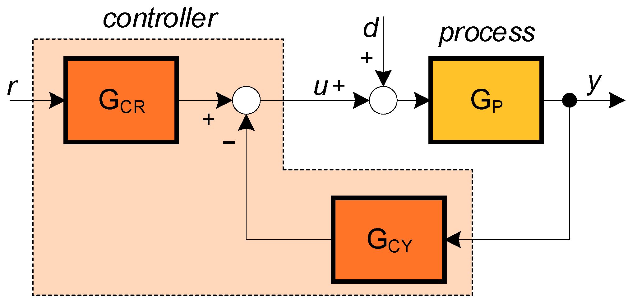
Table 1.
The PIDb controller parameters.
| b | KP | KI | KD |
|---|---|---|---|
| 0 | 0.93011 | 0.23327 | 0.85427 |
| 0.2 | 0.93383 | 0.2486 | 0.85466 |
| 0.5 | 0.85191 | 0.19158 | 0.84114 |
| 0.7 | 0.75396 | 0.11619 | 0.8251 |
| 0.9 | 0.64303 | 0.03635 | 0.80683 |
Table 2.
The calculated characteristic areas for the process models with the additional filter time constant TF = 0.01 s.
Table 2.
The calculated characteristic areas for the process models with the additional filter time constant TF = 0.01 s.
| A0 | A1 | A2 | A3 | A4 | |
|---|---|---|---|---|---|
| GP1 | 1 | 1.41 | 1.5141 | 1.5365 | 1.541 |
| GP2 | 1 | 1.01 | 0.5101 | 0.17177 | 0.04338 |
| GP3 | 1 | 4.01 | 10.0401 | 20.1004 | 35.201 |
| GP4 | 1 | 4.01 | 7.0401 | 10.0704 | 13.1007 |
Table 3.
The calculated PIDb controller parameters.
| b = 0 | b = 0.5 | b = 0.7 | |||||||
|---|---|---|---|---|---|---|---|---|---|
| KP | KI | KD | KP | KI | KD | KP | KI | KD | |
| GP1 | 2.6269 | 1.3991 | 1.4661 | 2.2778 | 1.1385 | 1.418 | 1.8731 | 0.63473 | 1.365 |
| GP2 | 1.128 | 0.47494 | 0.33942 | 1.0017 | 0.3258 | 0.30958 | 0.89095 | 0.18652 | 0.28414 |
| GP3 | 0.37914 | 0.04554 | 0.57814 | 0.3454 | 0.03499 | 0.55729 | 0.30728 | 0.02075 | 0.53411 |
| GP4 | 0.33133 | 0.03935 | 0.39492 | 0.2785 | 0.02479 | 0.34757 | 0.24024 | 0.01344 | 0.31634 |
Table 4.
The calculated characteristic areas for the process models.
| A0 | A1 | A2 | |
|---|---|---|---|
| GP1 | 1 | 4.5 | 18.125 |
| GP2 | 1 | 4.5 | 14.125 |
| GP3 | 1 | 4.5 | 12.125 |
| GP4 | 1 | 4.5 | 10.25 |
Table 5.
The calculated PI controller parameters.
| b = 0 | b = 0.5 | |||
|---|---|---|---|---|
| KI | KP | KI | KP | |
| GP1 | 0.0065 | 0.1142 | 0.0048 | 0.1134 |
| GP2 | 0.0073 | 0.1211 | 0.0052 | 0.1182 |
| GP3 | 0.0078 | 0.1253 | 0.0055 | 0.121 |
| GP4 | 0.0084 | 0.1298 | 0.0058 | 0.1239 |
Table 6.
The calculated characteristic areas for the process models with the additional filter time constant TF = 0.01 s.
Table 6.
The calculated characteristic areas for the process models with the additional filter time constant TF = 0.01 s.
| A0 | A1 | A2 | A3 | A4 | |
|---|---|---|---|---|---|
| GP1 | 1 | 4.51 | 18.170 | 72.703 | 290.813 |
| GP2 | 1 | 4.51 | 14.170 | 38.663 | 97.973 |
| GP3 | 1 | 4.51 | 12.170 | 25.643 | 46.592 |
| GP4 | 1 | 4.51 | 10.295 | 15.895 | 18.721 |
Table 7.
The calculated PIDb controller parameters.
| b = 0 | b = 0.5 | |||||
|---|---|---|---|---|---|---|
| KP | KI | KD | KP | KI | KD | |
| GP1 | 4.4939 | 1.7606 | 4.7353 | 3.4387 | 1.3668 | 4.4883 |
| GP2 | 0.44499 | 0.054126 | 0.82917 | 0.40688 | 0.044121 | 0.81421 |
| GP3 | 0.31757 | 0.033077 | 0.52446 | 0.28765 | 0.024817 | 0.50058 |
| GP4 | 0.25619 | 0.024309 | 0.34998 | 0.22777 | 0.01677 | 0.32033 |
Table 8.
The intermediate calculated parameters for the reference filters calculations.
| Process | KP1 | KD1 | KM | b1m | Tdm | a1m | a2m | KCL |
|---|---|---|---|---|---|---|---|---|
| GP1 | 1.2651 | 1.2838 | 1 | 0 | 0.2 | 1.2 | 0.2 | 3 |
| GP2 | 0.74265 | 0.25007 | 1 | 0 | 1 | 0.0101 | 0 | 3 |
| GP3 | 0.249005 | 0.498512 | 1 | 0 | 0.935822 | 3.06418 | 2.69459 | 3 |
| GP4 | 0.193831 | 0.277263 | 1 | −1.99879 | 0.011 | 1.99021 | 0.982906 | 3 |
Table 9.
The PIDf2 controller reference filter parameters.
| Process | bF2 | bF1 |
|---|---|---|
| GP1 | 0.59091 | 1.0871 |
| GP2 | 0.52881 | 1.0284 |
| GP3 | 9.2833 | 4.3089 |
| GP4 | 5.3174 | 3.2611 |
Table 10.
The PIDfh controller reference filter parameters.
| Process | bF5 | bF4 | bF3 | bF2 | bF1 | Tdm | TCL | n |
|---|---|---|---|---|---|---|---|---|
| GP1 | 0.019465 | 0.24389 | 0.83779 | 1.5782 | 1.7776 | 0.2 | 0.26348 | 2 |
| GP2 | 0.0036331 | 0.25639 | 0.93567 | 1.716 | 1.8749 | 1 | 0.44884 | 2 |
| GP3 | 33.5171 | 93.952 | 72.4423 | 30.8295 | 7.85696 | 0.935822 | 1.33866 | 2 |
| GP4 | 0.390273 | 25.8753 | 30.9495 | 18.5847 | 6.41596 | 0.011 | 1.71971 | 2 |
© 2020 by the authors. Licensee MDPI, Basel, Switzerland. This article is an open access article distributed under the terms and conditions of the Creative Commons Attribution (CC BY) license (http://creativecommons.org/licenses/by/4.0/).
Share and Cite
MDPI and ACS Style
Kos, T.; Huba, M.; Vrančić, D. Parametric and Nonparametric PID Controller Tuning Method for Integrating Processes Based on Magnitude Optimum. Appl. Sci. 2020, 10, 6012. https://0-doi-org.brum.beds.ac.uk/10.3390/app10176012
AMA Style
Kos T, Huba M, Vrančić D. Parametric and Nonparametric PID Controller Tuning Method for Integrating Processes Based on Magnitude Optimum. Applied Sciences. 2020; 10(17):6012. https://0-doi-org.brum.beds.ac.uk/10.3390/app10176012
Chicago/Turabian StyleKos, Tomaž, Mikuláš Huba, and Damir Vrančić. 2020. "Parametric and Nonparametric PID Controller Tuning Method for Integrating Processes Based on Magnitude Optimum" Applied Sciences 10, no. 17: 6012. https://0-doi-org.brum.beds.ac.uk/10.3390/app10176012
Note that from the first issue of 2016, this journal uses article numbers instead of page numbers. See further details here.