Predictive Scheduling with Markov Chains and ARIMA Models

Abstract

Production scheduling is attracting considerable scientific interest. Effective scheduling of production jobs is a critical element of smooth organization of the work in an enterprise and, therefore, a key issue in production. The investigations focus on improving job scheduling effectiveness and methodology. Due to simplifying assumptions, most of the current solutions are not fit for industrial applications. Disruptions are inherent elements of the production process and yet, for reasons of simplicity, they tend to be rarely considered in the current scheduling models. This work presents the framework of a predictive job scheduling technique for application in the job-shop environment under the machine failure constraint. The prediction methods implemented in our work examine the nature of the machine failure uncertainty factor. The first section of this paper presents robust scheduling of production processes and reviews current solutions in the field of technological machine failure analysis. Next, elements of the Markov processes theory and ARIMA (auto-regressive integrated moving average) models are introduced to describe the parameters of machine failures. The effectiveness of our solutions is verified against real production data. The data derived from the strategic machine failure prediction model, employed at the preliminary stage, serve to develop the robust schedules using selected dispatching rules. The key stage of the verification process concerns the simulation testing that allows us to assess the execution of the production schedules obtained from the proposed model.

1. Introduction

While conducting their activities, manufacturing enterprises establish a range of various goals. Certainly, one of the common strategic business objectives is to strengthen the market position. An enterprise that aims to broaden the group of clients, as well as foster the already existing business relations, must first and foremost be reliable and deliver quality goods within contractual deadlines [1,2]. Therefore, proper planning of works becomes central to sound execution of production processes. Production scheduling is the solution that can boost the capacity of manufacturers, hence there are numerous scientific publications in the field [3]. Researchers are still taking active efforts to optimise the effectiveness of production jobs scheduling in order to streamline the production planning process [2,4].

Unfortunately, most of the proposed solutions display numerous limitations [5]. It is common practice that the job scheduling algorithms build schedules for idealized production environments, i.e., assuming a static and stable production flow [5,6]. Thereby, a number of disruptive factors are excluded, which would bring the production to a halt in case they occur [7,8]. As a consequence, contractual deadlines would be missed, penalties would be imposed and the manufacturer’s credibility would diminish. Among the various uncertainty factors, we can highlight the following [5,9]:

• disruptions of resource availability (machine or robot failure)
• disruptions of orders (placement of new orders)
• disruptions of processes (material shortage, poor product quality)
• disruptions associated with misestimation of the ongoing process parameters (incorrect estimation of operation times)
• disruptions related to the change in the duration of the operation (employee absence or malaise, shorter or extended operation times)

Scheduling production in real manufacturing systems cannot afford to pretend to be disruption-free. It is, therefore, of the essence that scheduling endeavors should consider production problems under uncertainty, which is capable of having a colossal effect on the timeliness of production [10,11]. Given that the more the process changes, the greater its disorganization, the scientific literature in the field of scheduling has recently turned towards robust scheduling [5,9].

The predictive scheduling method proposed in this work employs Markov chains and ARIMA (auto-regressive integrated moving average) models whose combination enables determining the values of the machine failure parameters (time to failure and repair time of the machine). In the next step time buffers are directly integrated into the scheduling process and determine the completion time of the production, which corresponds to the delivery date agreed with the customer.

Section 2 summarizes the essential information regarding robust production scheduling and reviews existing literature. The new methodology for scheduling under machine failure and failure prediction is described in Section 3, and the proposed solutions and results are discussed in the subsequent section. Conclusions and plans for further research work are presented in the last section of the work.

2. Existing Work on Robust Production Scheduling

2.1. Essentials of Robust Scheduling

The purpose of a robust production schedule is predominantly to absorb potential disruptions, by allowing variability to the production system parameters.

Two phases of scheduling are distinguished [9,12]:

• Predictive scheduling-related to the planning stage.
• Reactive scheduling-related to the production stage.

A well-executed process of scheduling production jobs must pertain to the first of the phases (also referred to as the offline phase) when the available production data give the foundation for creating [3]:

• a nominal schedule-based on the current system parameters,
• a robust schedule-based on the assumption of uncertainty and variability of production.

Reasonable scheduling in this phase requires not only implementing appropriate tools but also suitable methods for determining uncertainty factors [6]. Unfortunately, there is a distinct paucity of solutions that consider the impact of process disruptions [5,6].

2.2. Existing Literature on Robust Production Scheduling

Due to the practical nature of the problem, robust production scheduling solutions are mainly developed for flow-shop and job-shop systems, which are the prevailing forms of organization in real production systems.

Although robust task scheduling in a flow-shop environment is rather neglected in the literature, a certain number of publications on this issue can be found [13,14,15]. Various approaches have been applied to building robust schedules in a flow-shop environment—from classical local search algorithms [16] to genetic algorithms [17], integer programming applications [18] and dynamic programming [19]. However, in an overwhelming majority, the publications are concerned with predictive-reactive scheduling, thus, tend to focus on the investigation of effective re-scheduling methods [19], and not on the analysis of uncertainty factors itself.

The second most-investigated scheduling problem is robust production scheduling in job-shop systems [20]. This system is a close reflection of a typical production environment, where the order of operations is imposed by the technological routes of their jobs. Researchers have long highlighted that the real job-shop problem requires a distinctly different approach than the shown by the prevailing theoretical tendencies [21], however, to date no clear trend has emerged. Robust scheduling solutions proposed in the aspects of job-shop production processes resemble the solutions for flow-shop systems inasmuch as they are mainly dedicated to the predictive-reactive approach. Standard approaches are shown to draw from various methods, such as genetic algorithms and their hybrids [20,22], immunological algorithms [23,24] and stochastic programming [25]. Other authors propose robust scheduling methods using expert systems [26].

2.3. Machine Failure as the Major Uncertainty Factor

Although many uncertainty factors can be named, the failure of technological machinery is still considered to be the central problem in manufacturing. This disturbance is regarded to have the greatest impact on performed processes. Failure will not only halt the production but its consequences will linger throughout the remaining production process [5,7].

From the analyzed scientific papers dealing with the topic of machine failure in scheduling, it can be seen that the search for methods that will enable approaching the problem of machine failure and predicting its occurrence are very much in place. Developing effective prediction methods is extremely important from the perspective of robust scheduling [18,19,26].

To this end, a probability distribution is among the most widely used approaches in the field of failure analysis. Researchers employ typical distributions and their combinations. The failure description proposed by Jensen [27] applies a uniform distribution. A similar solution is proposed by Al-Hinai and ElMekkawy [28], who, however, assume that the probability of failure is constant. In contrast, in their description of production process disturbances, Davenport et al. [29] implement a normal distribution, while Mehta and Uzsoy [21] utilize an exponential distribution. The authors propose the use of interesting approaches, such as the methods based on combinations of various distributions. The latter is used by Gürel et al. [4], who combine normal, triangular and exponential distributions.

Recently, researchers have also investigated the application of typical key performance indicators (KPIs) used in maintenance, e.g., MTTF (mean time to failure), MTBF (mean time between failures) and MTTR (mean time to repair). In their direct application of the indicators, Deepu [9] and Gao [5] analyze specially prepared scenarios that assume a certain frequency of machine failure, i.e., high, medium or low, to study the consequences of machine downtime and propose solutions to absorb the emerging disruptions to the schedule. With respect to the indirect use of the indicators, Kempa et al. [30,31] propose the use of the aforementioned reliability indicators indirectly for the purpose of estimating Weibull distribution parameters, while Rosmaini and Shahrul [32] in their study, couple the said indicators with statistical methods. These studies, however, suffer from the major drawback—the acquisition and use of the respective quantities is treated quite theoretically and lacks practical verification on real data of machine failure rates [9,31].

In addition to the methods referenced in the preceding paragraphs, a range of alternative failure prediction methods can be found in the literature. Jian et al. [20] propose accumulating failures to a single occurrence, describing it by means of the MTTR parameter and their original indicator, MBL (machine breakdown level). In turn, Rawat and Lad [33] determine failure rates from the analysis of machine load time distributions, and Baptista et al. in [34] use artificial neural networks for failure analysis.

Although constituting an interesting and important voice in the robust production scheduling studies, these models are associated with certain limitations. Their verification is often carried out on test data, which may not be the most accurate representation of actual problems in manufacturing systems. Secondly, the questions arise as to insufficient argumentation regarding the selection of the solutions. Consequently, the key aspect of implementing historical data in studies of the failure rate of machines is omitted.

The need to use real data on uncertainty factors is also emphasized by Davenport et al. [29] and Kalinowski et al. [35]. Only real knowledge on process disruptions can actually solve actual the problems that result from their occurrence. The issue was addressed in our previous work [36], where a model for the prediction of technological operation times in the framework of an intelligent job scheduling system was conceptualized. The study in question considered the impact of real processing time uncertainty on the production schedule and the developed intelligent module also implemented ARMA/ARIMA time series models, however, a problem of a different size was concerned and the verification was carried out for different production data. While such solutions can be found in the literature, the body of knowledge in the field still appears to lack proper depth [6].

3. Production Scheduling under Technological Machine Failure Constraint

3.1. Objectives

This paper formulates a predictive production scheduling process model in the job-shop environment under technological machine failure established with the help of Markov chains and ARIMA models. Our solutions predict the time of machine failure, as well as the time of repair, and constitute an alternative method to the models proposed in the literature. The objective function of our predictive production scheduling is to minimize the makespan, i.e., to produce a schedule with a minimum completion time of all jobs.

3.2. Basic Mathematical Notation of the Problem

Prior to formulating the problem of robust job scheduling under uncertainty in the job-shop system, we need to define the elements of the production process:

• Set $M$ is a set of $m$ machines (workstations) processing jobs:

  $$M=\left\{M_1,M_2,\dots ,M_m\right\}.$$

  (1)
• Set $J$ is a set of $n$ jobs (tasks) to process

  $$J=\left\{J_1,J_2,\dots ,J_n\right\}.$$

  (2)

Processing job J_i on machine M_j constitutes an operation, which is called operation j of job i in the following. Therefore, it is necessary to define:

• $MO$—a matrix of $m$ columns and $n$ rows describing the technology (the job order):

  $$MO=\left[o_{ij}\right],$$

  (3)

  where $o_{ij}$—the order position of the operation $j$ of job $i$, which is $o_{ij}=0$ when the job is not processed on the machine; and $o_{ij}=\left\{1,\dots ,m\right\}$, when it is.
• Matrix $PT$—a matrix describing processing times of operations:

  $$PT=\left[p{t}_{ij}\right],$$

  (4)

  where $p{t}_{ij}$—the processing time of operations $j$ of job $i$; for each $o_{ij}=0$, $p{t}_{ij}=0$.
• Set $F{T}_{Ml}$ of potential machine failure times:

  $$F{T}_{Ml}=\left\{f{t}_{M{l}_1},f{t}_{M{l}_2},\dots ,f{t}_{M{l}_z}\right\},l\in \langle 1;m\rangle ,$$

  (5)

  where $f{t}_{M{l}_z}$—time to failure of the machine l; where $z$ is a natural number representing the z-th machine failure.
• Set $T{B}_{Ml}$ of time buffers to include in the nominal schedule (for machine $l$) to obtain a robust schedule:

  $$T{B}_{Ml}=\left\{t{b}_{M{l}_1},t{b}_{M{l}_2},\dots ,t{b}_{M{l}_z}\right\},$$

  (6)

  where $t{b}_{M{l}_z}$—the size of the time buffer in the schedule at the failure time $f{t}_{M{l}_z}$; where for $f{t}_{M{l}_z}\ne 0$, $t{b}_{M{l}_z}\ne 0$.

3.3. Prediction of Failure and Machine Repair Times

In the paper, we analyze the system describing the shift on which a failure occurs. Additionally, the repair time [37] required for failure removal is analyzed. Let $\left(\mathsf{\Omega },ℱ,P\right)$ be a probabilistic space: $\mathsf{\Omega }$—sample space (set of elementary events, outcomes), field $ℱ$ is a family of sample space $\mathsf{\Omega }$ (set of all subsets of sample space $\mathsf{\Omega }$), $P$—probability measure (function that assigns each element from field $ℱ$ the probability, the value between 0 and 1), $N$—a set of natural numbers,$R$—a set of real numbers, $S=\left\{s_1,s_2,\dots ,s_k\right\}$—a set of possible shifts, $k\in N$, $k<\infty$—the number of possible shifts.

Definition 1.

A family${\left\{X_t\right\}}_{t\in N}$ of random variables$X_t:\Omega \to S$for any$t\in N$is called a stochastic process with discrete time [38,39].

At any $t \in N$ time, the system can take one of the possible states denoted as $X_t\left(\omega \right)=x_t\in S$ and $P\left(X_t\left(\omega \right)=s_i\right)=p_i\left(t\right)$ value means the probability that the system is in a state $s_i\in S$,$1\le i\le k$ at a moment $t\in N$, and ${\displaystyle \sum }_{i=1}^k{p}_i\left(t\right)=1$.

Definition 2.

A stochastic process${\left\{X_t\right\}}_{t\in N}$with a discrete time is called a Markov chain [38,39]. If for each $n\in N$ , moments $t_1,t_2,\dots ,t_n\in N$ satisfying the condition  $t_1<t_2<\dots <t_n$ and any  $x_1, x_2,\dots , x_n \in S,$ the equality:

$$P\left(X_{t_n}=x_n|X_{t_{n-1}}=x_{n-1}, X_{t_{n-2}}=x_{n-2}, \dots , X_{t_1}=x_1\right)=P\left(X_{t_n}=x_n|X_{t_{n-1}}=x_{n-1}\right),$$

(7)

holds.

Below we assume $t_n=n\in N$. If ${\left\{X_t\right\}}_{t\in N}$ is a heterogeneous Markov chain, then for any $t\in N$ and $1\le i,j\le k$, the value:

$$P\left(X_t=s_j|X_{t-1}=s_i\right)=p_{ij}\left(t\right),$$

(8)

is the transition probability from $s_i$ state at the moment $t-1$ to $s_j$ state at moment $t$. From Markov property (7), the conditional probability distribution of the future process state depends only on the current state at moment $t$, regardless of the past. The matrix $P\left(t\right)={\left[p_{ij}\left(t\right)\right]}_{1\le i,j\le k}$ is called the transition probabilities matrix at the moment $t$ and the elements of the $P\left(t\right)$ matrix satisfy the condition ${\displaystyle \sum }_{j=1}^k{p}_{ij}\left(t\right)=1$ for $t\in N$ and $1\le i\le k$.

Definition 3.

The Markov chain  ${\left\{X_t\right\}}_{t\in N}$ is homogeneous, if the probabilities of transition  $p_{ij}\left(t\right)$ do not depend on the moment $t\in N$.

Thus, if for a homogeneous Markov chain [39,40] the matrix $P={\left[p_{ij}\right]}_{1\le i,j\le k}$ satisfies the condition ${\displaystyle \sum }_{j=1}^k{p}_{ij}=1$, $1\le i\le k$, then it is known as the one-step transition probability matrix. From the above, for a homogeneous Markov chain, the transition probability from $s_i$ state at $t$ moment to the $s_j$ state at $t+n$ moment is calculated as follows [38,40]:

$$P\left(X_{t+n}=s_j|X_t=s_i\right)=p_{ij}{}^{\left(n\right)}$$

(9)

where ${\left[p_{ij}^{\left(n\right)}\right]}_{1\le i,j\le k}=P^n$, $n\in N$ is the transition probability matrix in $n$ steps.

Definition 4.

If${\left\{X_t\right\}}_{t\in N}$ is a homogeneous Markov chain and there is a distribution  $\pi =\left({\pi }_1,{\pi }_2,\dots ,{\pi }_k\right)$ where  ${\pi }_i\ge 0$, $1\le i\le k$ and  ${\displaystyle \sum }_{i=1}^k{\pi }_i=1$ satisfying the equation:

$$\pi P=\pi$$

(10)

then the distribution $\pi$ is called the stationary distribution of the homogeneous Markov chain.

This property means that if at some $n\in N$ moment the chain reaches a stationary distribution, then for each subsequent moment greater than $n$, the distribution will remain the same. To determine the stationary distribution, we solve Equation (10).

Let ${\left\{x_t\right\}}_{0\le t\le n}$ be the realization of Markov chain, where $n_i=\#\left\{t:x_t=s_i,0\le t\le n\right\}$ is the number of moments for which the system was in $s_i$ state, $1\le i\le k$ and ${\displaystyle \sum }_{i=1}^k{n}_i=n$. The value $n_{ij}=\#\left\{t:x_t=s_i,x_{t+1}=s_j,0\le t\le n-1\right\}$ represents the number of transitions from the state $s_i$ to the state $s_j$ for $1\le i,j\le k$ and ${\displaystyle \sum }_{j=1}^k{n}_{ij}=n_i$. We calculate the estimator of transition probability from $s_i$ state to $s_j$ state as ${\widehat{p}}_{ij}=\frac{n_{ij}}{n_i}$ for $1\le i,j\le k$.

In this work, the goodness of fit test is used to verify Markov property ${\chi }^2$ [40,41]. At the significance level $\alpha \in \left(0,1\right)$, we create a working hypothesis: $H_0:P\left(X_t=x|X_{t-1}=y,X_{t-2}=z\right)=P\left(X_t=x|X_{t-1}=y\right)$ (the chain ${\left\{X_t\right\}}_{t\in N}$ meets Markov property) and an alternative hypothesis: $H_1:P\left(X_t=x|X_{t-1}=y,X_{t-2}=z\right)\ne P\left(X_t=x|X_{t-1}=y\right)$ (the chain ${\left\{X_t\right\}}_{t\in N}$ does not meet Markov property), where $x,y,z\in S$.

To verify the hypothesis $H_0$, we calculate the test statistics:

$${\chi }_e^2={{\displaystyle \sum }}_{i=1}^k{{\displaystyle \sum }}_{j=1}^k{{\displaystyle \sum }}_{v=1}^k\frac{{\left(n_{ijv}-n_{ij}{\widehat{p}}_{jv}\right)}^2}{n_{ij}{\widehat{p}}_{jv}},$$

(11)

which has a ${\chi }^2$ distribution with $k^3$ degrees of freedom and $n_{ijv}=\#\left\{t:x_t=s_i,x_{t+1}=s_j,x_{t+2}=s_v, 0\le t\le n-2\right\}$ is the number of transitions from state $s_i$ to state $s_j$ and next to state $s_v$ for $1\le i,j,v\le k$. The critical value is a quantile of order $1-\alpha$ for ${\chi }^2$ distribution with $k^3$ degrees of freedom. We denote as ${\chi }^2\left(1-\alpha ,k^3\right)$. If ${\chi }_e^2<{\chi }^2\left(1-\alpha ,k^3\right)$, then at the significance level $\alpha$, there are no grounds for rejecting the working hypothesis $H_0$. So, we can assume that the chain ${\left\{X_t\right\}}_{t\in N}$ meets Markov property. When ${\chi }_e^2\ge {\chi }^2\left(1-\alpha ,k^3\right)$, then at the significance level $\alpha$ we reject the working hypothesis $H_0$ in favor of the alternative hypothesis. Thus, the chain ${\left\{X_t\right\}}_{t\in N}$ does not meet Markov property.

An ARIMA model, which usually correlates historical values in a time series, is applied to forecast the repair time. The behavior of the considered time series can be predicted (i.e., forecast with appropriate probability) based on current observation and historical data (dataset). Let ${\left\{r{t}_t\right\}}_{t\in N}$ denote the sequence of times needed to repair a plant. Because the times needed do remove the failures can take only positive values, the variance-stabilizing transformation

$${\epsilon }_t=ln\left(r{t}_t\right)$$

(12)

can be applied.

The series ${\left\{{\epsilon }_t\right\}}_{t\in N}$ is identified using $ARIMA\left(p,r,q\right)$ models, $p,r,q\in N$ (auto-regressive integrated moving average) [42,43,44,45]. In this paper, the logarithm of repair time is modelled as follows:

$${\Delta }^r{\epsilon }_t={\alpha }_0+{\alpha }_1{\Delta }^r{\epsilon }_{t-1}+\dots +{\alpha }_p{\Delta }^r{\epsilon }_{t-p}+{ϵ}_t-{\theta }_1{ϵ}_{t-1}-\dots -{\theta }_q{ϵ}_{t-q}$$

(13)

where ${\left\{{ϵ}_t\right\}}_{t\in N}$ is a sequence of independent random variables with distribution $N\left(0, {\sigma }^2\right)$. To estimate the integration degree, Augmented Dickey-Fuller (ADF) and the Kwiatkowski-Phillips-Schmidt-Shin (KPSS) [42,46,47] tests are applied.

The Markov chains and ARIMA models are implemented to determine the values of elements of sets $F{T}_{Ml}$ and $T{B}_{Ml}$. The analysis of historical machine failure data leads to determining important failure parameters, which can subsequently help establish buffer time periods in the predictive production scheduling method.

4. Experimental Verification of the Proposed Solution

4.1. Historical Data

In order to verify the solutions proposed in this publication, a process of robust job scheduling is performed on the production data and on historical data of technological machine failure. The production data describes the execution of 9 production jobs processed by 12 machines, constituting a manufacturing cell (

Table 1. Production data implemented in the robust scheduling solution.

Job	Operation		Machine	Type of Operation	tsij * [min]	tsij * [h]	toij * [min]	toij * [h]
2	10	M1	Laser1	Laser-cutting sheets	22	0.367	4	0.067
	20	M4	CNC saw	Band-saw cutting	6	0.100	0.5	0.008
	30	M3	CNC press	Edge bending	16	0.267	3	0.050
	40	M8	Drill	Drilling holes and threading	12	0.200	1	0.017
	50	M5	Metalworking	Metalworking	5	0.083	1	0.017
	60	M6	MIG welder	MIG welding	8	0.133	5.5	0.092
6	10	M1	Laser1	Laser-cutting sheets	12	0.200	0.3	0.005
	20	M2	Laser2	Laser-cutting profiles	14	0.233	1	0.017
	30	M5	Metalworking	Metalworking	5	0.083	1	0.017
	40	M6	MIG welder	MIG welding	8	0.133	1	0.017
	50	M10	Turning lathe	Turning	11	0.183	2	0.033
9	10	M1	Laser1	Laser-cutting sheets	20	0.333	5	0.083
	20	M2	Laser2	Laser-cutting pipes and profiles	12	0.200	2	0.033
	30	M4	CNC saw	Band-saw cutting	6	0.100	1	0.017
	40	M3	CNC press	Edge bending	25	0.471	6.5	0.108
	50	M8	Drill	Drilling holes and threading	12	0.200	7	0.117
	60	M5	Metalworking	Metalworking	5	0.083	2	0.033
	70	M6	MIG welder	MIG welding	8	0.133	7.5	0.125

* ts_ij—setup time, to_ij—operation time.

). The parts are produced in batches of 50 elements ($b=50)$ and the setup times of individual operations are not taken into account in the production scheduling process (uncertainty of setup times is a different factor and requires additional research). Therefore:

$$p{t}_{ij}=b ·t{o}_{ij},$$

(14)

where $b$—quantity of elements in the production batch, $t{o}_{ij}$—operation time.

The data describing the failure rate of machines in the scheduled production process have been obtained from the computer records of machine operation from a maintenance department (

Table 2. Machine failure and repair time data implemented in the scheduling solution.

Machine M1		Machine M2		Machine M3		Machine M6		Machine M7		Machine M8
Failure–Shift [–]	Repair Time [min]	Failure –Shift [–]	Repair Time [min]	Failure–Shift [–]	Repair Time [min]	Failure–Shift [–]	Repair Time [min]	Failure–Shift [–]	Repair Time [min]	Failure–Shift [–]	Repair Time [min]
3	230	2	50	3	70	1	10	2	20	2	235
2	120	1	15	3	30	1	50	1	20	1	30
1	15	2	20	1	35	1	15	1	40	1	15
2	95	2	20	3	190	3	110	1	20	2	215
1	80	1	15	2	125	1	120	2	20	2	100
2	30	3	250	2	30	2	130	3	80	2	10
3	130	2	15	3	15	1	30	2	10	1	40

). The collected data describe the failure rate of six technological machines that are crucial for the performed production process. The numbers of observations are as follows:

• Machine M₁—197 observations
• Machine M₂—166 observations
• Machine M₃—180 observations
• Machine M₆—157 observations
• Machine M₇—208 observations
• Machine M₈—97 observations

The nominal and robust schedules are subsequently built based on the data presented above. This, however, must be preceded by the prediction of failure parameters with the application of Markov chain and ARIMA models, which is described in the next section.

4.2. Prediction of Machine Failure Parameters

The failure prediction process is performed using appropriate scripts formulated in the RStudio computing environment [48] that enable the analysis in the range described in Section 3.3.

Modelling the machine failure rates using the Markov chain (containing information on changes in production) is performed with the use of the markovchain library. Initially, the collected empirical data is verified to check whether they fulfil the properties of the Markov process. The analyses confirm that the data from the analyzed machines meet the required properties, which is further evidenced by the p-value index (

Table 3. Markov process identification results.

Machine No.	p-Value [–]
M1	0.8922
M2	0.9051
M3	0.9510
M6	0.7361
M7	0.9684
M8	0.5618

). The p-value is the probability of obtaining hypothesis test results as extreme as the observed results, assuming that the null hypothesis is correct (data chain has a Markov property).

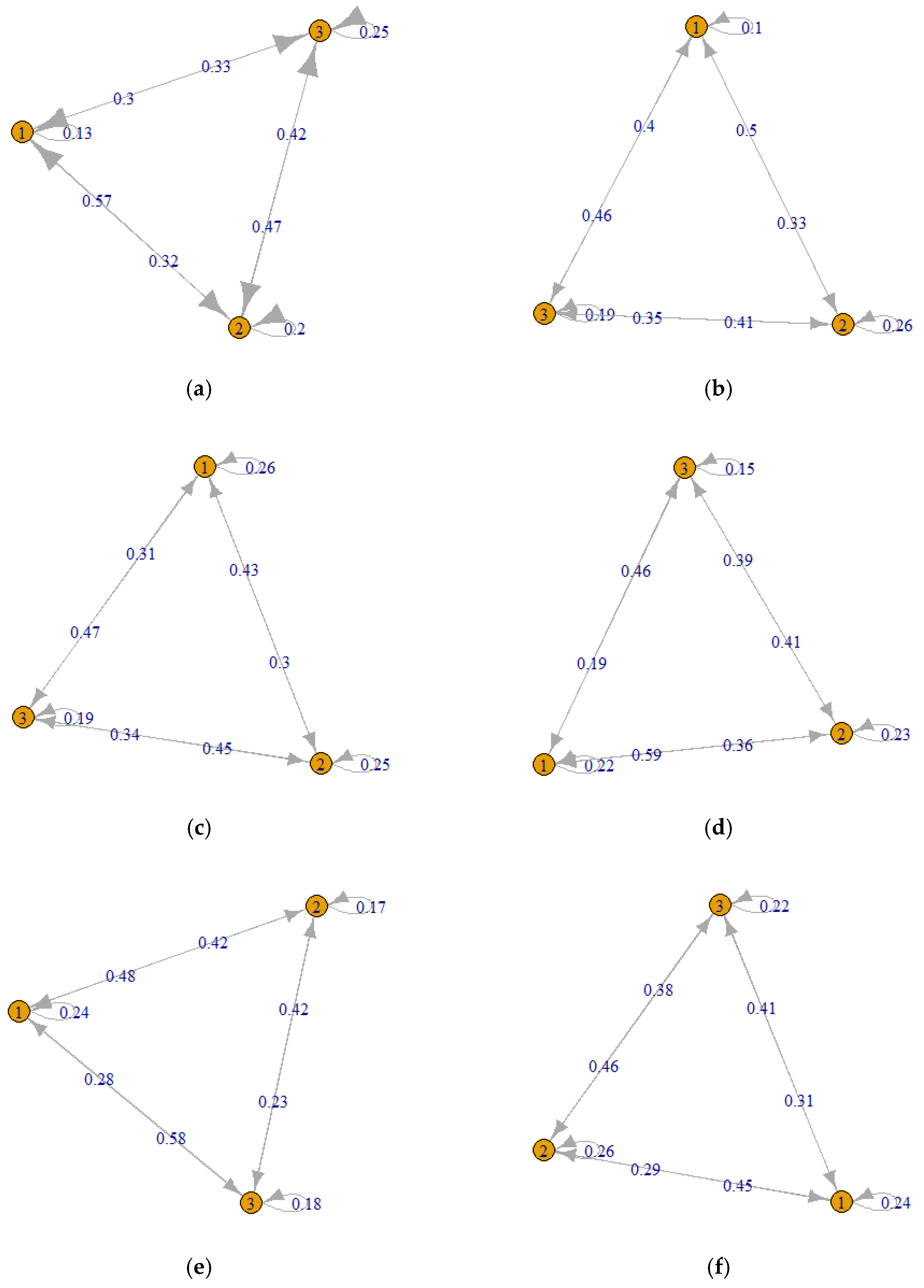
In the next stage of the machine failure prediction analysis, the transition rate matrices are generated from the collected data. From the obtained information, we determine, at a given probability level, the occurrence of subsequent chain elements, which in this study is the probability of machine failure occurrence at subsequent production shifts (

Table A1. The transition rate matrix for each machine in the production system. Bold numbers represent the highest probability of the machine failure.

Transition Rate Matrix
Machine M1				Machine M2				Machine M3
shift	1	2	3	shift	1	2	3	shift	1	2	3
1	0.132	0.566	0.302	1	0.100	0.500	0.400	1	0.262	0.426	0.311
2	0.324	0.203	0.473	2	0.328	0.262	0.410	2	0.300	0.250	0.450
3	0.333	0.420	0.246	3	0.463	0.352	0.185	3	0.466	0.345	0.190
Machine M6				Machine M7				Machine M8
shift	1	2	3	shift	1	2	3	shift	1	2	3
1	0.222	0.593	0.185	1	0.244	0.476	0.280	1	0.241	0.448	0.310
2	0.361	0.230	0.410	2	0.415	0.169	0.415	2	0.286	0.257	0.457
3	0.463	0.390	0.146	3	0.583	0.233	0.183	3	0.406	0.375	0.219

).

For clarity of presentation, the results from calculations are given in the form of transition diagrams (Figure 1), which additionally enable determining the probability of failure not only on subsequent shifts but also during the current shift (the arrow returning to the node). In Figure 1, knots represent shifts and the probability of machine failure during a given shift is given at the beginning of each arrow (next to the knot), e.g., for machine M₆, the probability that the machine failure will occur after shift 1 during shift 2 is 0.593.

The second key parameter of failure is its time. To this end, the forecast package is used, which enables identifying the elements of ARIMA time series. As a result, the predicted machine failure repair times are determined. Before forecasting, each machine is tested to verify whether the process is stationary, also the component models are established (autoregression, moving average and the integration). In the subsequent step, future repair times are predicted. Due to the fact that in ARIMA models, the forecasts may also take negative values, the collected observations have been first subjected to variance-stabilizing transformation, and after the prediction, the process is completed and their original sets of values are returned. The results from the model identifying exemplary predicted times for the 5 subsequent steps of the time series are presented in

Table 4. Predicted machine repair times.

Machine No.	ARIMA Model	Predicted Repair Times [min]
		1	2	3	4	5
M1	ARIMA(1,0,0)	38.77	42.11	41.90	41.91	41.91
M2	ARIMA(0,0,0)	39.79	39.79	39.79	39.79	39.79
M3	ARIMA(1,1,2)	36.78	40.80	40.02	40.16	40.14
M6	ARIMA(2,0,1)	48.12	37.57	43.20	37.78	42.13
M7	ARIMA(1,0,1)	54.80	54.20	53.72	53.35	53.06
M8	ARIMA(0,0,1)	51.83	49.85	49.85	49.85	49.85

.

The data below display the disparity between individual machine repair times. Each machine is coupled with a different ARIMA model. From the set of possible ARIMA models, we select a model that has a smaller AIC (Akaike Information Criterion) value. The analytical process is carried out with the exclusive use of autoregression (Machine M₁), or the moving average (Machine M₈), or a combination thereof (Machine M₂, M₆, M₇). In a single case (Machine M₂), time variability is a series of independent random variables; therefore, the forecast repair times are established on the basis of mean observations.

The results of the prediction of machine failure parameters are perfectly applicable to robust production scheduling. Expressing the time of failure through production shifts allows us to determine the intervals in which machine failures are likely to occur. In turn, the forecasted repair times could be further employed to the determination of machine inspection and maintenance times. Therefore, in the next stage, the obtained analysis results are used to formulate a robust production schedule, whose effectiveness is subsequently verified.

4.3. Production Process Modelling and Scheduling

Before the obtained prediction results could be subjected to further processing, nominal schedules are generated from the real data. Let us assume that the product is manufactured in batches of 50 pieces and the objective function of the schedule is to minimize the makespan ($C_{\max }$).

The schedules are developed using LiSA (A Library of Scheduling Algorithms) software [49], for the analysis of scheduling problems in various environments. The production data serve to represent the production system: a set of machines $M$ and jobs $J$, the technology matrix $MO$ and the matrix of processing times $PT$. To test the alternative versions of scheduling, the choice of the next operation is determined by two dispatching rules [50]:

• LPT (longest processing time)
• SPT (shortest processing time)

The robustness of the production schedules is to be provided by the inclusion of the results from the predictions of failure parameters using the data describing the states of production shifts set $S$ and predicted repair times $r{t}_t$. As a result, we have managed to determine the elements from the set of predicted machine failure times $F{T}_{Ml}$ and the service time buffer set $T{B}_{Ml}$. As noted in the introduction, the data obtained for strategic machines are analyzed from the perspective of executed production processes, hence the discrepancies in the designations in the technology records and the schedule. All the data that serve to generate the robust schedule are presented in

Table 5. The data implemented into the robust production schedule.

Machine No.	Elements of Set FTMl [h]	Elements of Set TBMl [h]
M1	FTM1 = {8}	TBM1 = {0.646, 0.702, 0.698, 0.699, 0.699}
M2	FTM2 = {8}	TBM2 = {0.663, 0.663, 0.663, 0.663, 0.663}
M3	FTM3 = {8}	TBM3 = {0.613, 0.680, 0.667, 0.669, 0.669}
M6	FTM6 = {8}	TBM6 = {0.802, 0.626, 0.720, 0.630, 0.702}
M7	FTM7 = {8}	TBM7 = {0.913, 0.903, 0.895, 0.889, 0.884}
M8	FTM8 = {8}	TBM8 = {0.864, 0.831, 0.831, 0.831, 0.831}

.

Since it is built on the data above, the obtained schedule is robust to machine failure disturbances. The procedure for generating the robust schedule is rather straightforward: service time buffers $T{B}_{Ml}$ are implemented into the nominal schedule in the slots indicated by the set of machine failure times $F{T}_{Ml}$. The time-to-failure is counted only for the machines processing jobs (idle time was disregarded). In the case when a service time buffer is required during the operation, any interfering operation was shifted right in the order of jobs.

4.4. Evaluation Criteria

To verify the effectiveness of the robust scheduling solutions, as well as for the sake of comparative analysis against the nominal schedules, the following assessment criteria are applied:

• makespan $C_{\max }$—total production time,
• mean completion time $\overline{C}$ given by:

  $$\overline{C}=\frac{1}{n}{{\displaystyle \sum }}_{i=1}^n\left(C_i\right),$$

  (15)

  where $C_i$—the completion time of job i.
• mean flow time $\overline{F}$ given by:

  $$\overline{F}=\frac{1}{n}{{\displaystyle \sum }}_{i=1}^n\left(F_i\right),$$

  (16)

  where $F_i$—the flow time of job i.
• the number of critical operations $Y_K$ is derived from:

  $$Y_K={{\displaystyle \sum }}_{i=1}^n{{\displaystyle \sum }}_{j=1}^m\left(y_{ij}\right),$$

  (17)

  $$y_{ij}=\{\begin{array}{c}1, when \left(t{z}_{ij}-t{r}_{ij+1})=0\right)\\ 0,when \left(t{z}_{ij}-t{r}_{ij+1})\ne 0\right) \end{array},$$

  (18)

  where $Y_K$—the number of critical operations, $t{z}_{ij}$—the completion time of operation o_ij (current), $t{r}_{ij+1}$—the start time of operation o_ij + 1 (subsequent).

The verification of the obtained schedules is performed during the online stage (production execution), modelled with the Enterprise Dynamics software in a series of simulation tests. The computations serve to determine total completion times of production jobs under strategic machinery failure. The modelling tool used in the study allows detecting machine failure times by setting the MTTF and MTTR indicators and selected probability distributions (

Table 6. Machine failure parameters defined in the simulation environment.

Machine No. (Technology)	MTTF *	MTTR *
M1	Uniform(0, 16.763)	Weibull(0.88, 1.28)
M2	Uniform(0, 8.673)	Weibull(0.75, 1.51)
M3	Uniform(0, 15.247)	Weibull(0.679, 1.72)
M6	Uniform(0, 22.083)	Weibull(0.769, 1.43)
M7	Uniform(0, 8.34)	Weibull(0.973, 1.58)
M8	Uniform(0, 19.24)	Weibull(0.877, 1.45)

* the parameters are expressed in hours.

). The MTTF values are specified for the uniform probability distribution (i.e., the machine failure can occur at any time—from the start of the job on the machine until its completion). On the other hand, the MTTR values are determined using the Weibull distribution, obtained for machine repair times from the Cullen–Frey graph [6].

Twenty-five simulations of the production process are performed for each of the LPT or SPT schedules. The indicators employed in the assessment of the results from simulations are:

• Increase of completion time of all jobs $\Delta C_{\max }$ given by:

  $$\Delta C_{\max }=C_{\max }-{C^{\prime }}_{\max } ,$$

  (19)

  where $\Delta C_{\max }$—increase of completion time of all jobs, $C_{\max }$—nominal schedule makespan, ${C^{\prime }}_{\max }$—actual (executed) schedule makespan.
• Relative increase of makespan $E_{C_{max}}$ given by:

  $$E_{C_{max}}=\frac{C_{\max }}{{C^{\prime }}_{\max }},$$

  (20)

  where $E_{C_{max}}$—relative increase of makespan, $C_{\max }$—nominal schedule makespan, ${C^{\prime }}_{\max }$—actual (executed) schedule makespan.

4.5. Experimental Results

The first of the verification objectives is to compare the nominal and robust production schedules in terms of evaluation criteria. The values of the evaluation indicators of the schedules have been determined and are summarized below (

Table 7. Evaluation criteria in the nominal and robust schedules.

Dispatching Rule	Evaluation Criterion [h]
	$\overline{\mathit{F}}$			$\overline{\mathit{C}}$			${\mathit{C}}_{\mathit{m}\mathit{a}\mathit{x}}$
	Nominal Sched	Robust Sched	Elong. [%]	Nominal Sched	Robust Sched	Elong. [%]	Nominal Sched	Robust Sched	Elong. [%]
LPT	23.34	23.86	2.3%	31.94	36.49	14.2%	46.93	53.14	13.2%
SPT	18.33	19.94	8.8%	20.95	23.42	11.8%	47.26	55.68	17.8%

).

From the presented data, it can be seen that the implementation of service time buffers increases the completion times of all jobs. As a consequence, in each of the analyzed cases, one additional shift is required to complete the production process. This effect is not at all unexpected, given that incorporating service time buffers is inseparably connected with elongation. It should be noted, however, that in the robust schedule the time spent in the production system is not extended owing to the fact that the mean flow time is subject to slight elongation.

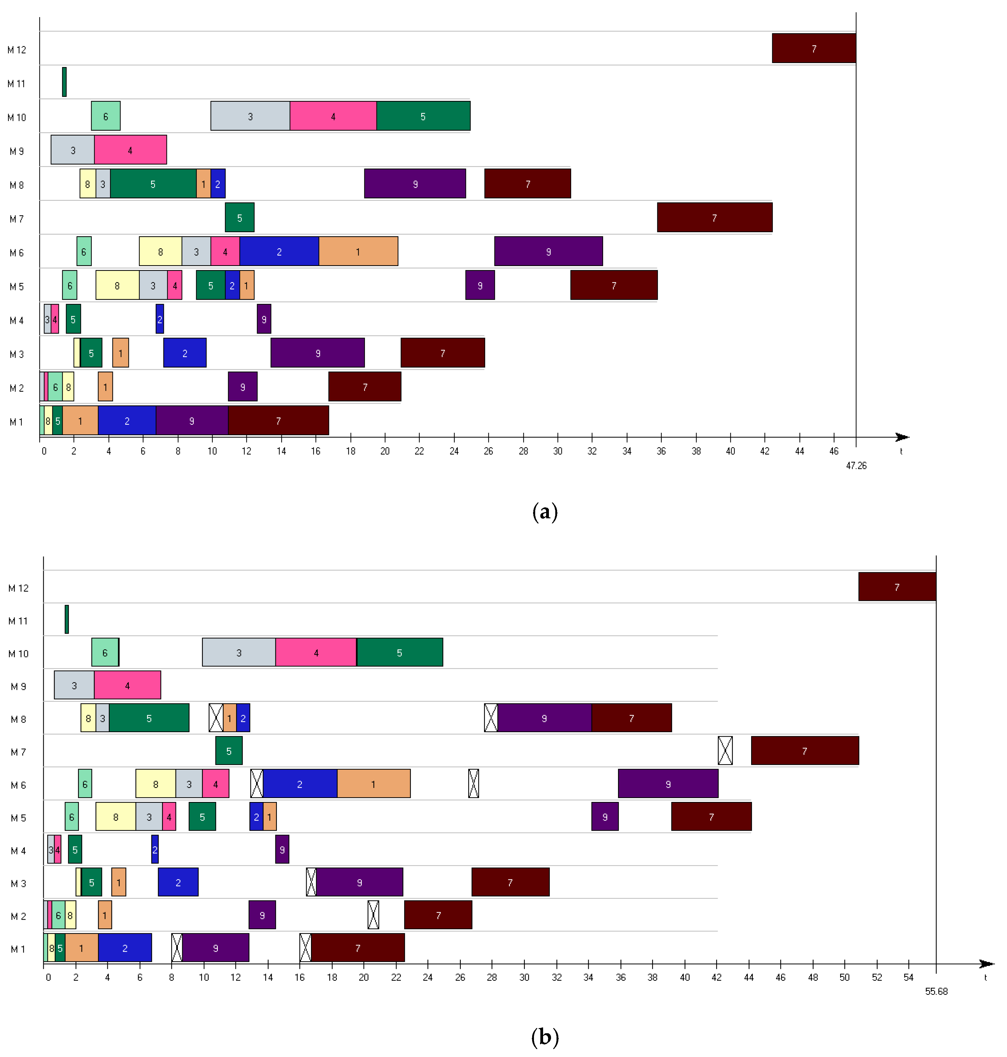
Figure 2 presents the visual interpretation of the nominal and robust SPT schedules. Service time buffers are represented by crossed white blocks.

A further indicator of robustness that is of great importance in scheduling is the number of critical operations. Scheduling should minimize its value because the stability of the executed process is compromised with the rising number of critical operations. In the analyzed example, the number of critical operations is considered in relation to individual jobs ($Y_{KJ}$) and machines ($Y_{KM}$). The robust scheduling results with respect to the number of critical operations are presented in

Table 8. The number of critical operations in the nominal and robust schedules.

Dispatching Rule	Number of Critical Operations [–]
	${\mathit{Y}}_{\mathit{K}\mathit{J}}$			${\mathit{Y}}_{\mathit{K}\mathit{M}}$
	Nominal Sched.	Robust Sched.	Reduction [%]	Nominal Schedule	Robust Sched.	Reduction [%]
LPT	30	24	−20.0%	26	21	−19.2%
SPT	32	27	−15.6%	25	21	−16.0%

.

The incorporation of service time buffers is shown to have a positive effect on the considered parameters. The number of critical operations is reduced by up to 20%. This confirms the legitimacy of implementing service time buffers, which generate additional space in the schedule and thus can prove to be beneficial in the event of machinery failure or other process disruptions.

Simulation tests are conducted to indicate which of the schedules features a makespan closer to the simulated completion time of all jobs. The tests follow the procedure presented in the preceding section and their results are given below, in

Table 9. Results from simulation: nominal and robust schedules (LPT—longest processing time).

Sim. No.	Executed Schedule (Simulation) C′max [h]	Increase of Makespan and Relative Increase of Makespan
		Nominal Schedule			Robust Schedule
		Cmax [h]	ΔCmax [h]	ECmax [–]	Cmax [h]	ΔCmax [h]	ECmax [–]
1	52.15		−5.22	0.90		0.99	1.02
2	49.75		−2.82	0.94		3.39	1.07
3	50.93		−4.00	0.92		2.21	1.04
4	57.57		−10.64	0.82		−4.43	0.92
5	52.79		−5.86	0.89		0.35	1.01
6	52.62		−5.69	0.89		0.52	1.01
7	50.01		−3.08	0.94		3.13	1.06
8	55.23		−8.30	0.85		−2.09	0.96
9	50.69		−3.76	0.93		2.45	1.05
10	53.73		−6.80	0.87		−0.59	0.99
11	50.62		−3.69	0.93		2.52	1.05
12	49.26	46.93	−2.33	0.95	53.14	3.88	1.08
13	51.98		−5.05	0.90		1.16	1.02
14	51.73		−4.80	0.91		1.41	1.03
15	50.20		−3.27	0.93		2.94	1.06
16	52.17		−5.24	0.90		0.97	1.02
17	50.71		−3.78	0.93		2.43	1.05
18	51.01		−4.08	0.92		2.13	1.04
19	50.61		−3.68	0.93		2.53	1.05
20	50.65		−3.72	0.93		2.49	1.05
21	49.95		−3.02	0.94		3.19	1.06
22	50.22		−3.29	0.93		2.92	1.06
23	51.83		−4.90	0.91		1.31	1.03
24	52.21		−5.28	0.90		0.93	1.02
25	50.79		−3.86	0.92		2.35	1.05

and

Table 10. Results from simulation: nominal and robust schedules (SPT).

Sim. No.	Executed Schedule (Simulation) C′max [h]	Increase of Makespan and Relative Increase of Makespan
		Nominal Schedule			Nominal Schedule
		Cmax [h]	ΔCmax [h]	ECmax [–]	Cmax [h]	ΔCmax [h]	ECmax [–]
1	51.86		−4.60	0.91		3.82	1.07
2	53.32		−6.06	0.89		2.36	1.04
3	52.11		−4.85	0.91		3.57	1.07
4	55.09		−7.83	0.86		0.59	1.01
5	54.27		−7.01	0.87		1.41	1.03
6	55.36		−8.10	0.85		0.32	1.01
7	52.55		−5.29	0.90		3.13	1.06
8	52.65		−5.39	0.90		3.03	1.06
9	51.60		−4.34	0.92		4.08	1.08
10	53.19		−5.93	0.89		2.49	1.05
11	53.99		−6.73	0.88		1.69	1.03
12	51.07	47.26	−3.81	0.93	55.68	4.61	1.09
13	53.76		−6.50	0.88		1.92	1.04
14	51.54		−4.28	0.92		4.14	1.08
15	55.85		−8.59	0.85		−0.17	1.00
16	54.55		−7.29	0.87		1.13	1.02
17	53.95		−6.69	0.88		1.73	1.03
18	51.47		−4.21	0.92		4.21	1.08
19	51.69		−4.43	0.91		3.99	1.08
20	50.71		−3.45	0.93		4.97	1.10
21	51.75		−4.49	0.91		3.93	1.08
22	53.29		−6.03	0.89		2.39	1.04
23	54.03		−6.77	0.87		1.65	1.03
24	53.47		−6.21	0.88		2.21	1.04
25	52.11		−4.85	0.91		3.57	1.07

.

The schedules generated with the LPT and SPT dispatching rules are shown to outperform the nominal schedule. Their accuracy of predictions is closer to the production data established in simulations. At a closer investigation, the LPT schedules (Table 9) exhibit good compliance of robust and simulated makespans. The schedule is robust for an average of 1.56 h longer than the simulated process; however, considering the nominal schedule, the completion time of all jobs is on average 4.65 h shorter. The comparable makespan length of the robust schedule and the executed production schedule is further confirmed by the mean value of indicator $E_{C_{max}}$, which amounts to 1.03 for the robust schedule, and 0.91 for the nominal schedule.

A similarity of a comparable magnitude is also shown to occur in the production process simulations conducted according to the SPT schedules (Table 10). The mean makespan of the nominal schedule is −5.75 h, while of the robust schedule 2.67 h. In the same case, the mean relative increase is 0.89 for the nominal schedule and 1.05 for the robust schedule.

Nevertheless, it should be noted that in several simulations (for both the LPT and SPT rules), the nominal schedules display a closer resemblance to the executed production process; still, the robust and the executed schedules also show a good fit (e.g., simulation 2 for the LPT rule, or simulation 18 for the SPT rule).

To summarize, the data obtained in the study clearly indicate that the schedule with service time buffers achieves a closer resemblance to the simulated makespan.

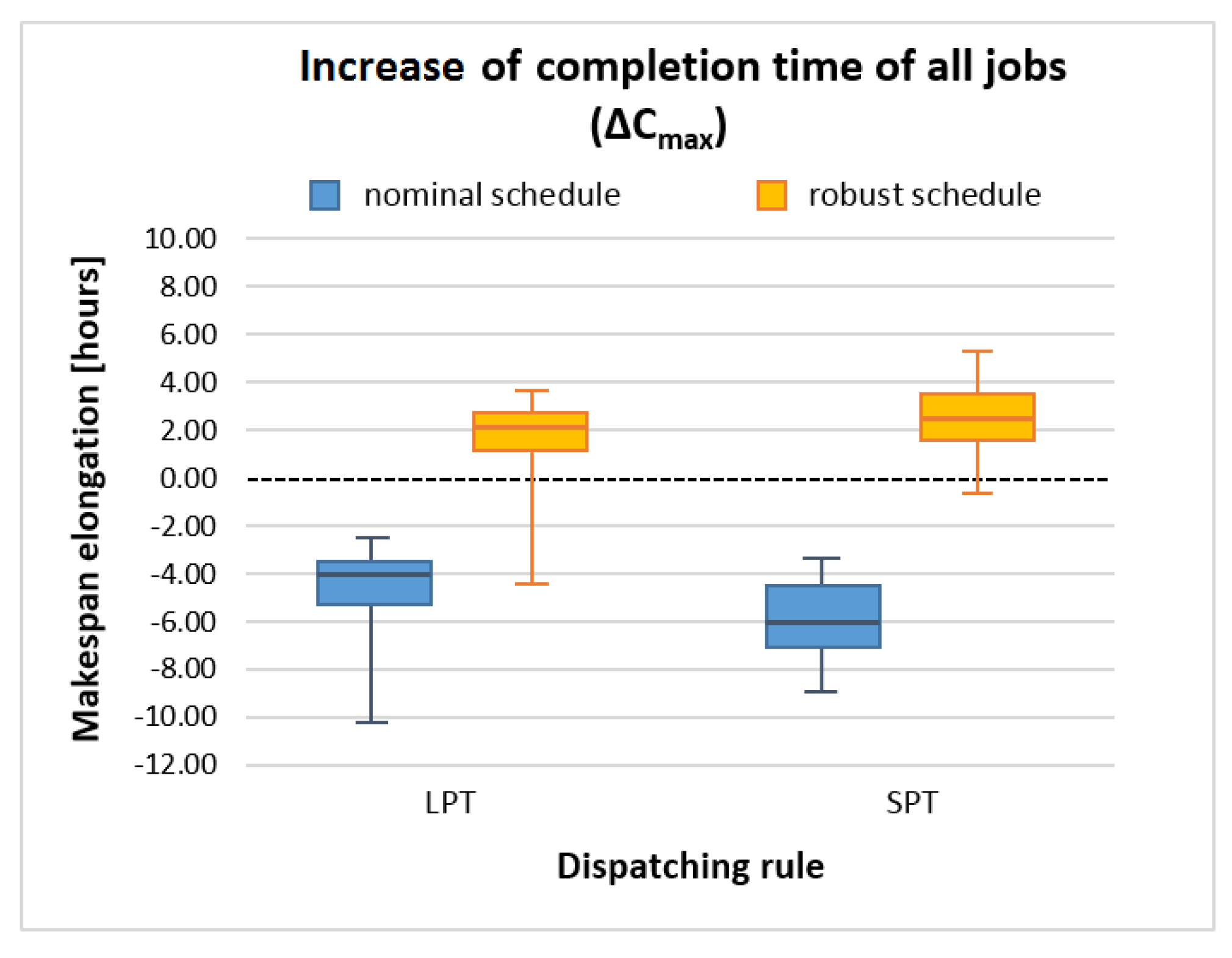
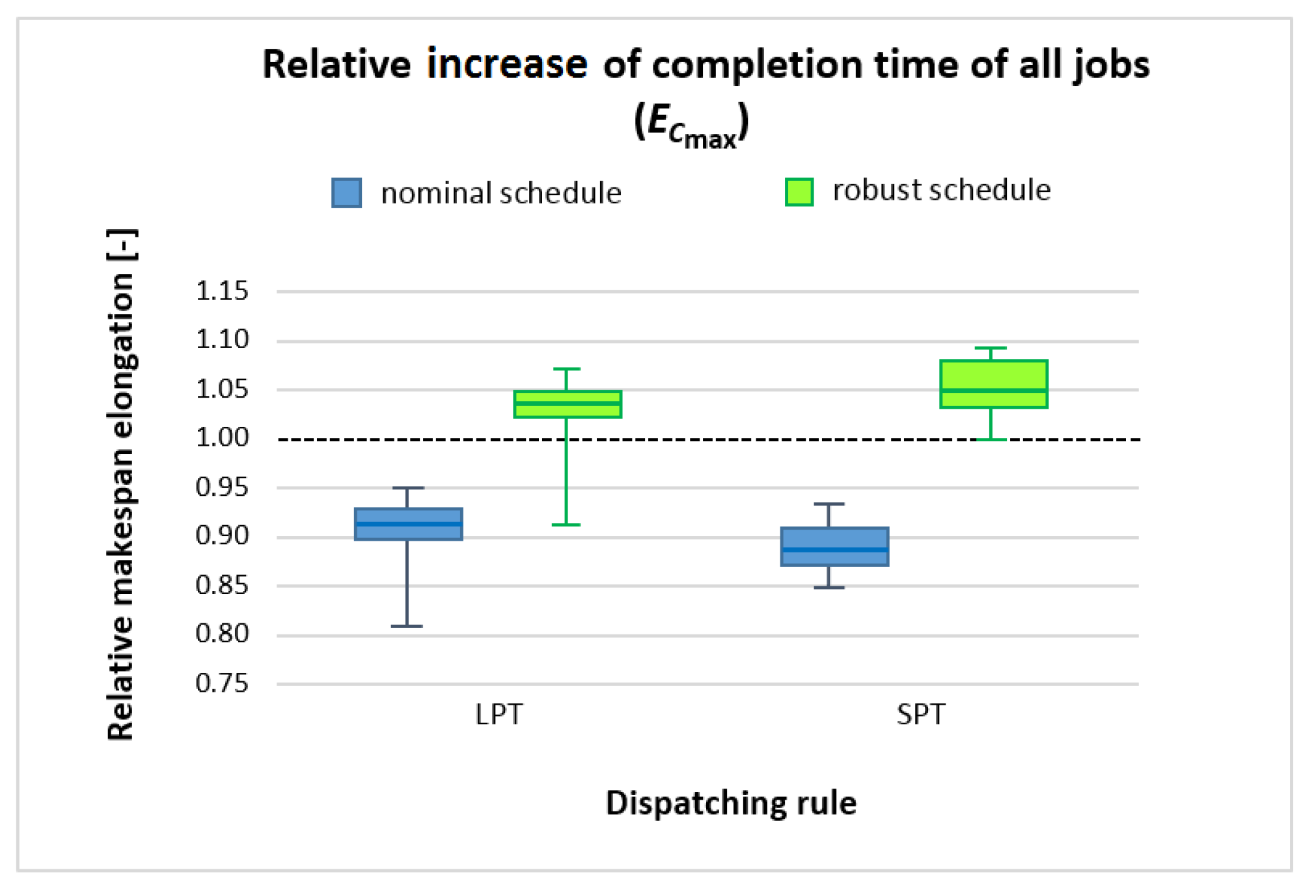
Figure 3 and Figure 4 display the results for makespan increase indicators, which provide further evidence confirming the legitimacy of our solutions. The proximity of the robust schedules to the simulated schedules is again highlighted by their being situated close to the dashed line.

Robust production schedules generated with the application of our solutions determine makespans closer to the simulated completion times of all jobs in the simulated production conditions under technological machinery failure uncertainty. This is evidenced by several indications, e.g., the fact that for the robust schedules, the values of $\Delta C_{\max }$ tend to be close to 0 (Figure 3), whereas in the case of $E_{C_{max}}$ around 1 (Figure 4). Values 0 and 1 of the considered indicators denote igh compliance of the robust schedule with the production execution (simulation).

5. Summary and Conclusions

The execution of production processes is associated with the occurrence of various uncertainty factors. Disruptions generate problems that may have a marked effect on production schedules. Therefore, more effort is required in developing techniques and methods that affirm the relevance of uncertainty factors in manufacturing and propose viable solutions. Robust scheduling exhibits the required potential to cope with disruptions and, thus, should be studied further.

In this investigation, the aim was to design a robust production scheduling method with the implementation of Markov chain theory and ARIMA models that will provide for the negative effects of technological machinery failure. The analyses reveal that the inclusion of machine failure in the production schedule results in the extension of the performance indicators, mean flow time, mean job completion time, as well as the central criterion describing the performance of the production system—the completion time of all jobs (makespan). However, the elongation remains within the reasonable limits given that the production is carried out according to failure-inclusive schedules. The simulations evidence that the robust schedules bear a closer similarity to the simulated production process than their nominal equivalents. In other words, the proposed model generates high-accuracy makespan while increasing the robustness and stability of the schedule.

To extend our research in the future, we intend to develop improved models that will: provide for the management of other uncertainty factors in production scheduling (e.g., disruptions related to transport, availability of materials or employee absence), enable reactive scheduling of production jobs or extend the versatility of the proposed solutions over other manufacturing systems. Our current findings and methodologies should make a noteworthy contribution to the theory of production scheduling, as well as appeal to practitioners representing various manufacturing industries and different-sized enterprises.

References

- Perłowski, R.; Antosz, K.; Zielecki, W. Optimization of the Medium-Term Production Planning in the Company—Case Study. Lect. Notes Electr. Eng. 2018, 505, 369–376. [Google Scholar]
- Burduk, A.; Musial, K.; Kochanska, J. Tabu Search and Genetic Algorithm for Production Process Scheduling Problem. LogForum 2019, 15, 181–189. [Google Scholar] [CrossRef]
- Sobaszek, Ł.; Gola, A.; Kozłowski, E. Application of survival function in robust scheduling of production jobs. In Proceedings of the 2018 Federated Conference on Computer Science and Information Systems (FEDCSIS), Prague, Czech Republic, 3–6 September 2017; Ganzha, M., Maciaszek, M., Paprzycki, M., Eds.; IEEE: New York, NY, USA, 2017; Volume 11, pp. 575–578. [Google Scholar]
- Gürel, S.; Körpeoḡlu, E.; Aktürk, M.S. An Anticipative Scheduling Approach with Controllable Processing Times. Comput. Oper. Res. 2010, 37, 1002–1013. [Google Scholar] [CrossRef] [Green Version]
- Gao, H. Building Robust Schedules using Temporal Potection—An Empirical Study of Constraint Based Scheduling Under Machine Failure Uncertainty. Ph.D. Thesis, Univeristy of Toronto, Toronto, ON, Canada, 1996. [Google Scholar]
- Sobaszek, Ł.; Gola, A.; Kozlowski, E. Job-shop scheduling with machine breakdown prediction under completion time constraint. Adv. Intell. Syst. Comput. 2018, 637, 358–367. [Google Scholar]
- Daniewski, K.; Kosicka, E.; Mazurkiewicz, D. Analysis of the correctness of determination of the effectiveness of maintenance service actions. Manag. Prod. Eng. Rev. 2018, 9, 20–25. [Google Scholar]
- Janardhanan, M.N.; Li, Z.; Bocewicz, G.; Banaszak, Z.; Nielsen, P. Metaheuristic algorithms for balancing robotic assembly lines with sequence-dependent robot setup times. Appl. Math. Model. 2019, 65, 256–270. [Google Scholar] [CrossRef] [Green Version]
- Deepu, P. Robust Schedules and Disruption Management for Job Shops. Ph.D. Thesis, Montana State Univeristy, Bozeman, MT, USA, 2008. [Google Scholar]
- Jasiulewicz-Kaczmarek, M.; Gola, A. Maintenance 4.0 Technologies for Sustainable Manufacturing—An Overview. IFAC PapersOnLine 2019, 52, 91–96. [Google Scholar] [CrossRef]
- Gola, A.; Kłosowski, G. Development of computer-controlled material handling model by means of fuzzy logic and genetic algorithms. Neurocomputing 2019, 338, 381–392. [Google Scholar] [CrossRef]
- Klimek, M. Techniques of Generating Schedules for the Problem of Financial Optimization of Multi-Stage Project. Appl. Comput. Sci. 2017, 15, 20–34. [Google Scholar]
- Rahman, H.F.; Sarker, R.; Essam, D. A Real-Time Order Acceptance and Scheduling Approach for Permutation Flow Shop Problems. Eur. J. Oper. Res. 2015, 247, 488–503. [Google Scholar] [CrossRef]
- Choi, S.H.; Wang, K. Flexible Flow Shop Scheduling with Stochastic Processing Times: A Decomposition-Based Approach. Comput. Ind. Eng. 2012, 63, 362–373. [Google Scholar] [CrossRef] [Green Version]
- Kianfar, K.; Fatemi, G.S.M.T.; Oroojlooy, J.A. Study of Stochastic Sequence-Dependent Flexible Flow Shop via Developing a Dispatching Rule and a Hybrid GA. Eng. Appl. Artif. Intell. 2012, 25, 494–506. [Google Scholar] [CrossRef]
- Almeder, C.; Hartl, R.F. A Metaheuristic Optimization Approach for a Real-World Stochastic Flexible Flow Shop Problem with Limited Buffer. Int. J. Prod. Econ. 2013, 145, 88–95. [Google Scholar] [CrossRef]
- Rahman, H.F.; Sarker, R.; Essam, D. A Genetic Algorithm for Permutation Flow Shop Scheduling Under Make to Stock Production System. Comput. Ind. Eng. 2015, 90, 12–24. [Google Scholar] [CrossRef]
- Chung-Cheng, L.; Kuo-Ching, Y.; Shih-Wei, L. Robust Single Machine Scheduling for Minimizing Total Flow Time in the Presence of Uncertain Processing Times. Comput. Ind. Eng. 2014, 74, 102–110. [Google Scholar]
- Bibo, Y.; Geunes, J. Predictive–reactive scheduling on a single resource with Uncertain Future Jobs. Eur. J. Oper. Res. 2008, 189, 1267–1283. [Google Scholar]
- Jian, X.; Li-Ning, X.; Ying-Wu, C. Robust Scheduling for Multi-Objective Flexible Job-Shop Problems with Random Machine Breakdowns. Int. J. Prod. Econ. 2013, 141, 112–126. [Google Scholar]
- Mehta, S.V.; Uzsoy, R.M. Predictable Scheduling of a Job Shop Subject to Breakdowns. IEEE Trans. Robot. Autom. 1998, 14, 365–378. [Google Scholar] [CrossRef]
- Bierwirth, C.; Mattfeld, D.C. Production Scheduling and Rescheduling with Genetic Algorithms. Evol. Comput. 1999, 7, 1–17. [Google Scholar] [CrossRef]
- Xingquan, Z.; Hongwei, M.; Jianping, W. A robust scheduling method based on a multi-objective immune algorithm. Inf. Sci. 2009, 179, 3359–3369. [Google Scholar]
- Jensen, M.T. Robust and Flexible Scheduling with Evolutionary Computation. Ph.D. Thesis, University of Aarhus, Aarhus, Denmark, 2001. [Google Scholar]
- Janak, S.L.; Lin, X.; Floudas, C.A. A New Robust Optimization Approach for Scheduling Under Uncertainty—II. Uncertainty with Known Probability Distribution. Comput. Chem. Eng. 2007, 31, 171–195. [Google Scholar] [CrossRef]
- Henning, G.P.; Cerda, J. Knowledge-based predictive and reactive scheduling in industrial environments. Comput. Chem. Eng. 2000, 24, 2315–2338. [Google Scholar] [CrossRef]
- Jensen, M.T. Improving robustness and flexibility of tardiness and total flow-time job shops using robustness measures. Appl. Soft Comput. 2001, 1, 35–52. [Google Scholar] [CrossRef] [Green Version]
- Al-Hinai, N.; ElMekkawy, T.Y. Robust and Stable Flexible Job Shop Scheduling with Random Machine Breakdowns Using a Hybrid Genetic Algorithm. Int. J. Prod. Econ. 2011, 132, 279–291. [Google Scholar] [CrossRef]
- Davenport, A.; Gefflot, C.; Beck, C. Slack-based Techniques for Robust Schedules. In Proceedings of the Sixth European Conference on Planning, Toledo, Spain, 12–14 September 2001. [Google Scholar]
- Kempa, W.; Paprocka, I.; Kalinowski, K.; Grabowik, C. Estimation of reliability characteristics in a production scheduling model with failures and time-changing parameters described by Gamma and exponential distributions. Adv. Mater. Res. 2014, 837, 116–121. [Google Scholar] [CrossRef]
- Kempa, W.; Wosik, I.; Skołud, B. Estimation of Reliability Characteristics in a Production Scheduling Model with Time-Changing Parameters—First Part, Theory. Manag. Control Manuf. Process. 2011, 1, 7–18. [Google Scholar]
- Rosmaini, A.; Shahrul, K. An overview of time-based and condition-based maintenance in industrial application. Comput. Ind. Eng. 2012, 63, 135–149. [Google Scholar]
- Rawat, M.; Lad, B.K. Novel approach for machine tool maintenance modelling and optimization using fleet system architecture. Comput. Ind. Eng. 2018, 126, 47–62. [Google Scholar] [CrossRef]
- Baptista, M.; Sankararaman, S.; De Medeiros, I.P.; Nascimento, C.; Prendinger, H.; Henriques, E.M.P. Forecasting fault events for predictive maintenance using data-driven techniques and ARMA modeling. Comput. Ind. Eng. 2018, 115, 41–53. [Google Scholar] [CrossRef]
- Kalinowski, K.; Krenczyk, D.; Grabowik, C. Predictive-reactive strategy for real time scheduling of manufacturing systems. Appl. Mech. Mater. 2013, 307, 470–473. [Google Scholar] [CrossRef]
- Sobaszek, Ł.; Gola, A.; Kozłowski, E. Module for prediction of technological operation times in an intelligent job scheduling system. In Intelligent Systems in Production Engineering and Maintenance—ISPEM 2018: International Conference on Intelligent Systems in Production Engineering and Maintenance; Burduk, A., Chlebus, E., Nowakowski, T., Tubis, A., Eds.; Springer: Cham, Switzerland, 2018; pp. 234–243. [Google Scholar]
- Knopik, L.; Migawa, K. Semi-Markov system model for minimal repair maintenance. Eksploat. I Niezawodn. Maint. Reliab. 2019, 21, 256–260. [Google Scholar] [CrossRef]
- Stewart, W.J. Probability, Markov Chains, Queues, and Simulation; Princeton University Press: Princeton, NJ, USA, 2009. [Google Scholar]
- Ross, S. Introduction to Probability Models, 6th ed.; Academic Press: San Diego, CA, USA, 1997. [Google Scholar]
- Kozłowski, E.; Borucka, A.; Świderski, A. Application of the logistic regression for determining transition probability matrix of operating states in the transport systems. Eksploat. I Niezawodn. Maint. Reliab. 2020, 22, 192–200. [Google Scholar] [CrossRef]
- Chow, G.C. Ekonometria; PWN: Warszawa, Poland, 1995. [Google Scholar]
- Kozłowski, E. Analiza i Identyfikacja Szeregów Czasowych; Politechnika Lubelska: Lublin, Poland, 2015. [Google Scholar]
- Box, G.E.P.; Jenkins, G.M. Time Series Analysis: Forecasting and Control. Holden-Day; Wiley: San Francisco, CA, USA, 1970. [Google Scholar]
- Rymarczyk, T. Characterizations of the shape of unknown objects by inverse numerical methods. Prz. Elektrotechniczny 2020, 88, 138–140. [Google Scholar]
- Kozłowski, E.; Mazurkiewicz, D.; Żabiński, T.; Prucnal, S.; Sęp, J. Machining sensor data management for operation-level predictive model. Expert Syst. Appl. 2020, 159, 113600. [Google Scholar] [CrossRef]
- Shumway, R.H.; Stoffer, D.S. Time Series Analysis and Its Applications with R Examples; Springer: Cham, Switzerland, 2017. [Google Scholar]
- Kosicka, E.; Kozłowski, E.; Mazurkiewicz, D. The use of stationary tests for analysis of monitored residual processes. Eksploat. I Niezawodn. Maint. Reliab. 2015, 17, 604–609. [Google Scholar] [CrossRef]
- RStudio Team. RStudio: Integrated Development for R; PBC: Boston, MA, USA, 2020; Available online: http://www.rstudio.com (accessed on 10 July 2020).
- Bräsel, H.; Dornheim, L.; Kutz, S.; Mörig, M.; Rössling, I. LiSA—A Library of Scheduling Algorithms; Magdeburg University: Magdeburg, Germany, 2001. [Google Scholar]
- Chiang, T.C.; Fu, L.C. Using Dispatching Rules for Job Shop Scheduling with Due Date-Based Objectives. Int. J. Prod. Res. 2007, 45, 1–28. [Google Scholar] [CrossRef]
Figure 1.
Markov chains with transition diagrams for the considered machines: (a) Machine M1; (b) Machine M2; (c) Machine M3; (d) Machine M6; (e) Machine M7; (f) Machine M8.
Figure 2.
Schedules obtained using the SPT (shortest processing time) rule: (a) nominal, (b) robust.
Figure 3.
Increase of makespan in LPT and SPT schedules.
Figure 4.
Relative increase of makespan in LPT and SPT schedules.