On the Statistical Characterization of Sprays


1
ADAI, LAETA, Mechanical Engineering Department, University of Coimbra, Rua Luis Reis Santos, 3030-788 Coimbra, Portugal
2
IN+, Mechanical Engineering Department, Instituto Superior Técnico, University of Lisbon, Av. Rovisco Pais, 1049-001 Lisboa, Portugal
3
CINAMIL, Department of Exact Sciences and Engineering, Portuguese Military Academy, Rua Gomes Freire, 203, 1169-203 Lisboa, Portugal
*
Author to whom correspondence should be addressed.
Appl. Sci. 2020, 10(17), 6122; https://0-doi-org.brum.beds.ac.uk/10.3390/app10176122
Submission received: 10 August 2020
/
Revised: 28 August 2020
/
Accepted: 29 August 2020
/
Published: 3 September 2020
(This article belongs to the Special Issue Progress in Spray Science and Technology)
Abstract
:Featured Application
The work establishes the grounds for the spray characterization using statistical analysis, how to explore it to improve the physical interpretation of spray processes, and advance the methods to report it in a way that further advances spray science.
Abstract
The statistical characterization of sprays is an essential way of organizing data on drop size and velocity to provide reliable information on the spray dynamics. A clear presentation of data using statistical tools provides evidence of a clear research question underlying the spray characterization. In this article, a review of the best practices to build histograms is presented, as well as three relevant details on spray characterization: (i) the application of information theory to assess if we have enough information (not data); (ii) the link between mathematical probability distributions and the physical interpretation of spray data; (iii) and introducing, for the first time, the concept of drop size diversity, with the quantification of the polydispersion and heterogeneity degrees. Finally, the view presented is applied to the characterization of nanofluid sprays for thermal management.
1. Introducing the Statistical Organization of Spray Data
A spray is a two-phase flow of droplets interacting with a gaseous continuous phase. The physical process of liquid atomization depends on the atomizer type and breakup process, and once completed, the droplets formed have multiple sizes and velocities, and statistical histograms are the most common way of organizing the large amount of data on their characteristics.
In the sense of data organization, the histograms organizing the sizes and velocities of droplets by classes do not represent a probability of occurrence, as in conventional statistical analysis, but a probability of presence of droplets in a spray, since the atomization mechanisms already occurred. This small language shift allows considering each probability value as representing the degree of relevance of a certain class in the spray—a notion which will be essential to understand drop size diversity.
In practice, after sorting data by classes, the way histograms represent the probability of presence is dividing the counts in each class () by the total sample size (N), . However, if there is a need to increase the detail of the distribution, one can build the discrete distribution in terms of density of probability of presence by considering the bin width () in the probability value as . The bin width is constant if size classes are regularly spaced within the spectrum, or can vary the size if irregularly spaced.
In the case of discrete probability distributions, the sum of all probability values associated with each class k is equal to one, , which means that each probability value corresponds to the weight a number of drops within a characteristic class k has in the entire spray. It is why one designates this way of presenting spray data as a number-weighted probability distribution. There are other ways as shown later.
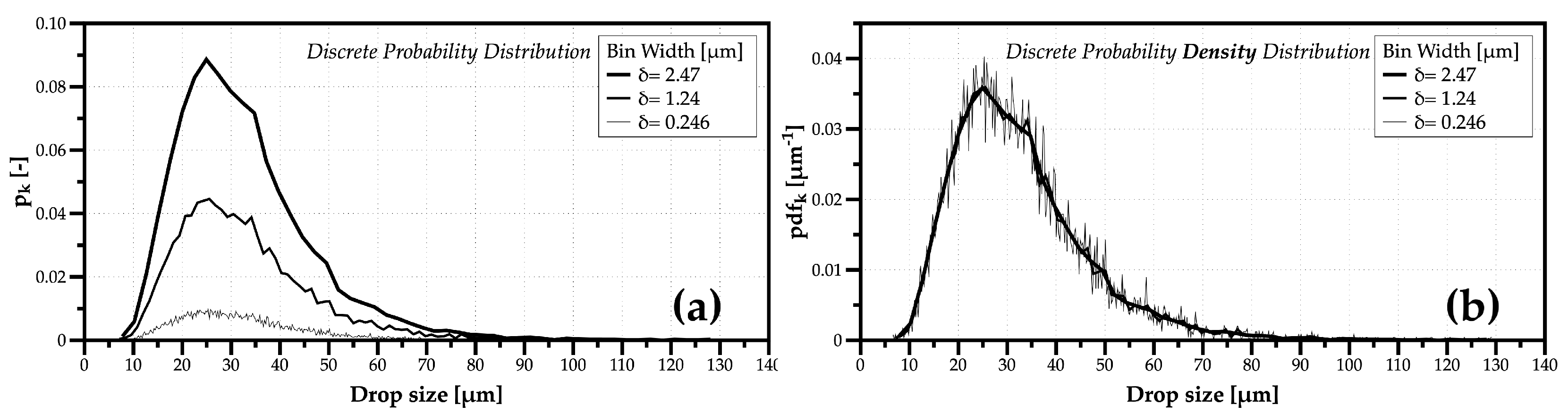
The interpretation of the probability as a number-weighted value of class k, for example, applied to drop sizes , allows for calculating the moments of the size distribution, such as the average size of droplets, , whether using a probability discrete distribution or a probability discrete density distribution, respectively. Although this is basic statistical knowledge, in several research works, it is unclear which is the distribution reported, considering that each approach (probability or probability density) reacts differently when we increase the detail of a distribution by changing the bin width , as illustrated in the example of Figure 1.
While a smaller bin size implies a higher number of classes, in probability distributions, it leads, ultimately, to a uniform probability distribution with one class per sample (Figure 1a). However, in probability density distributions, it increases the detail to allow identifying eventual multimodalities dues to different drop cluster with similar characteristics, or increase the noise in values, as illustrated in the examples depicted in Figure 1b.
The purpose of remarking the difference between probability and probability density distribution is particularly relevant when comparing experimental with simulated drop characteristics. In the case of using a probability distribution (), the number of classes must be the same, or the representative values of each class ( for drop size and for one velocity component). Otherwise, if the presentation of spray data opts for the probability density distribution, which is dimensional ( [m]), it is not necessary to use the same number of classes. Ultimately, to avoid erroneous comparisons between experimental and simulated data, it is essential to be clear about the approach followed when presenting spray data in statistical format. The question is why one should change or tune the number of classes when describing the spray characteristics.
The underlying idea of increasing the number of classes is to obtain a greater detail of the probability distributions and detect eventual multimodality associated with clusters of data with dissimilar characteristics. In the case of drop sizes, an example generating such multimodality would be the presence of multiple atomization mechanisms (e.g., aerodynamic and/or hydrodynamic). In addition, in the case of the velocity, different two-phase flow events like the impact of droplets on solid surfaces contain information about the axial velocity component with positive values from those impinging on the surface, but the secondary droplets resulting after impact have a negative velocity component. Therefore, what is the criterion for choosing a given number of classes, k? In addition, should the spacing of these classes be regular or irregular?
Considering regularly spaced classes, one of the basic principles introduced by Sturges [1] stated that the number of classes , with N as the total sample size. Doane [2] further elaborated on Sturge’s rule, but the problem is the over-smoothing of histrograms produced and its applicability limited to a number of data samples below 200, as analyzed by Hyndman [3]. The alternatives for the Sturge’s and Doane’s rules are the:
Considering a simulated example of two clusters of droplets, each following a lognormal distribution function
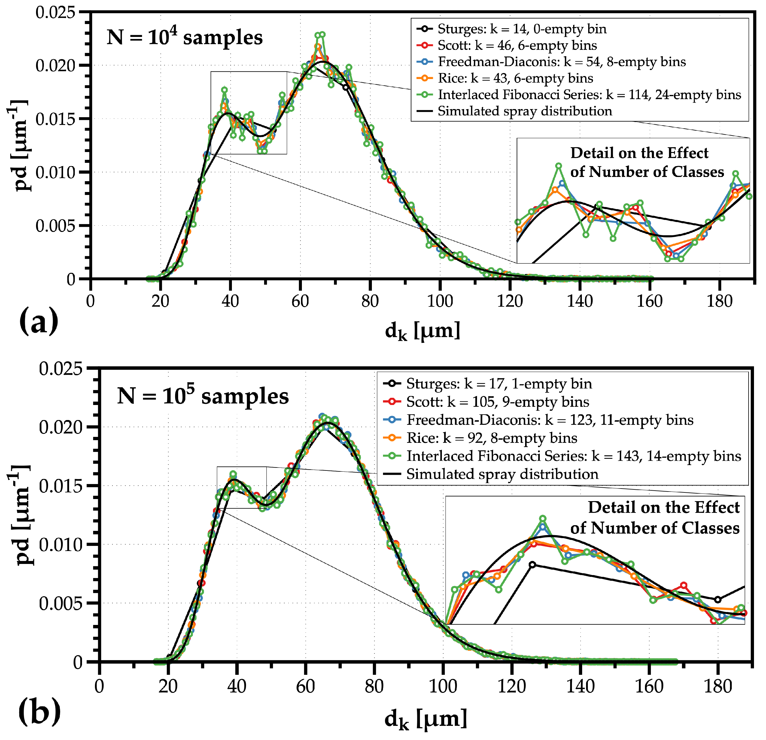
with as the geometric diameter and as the geometric standard deviation, the final distribution function is a mixture between the two as with . Figure 2 shows the effect of using different criteria to organize drop size data with (a) N = 10 and (b) N = 10 measurements in the form of probability density distributions of drop size.
For the two sample sizes tested, the Sturges’ rule clearly over-smooths the distribution’s bimodality. The Scott’s rule generates less classes but is enough to capture the multimodality of the drop size distribution while producing the minimum number of empty classes. The Freedman and Diaconis proposal, and the interlaced Fibonacci series, can provide greater detail, but the results with the lower number of samples (Figure 2a) prove the cost of increasing the number of classes by a larger noise observed in probability density values. It is noteworthy that the best approach to represent drop size distributions for comparison purposes is a probability density ( [m), since the amplitude of distributions with a different number of classes does not change as the amplitude of probability distributions ().
The second approach to define classes in drop size statistics (less so in velocity) is the use of irregular bin widths. For example, in laser diffraction measurement systems, like Malvern’s Spraytec, the ratio is constant, leading to broader classes for larger diameters representing each class. However, a systematic method for using irregular bin width to improve the description of drop size and velocity distributions is still open for further research. These details seldom appear reported in the literature when authors present the results of spray characterization and compare sprays obtained in different operating conditions. In this sense, the approach less prone to error would be to present the statistical data of the spray characteristics in terms of cumulative probability distributions, as explored later in this introduction.
A final remark on the presentation and analysis of spray data in the form of statistical distributions is to consider the weight given to each class. In the case of the velocity of spray droplets, a number-weighted probability distribution is the most adequate. However, for histograms of drop size, other weighting factors, such as the
- area-weighted
- with and ;
- and volume-weighted
- with and ;
applied to probability distributions improve the interpretation of its moments, as reported in the work of Sowa [8]. The reason for organizing spray data with other weight values besides the number-weighted case relates to the physics associated with the research question. Namely, if the investigation involves phenomena occurring at the droplet surface area, such as heat and mass transfer events, an area-weighted drop size distribution is more adequate. However, if the spray liquid volume is more important, such as spray cooling applications, the most adequate is the volume-weighted drop size distribution.
The characterization of a spray often involves moments of the measured discrete probability distribution using single-point diagnostic techniques, like the Phase-Doppler Interferometry, or field diagnostic techniques using imaging. In the case of drop size, the calculation of each moment from drop size raw data corresponds to
where is a measurement of drop size in the sample acquired. If these moments use, instead, the number-weighted probability distribution values, the expression is
with as the number of measurements counted within the size class k where represents the mid-point in the interval between a lower and an upper bound.
The characterization of the spray droplets using the average size obtained from a number-weighted probability distribution——means considering all droplets have, on average, the same size of . For example, when comparing for different locations in the spray, or the same location for different sprays, any increase implies more droplets of larger sizes. When analyzing the physics of droplet transport while interacting with the surrounding environment, the arithmetic mean diameter might be a valuable characteristic measure to consider. However, when the research aims at combustion applications, with evaporation and mass diffusion phenomena occurring at the surface area of each droplet, the best characteristic size is , since it is the average of an area-weighted probability distribution—or else, if the research points to spray cooling applications, where the mass deposited on the surface is the relevant parameter due to its contribution to the formation of liquid films and their dynamic behavior, the best characteristic size for analyzing the heat and mass transfer involved would be , the average of a volume-weighted probability distribution.
The main point when choosing the best way to present spray data is the awareness that each characteristic parameter, obtained statistically, has an underlying physical meaning, depending on the thermofluid phenomena involved. Finally, it is noteworthy that providing the moments of drop size and velocity distributions may limit the use of spray data in future works and spray simulations because of the inability to reconstruct the original distributions from the moments reported. Therefore, the next section discusses the implications for spray science of the attempt to fit a probability distribution functions to the histograms of drop size.
2. Drop Size Distribution Functions and Spray Science
Spray characterization provides relevant information of droplets dynamics for the application of its mean quantities in empirical correlations related with heat transfer and fluid flow processes. The several optical diagnostic techniques acquire large amounts of data and the challenge is often how to process it. The criterion for the sample size (N) of spray data recurs often to the notion of statistical uncertainty. When its value is below a pre-defined threshold, the measurement stops because the experimentalist has enough data. However, this criterion often interprets spray data as a random probabilistic event, while spray statistics is more a method for organizing data. Therefore, the right question is not whether there is enough data to post-process and characterize a spray, but whether there is enough information. Section 2.1 reviews an approach based on information theory to make this assessment.
Secondly, the meaning of using an average quantity to describe a spray, where droplets have multiple sizes, is to assume that whatever physical phenomenon affects an average size represents what occurs to the entire spray. The limitation of presenting the spray data based solely on mean quantities is the loss of information of the local or global drop polydispersed sizes or velocities in the spray and its potential usefulness in the development of numerical models that simulate sprays. However, while it is difficult to retrieve information of the original statistical distributions from their mean quantities, the ability to reconstruct drop size or velocity distributions from characteristic parameters of the mathematical probability distribution functions (), instead of its moments, allows for obtaining the mean quantities without losing the information of the original distributions. Therefore, approaching spray characterization from the point of view of reconstructing probability distributions has significant advantages over the approach that uses solely moments retrieved from discrete probability distributions that describe a spray (e.g., see Panao and Radu [9]). Section 2.2 reviews the fitting of probability distribution functions to histograms of drop data to retrieve the characteristic parameters allowing the reconstruction of spray data distributions, but introduces the argument of whether or not such fitting can provide some insight into the physics of the atomization process.
The final Section 2.3 introduces, for the first time, the notion of drop size diversity, distinguishing the polydispersion degree from the heterogeneity degree and presenting the best parameters for their characterization. An accurate characterization of drop size diversity is relevant for the design of sprays.
2.1. Defining Enoughness in Large Data Samples
An experimentalist stops a measurement based of criteria related to a statistical uncertainty. The definition of statistical uncertainty contains three conditions:
- it is maximum for a uniform distribution where all classes have the same probability;
- a small variation in the probability of a class generates a small variation in the uncertainty;
- and, finally, it depends on the distribution itself.
The common measure used for the statistical uncertainty considers the standard deviation ( ) and the sample size (N) as
with as the coefficient associated with the confidence interval considered (e.g., for a 95% Confidence Interval). When the mean value () is different from zero, dividing by the mean provides the uncertainty in percentage. Since the standard deviation depends on the spray characteristics, reducing the statistical uncertainty implies adding more data to increase N. However, as argued by Panao [10], if the spray begins to operate in a different way and the distribution changes, the statistical uncertainty as defined in Equation (4) continues to decrease, without providing any evidence to the experimentalist about the changes occurring in the spray. In a certain sense, it fails to comply to the third condition defining a statistical uncertainty because it is more sensitive to the sample size than the distribution itself. For this reason, an approach based on information theory is a better option.
In information theory, the Shannon entropy complies to all the aforementioned characteristics of a statistical uncertainty. Considering the probability values of any discrete distribution (), the expression for calculating the Shannon entropy H is
As an example, if we consider drop size, the minimum value corresponds to a monosize spray with all droplets having the same size, thus, , and . The maximum value occurs for a hypothetical spray where all droplets have the same probability of being present, corresponding to a uniform distribution with k classes, each for a different drop size. Therefore, the maximum Shannon entropy is . In sprays, while measuring size and velocity, considering the Shannon entropy normalized by its maximum value, , it tends to stabilize (see Panao [10] for details). The meaning is that adding more data does not mean adding more information because the shape and scale of the distribution stabilized. However, as argued in Panao [10], the enoughness requires a criterion with interpretative value and proposes the excess entropy () because, as defined in Feldman et al. [11], it is what best captures the nature of convergence of the entropy rate as the amount of memory gained, or the cost of amnesia if all data would suddenly be lost. To evaluate the evolution of while measuring,
- one calculates the entropy rate that quantifies the difference between the normalized Shannon entropy with adding one value the N samples and the Shannon entropy with N samples-;
- considers the limit when , which is ;
- and the excess entropy is formulated as
In the case of spray data, the stabilization implies = 0, thus, it simplifies . The method proposed is setting a convergence criterion– and stop measuring when , considering the number of samples corresponding to the median as the minimum required (see Panao [10] for more details).
Once the experimentalist has enough information and organizes the spray data with histograms of drop velocity and weighted distributions of drop sizes, depending on the physical process under analysis, one of the methods to avoid losing information of the measured distributions is fitting data to known mathematical or empirical distribution functions. However, the question is whether such fitting can provide further insight into liquid atomization mechanisms. This is the topic explored in the next sub-section.
2.2. Underlying Physics of Probability Distribution Functions Applied to Sprays
An important consideration when characterizing sprays is the effect of the interaction between droplets and the continuous phase on the local (or even overall) size and velocity distributions. This interaction involves different transport phenomena, with momentum and energy exchanges between the dispersed phase (spray) and the carrier phase (surrounding environment), generating eventual secondary breakup of the spray droplets leading to changes in the shape and scale of drop size distributions, or acceleration (positive or negative) captured by changes in local velocity probability distributions. However, the physical reason why a certain distribution function might fit better than another is still open for further research.
This work advances an argument in favor of distinguishing between modeling and characterizing drop size distributions. The purpose of modeling drop size distributions is to predict them from the information of the atomizer geometry and operating conditions. The simulation of sprays using a numerical approach [12], or a statistical or stochastic approach [13] can produce data on the droplets characteristics, but it is different from statistically processing such data. Therefore, according to Déchelette et al. [14], there are four methods for modeling drop size distributions:
- the empirical;
- the Maximum Entropy Formalism (MEF);
- the Discrete Probability Function (DPF);
- and the Stochastic.
However, the purpose of characterizing a spray is to describe, as accurately as possible, the polydispersion of sizes and velocities of its droplets. This description aims at obtaining mean quantities for analyzing heat transfer and flow processes—or its aim is to improve our understanding of the nature underlying the atomization mechanisms.
There are two categories of probability distribution functions used to describe droplets’ characteristics: mathematical and empirical. Lefebvre and McDonell [15] provide a synthesis of the main probability distributions in each category. Except for the Rosin–Rammler or Weibull, the Nukiyama–Tanasawa and Upper-Limit empirical distribution functions are complex and problems arise when determining the best-fit values for their parameters. As to the mathematical distribution functions, the simplest is the Log-Normal, while the Log-Hyperbolic is also complex and problems arise with finding the best fitting parameters. One distribution absent from Lefebvre and McDonell [15] and other review works is the Gamma distribution function which Villermaux et al. [16] associated with the distribution of droplets resulting from the fragmentation of ligaments, generating a spray, reviewed later in this section.
While most research on spray characterization focuses on the fitting process, few works such as Villermaux [17] and Villermaux et al. [16] address the meaning of the mathematical distribution function used and the physical background for such fitting. As mentioned in the Introduction, instead of focusing our attention on probability or probability density functions, we propose a greater focus on cumulative distribution functions (). Therefore, any comparison between different becomes universal and if such distribution properly describes the local or global experimental results, its digitization to simulate a spray is relatively accessible.
In the case of the Log-Normal distribution, its cumulative form given by
includes as the scale parameter, the geometric mean diameter, and as the shape parameter of the distribution. Applied to spray characterization, the reason for using a Log-Normal distribution function is related to the multiplicative effect of subsequent stages of droplets breaking up during atomization, as a cascade process, where one drop breaks into two or more and so on. However, if we consider the interaction between droplets and the continuous gaseous phase, in time, the dragging of droplets leads to secondary flows which eventually produce a vortical effect on the transport of subsequent droplets. Namely, smaller droplets, with lower response times, dragged by secondary flows, may return to upward locations, redistributing the counts of certain drop size classes in locations further downstream of the spray trajectory. Therefore, even if it is not the result of a multiplicative breakup process, the presence of these smaller drops affects the probability distributions describing the spray, having an effect similar to that of a cascade of multiple breakup stages. One could even speculate whether or not the reason for a Log-Normal distribution best fitting experimental results expresses the way the multiphase flow organizes the transport of droplets according to their size in a cascade pattern.
Besides several breakup stages and transport phenomena, some atomization processes result from the disintegration of liquid sheets or jets into ligaments, and those ligaments further fragmenting into droplets. In this case, Villermaux et al. [16] argues each ligament constituted of several blobs, and when it fragments into several droplets, the size distribution that reasonably fits is a Gamma probability distribution function, which cumulative form is expressed by
with a and b as the shape and scale parameter, respectively. In this case, a characteristic size corresponds the product of both: .
Considering empirical distribution functions, this work focuses on the Weibull distribution, first applied to describe the distribution of drop sizes by Rosin and Rammler,
where is a scale parameter related to a characteristic drop size and q is the shape parameter and considered a measure of the spreading in drop sizes. The accuracy of this empirical probability distribution is best related to drop size distributions with fewer smaller droplets or narrower size distributions [15].
A final note considers the Nukiyama–Tanasawa empirical distribution that is often used to fit experimental data. Here, particular attention is given to the work of Li and Tankin [18] that derived the expression using an information-theory approach, and for the spray liquid volume, its cumulative form results in
where q is also the shape parameter.
The average quantities referred to so far are related to moments in probability distributions, but considering the cumulative distribution, any quantity corresponds to a representative diameter, generally expressed as , where x is the type of distribution, and w is the percent cumulative value related to the representative diameter. Therefore, if the cumulative distribution is
- number-based, represents the size containing w% of the droplets in the spray;
- area-based, represents the size containing w% of the spray surface area;
- volume-based, represents the size containing w% of the liquid spray volume.
One of the most relevant representative diameters corresponds to 50% (, or ) because dividing the classes by that number allows a better comparison between cumulative distributions, useful for analyzing the effect of parametric variations in the spray.
2.3. Introducing Drop Size Diversity in a Spray
Drop size distributions are a way to organize the data acquired to characterize a spray. The characterization of the diversity of drop sizes answers two distinct questions: (1) how many different sizes are relevant in a spray; (2) and how different are the relevant sizes in a spray. The word relevant links to the probability of presence of certain drop size classes relative to others.
In the known textbook on Atomization and Sprays, Lefebvre and McDonell [15] refer to this diversity as drop spray dispersion associated with the size range of droplets. On the other hand, several research articles address the different sizes of the spray droplets as a polydispersed spray. In the authors’ opinion, these are two different things, which is why we introduce the concept of Drop Size Diversity (DSD) measured by two different degrees:
- the polydispersion degree to quantify the multitude of different sizes that are relevant in a spray. Thus, the maximum for the case where all different sizes have the same probability of being present in the spray, and
- the heterogeneity degree to quantify how different are the relevant sizes in the spray. Therefore, it is related with the size range or size dispersion.
The challenge is to devise the right indicators to measure both degrees. Among the several indicators available and synthesized in Lefebvre and McDonell [15], the most known and used indicator is the Relative Span obtained from the representative diameters of a volume-based cumulative size distribution ( with as the fraction of the spray liquid volume) as
Considering the normalization of a representative diameter by the value representing half of the liquid volume--as , the interpretation of Equation (10) relative to the range of drop sizes corresponds to a difference- which is equal to zero when all droplets in the spray have the same size, and maximum when all droplets have the same probability of occurrence (a limit unrealistic case).
Panao [19] proposed a different approach based on information theory, through the concept of the normalized Shannon entropy, already defined in Section 2.1 as
In the information theory terminology applied to spray characterization, a spray where all droplets have the same size, , resulting in a null normalized Shannon entropy, , while an unrealistic spray with all classes having the same probability of presence (uniform distribution), , because the Shannon entropy–numerator in Equation (11)–is maximum.
Finally, García et al. [20] proposed a third approach based on the standard deviation of the volume-weighted drop size distribution expressed as
where and are the second- and first-order moments of the volume-weighted drop size distribution, respectively. The authors compared this standard deviation with Shannon entropy and found inconsistencies. They state that the Shannon entropy has a main drawback, since the information of the drop sizes representing each class is not explicitly included; thus, if these probability values would be randomly rearranged, the H value would be the same. This is an important insight because it allows to understand the difference between polydispersion and size dispersion in a spray.
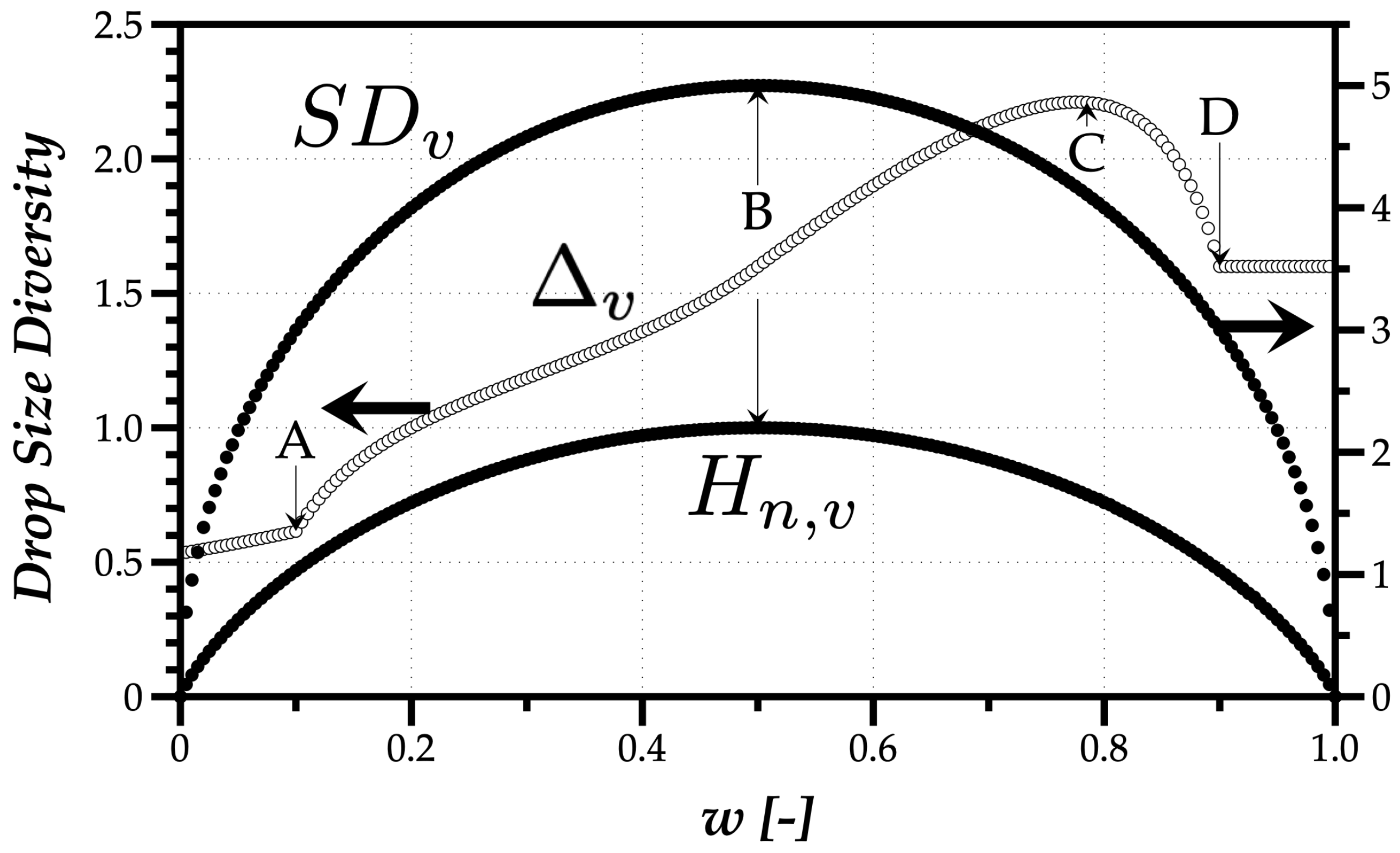
To compare the three approaches, consider the simulation of a spray mixing two monosize droplet streams of m and m. A weight parameter w, varying between 0 and 1, sets the percentage of drops present in the mixed spray from each of the monosize sources. Therefore, if , all droplets have the size of m, and if , all droplets have m. Figure 3 shows the result for the Relative Span (), normalized Shannon entropy based on the volume-weight drop size distribution (), and the volume-weighted standard deviation () with the variation of the weight w attributed to the presence of droplets from each monosize source.
In the extreme cases where all droplets have the same size, the absence of polydispersed sizes results in null values for all indicators. However, while a small portion of droplets of a different size leads to a discontinuity in , the normalized Shannon entropy and the volume-weighted standard deviation show a continuous behavior. In Figure 3, points A and D in mark the limits of 10% and 90% of the spray volume, meaning until A, 10 m droplets do not make 10% of the spray volume, and, at point D, these small droplets reached the mark of 90% of the spray volume. The maximum value of at point C has no evident meaning.
The evolution of is simple to interpret. The maximum normalized Shannon, , occurs when all droplets have the same probability of being present in the spray (), corresponding to the uniform distribution. It is noteworthy that has no discontinuities as , and the variation with w shows a transition between the monosize spray droplets with m to the monosize spray of m droplets. It means that the size of droplets has no influence on , only their relevancy in the spray. On the contrary, the volume-weighted standard deviation depends on the maximum distance between relevant drop size in the spray. In this case, with an evolution similar to , the maximum occurs at m corresponding to the maximum distance between a mean quantity (15 m) and the sizes of the monodispersed sprays (10 and 20 m).
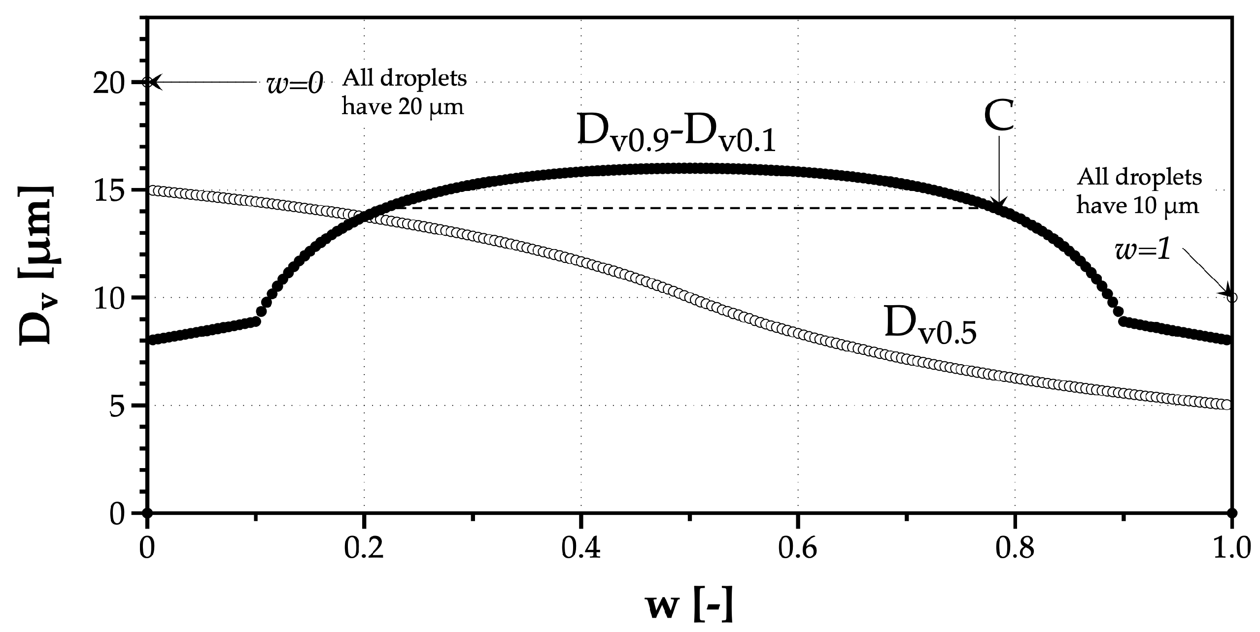
The Relative Span raises several questions, eventually pointing to its limitation if used to quantify the droplets size diversity. Namely, the values depend on drop sizes. Why would a monosize spray of smaller droplets, with a small portion of a monosize spray of larger droplets have a higher Relative Span? In fact, Figure 4 helps to understand why this outcome is a result of the evolution of the diameter representing 50% of the liquid volume of the spray ().
The first observation from Figure 4 is the similarity between the other indicators () and the evolution of the difference D–D, in the numerator of , as a function of w with a maximum value at . However, because the relative span normalizes this difference by , which continues to decrease as the number of 10 m droplets in the mixed spray increases, grows and indicates, for no reason, an increase of the drop size diversity until point C, when it is not the case. This theoretical example shows the limitations of using the relative span as a reliable tool to quantify the drop size diversity in a spray.
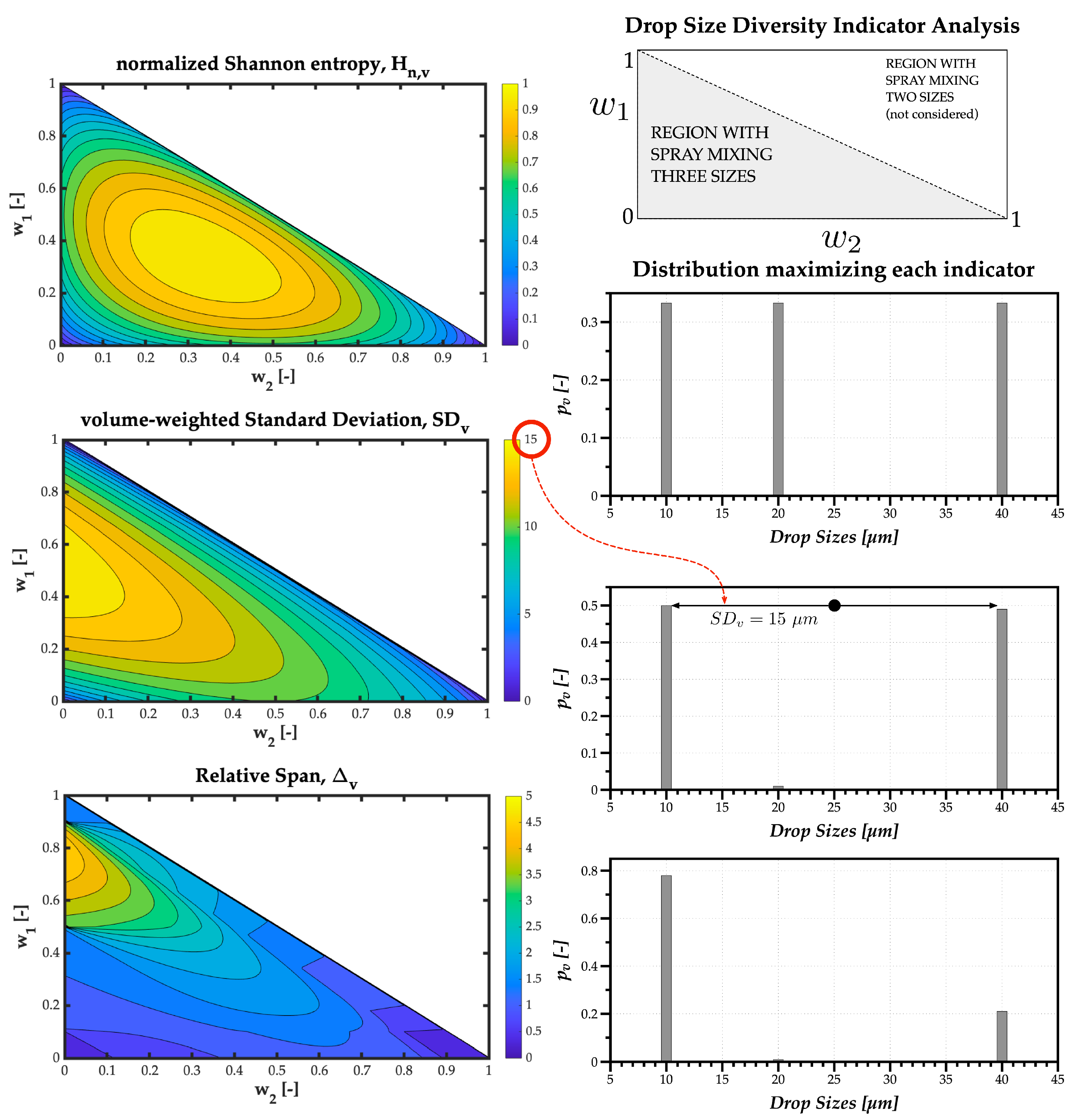
Although for the previous example, the and led to the same value of w = 0.5 corresponding to the maximum polydispersion and heterogeneity degrees, the parameters express different meanings relative to the drop size diversity. Therefore, a second theoretical simulation uses three monosize stream of droplets with 10, 20, and 40 m, with weights , and , respectively, varying from 0.01 to 0.98 to ensure that a percentage of all three sizes, no matter how small, is present in the spray.
Figure 5 shows the contour plots for each Drop Size Diversity indicator as a function of and , and plots on the right are the distributions corresponding to the maximum value obtained by each indicator. This simulation clarifies the difference between the polydispersion and heterogeneity degrees. Namely, the maximum normalized Shannon entropy obtained for the maximum number of droplets relevant in the spray corresponds to the uniform distribution where all relevant drop sizes have the same probability of being present in the spray—thus an adequate parameter to quantify the polydispersion degree.
The results for the volume-weighted standard deviation prove a maximum for the maximum difference between relevant drop sizes. In this case, between 10 m and 40 m droplets, with the standard deviation value of 15 m relative to the mid-point around 25 m—thus an adequate parameter to quantify the heterogeneity degree.
The results for the relative span show its meaning is closer to the heterogeneity degree, expressed by previous authors as size dispersion. However, it is a limited parameter to evaluate Drop Size Diversity, as shown by the distribution representing its maximum value closer to 5, which is difficult to interpret.
The next step would be to simulate a spray resulting from the mixture of two polydispersed sprays, for example, using the Log-Normal distribution with different geometric mean diameters () and equal shape parameters (see Equation (1)), and change the mixing through the weight parameter w to simulate the transition between distributions.
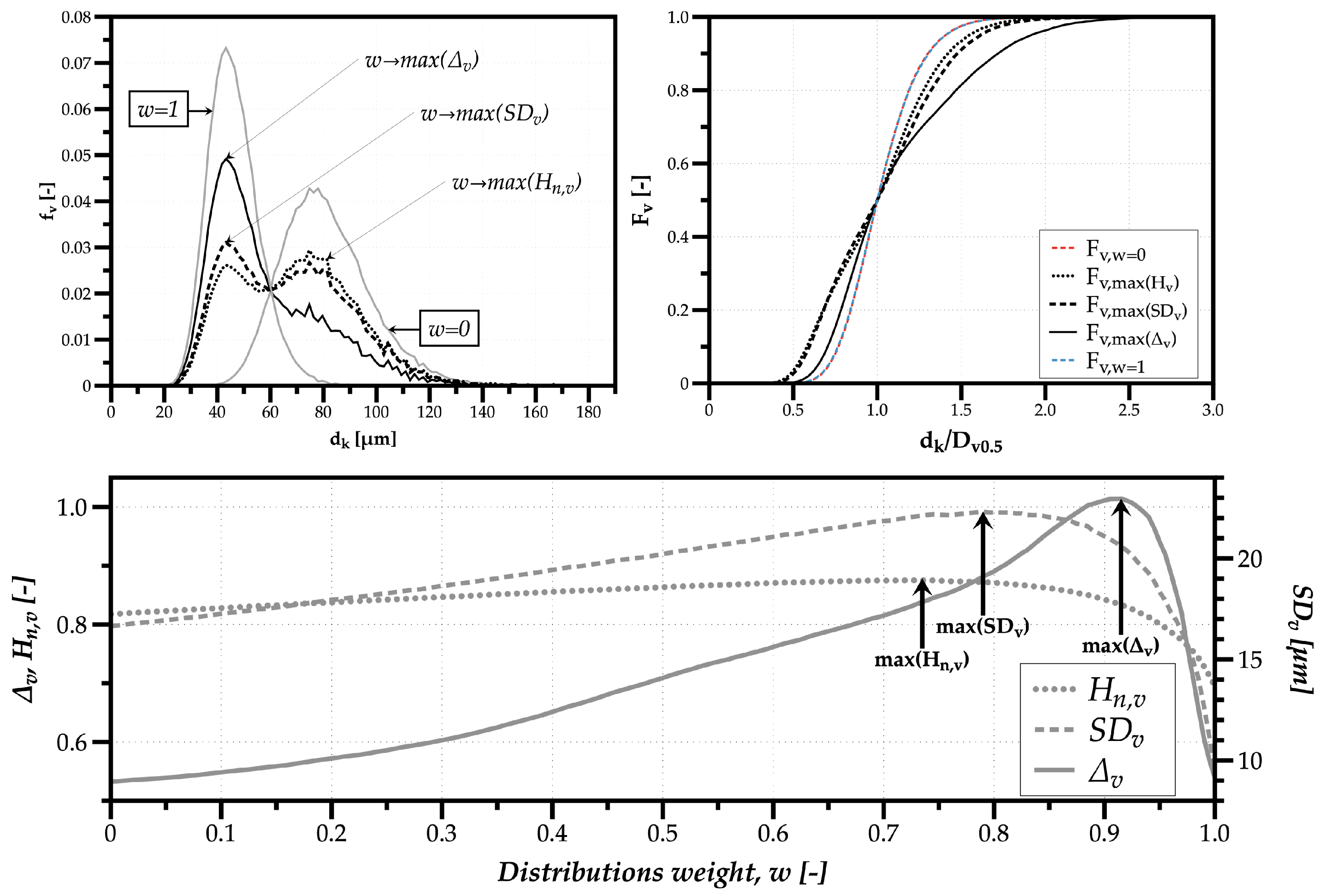
Considering a total sample of droplets, the simulated spray fixes the shape of both distributions mixed with , and uses distinct geometric mean diameters of m and 70 m to mix sprays around larger and smaller drop sizes. The weight corresponds to the Log-Normal distribution of m and to the distribution around smaller sizes. Figure 6 shows on the top left the volume-weighted drop size distributions simulated with w = 0, 1 and the distributions corresponding the the maximum values obtained for the normalized Shannon entropy (), volume-weighted standard deviation (), and relative span (). The number of classes used the Rice Rule (see Section 1). On the top right are the corresponding volume-based cumulative drop size distributions. Below is the comparison of all indicators for the Drop Size Diversity with the variation of the weight w attributed to each distribution.
The first observation concerns the results obtained for each distribution with w = 0 and w = 1. Since the Log-Normal shape parameter is the same for both distributions, the cumulative distributions are equal when classes are divided by , which is why one obtains equal values for the relative span .
The second observation are the implications of probability values for each isolated distribution for the normalized Shannon entropy and the volume-weighted standard deviation. Namely, the lower probability values for the distribution with larger diameters, indicates a higher number of relevant droplets in the spray relative to the distribution with smaller drop sizes, . Accordingly, the values for and are higher for w = 0 compared to w = 1.
The third and final observation concerns the distribution with the highest polydispersion degree obtained through the maximum value for , where the similarity of the two peak values of prove a balanced mixing between clusters of droplets from each of the original distributions, resulting in a spray with a larger polydispersion of drop sizes. Concerning the volume-weighted standard deviation, the distribution with the maximum heterogeneity degree is similar to the distribution with maximum polydispersion—however, with 5.5% more droplets around the distribution of smaller sizes since it produces a slight increase in the largest difference between the smallest and largest relevant size classes in the mixed spray. As to the relative span, due to a decrease of as droplets from the distribution with smaller sizes begin to constitute the larger part of spray liquid volume, the maximum reached only at has no apparent physical reason. In this sense, in this work, the advice is to gradually cease to use the relative spam as an indicator to characterize drop size diversity.
The following and final section applies the guidelines outlined above to the characterization of nanofluid sprays generated by a pressure-swirl atomizer.
3. Characterization of Nanofluid Sprays: An Example
The droplets in the nanofluid spray have multiple sizes and velocities. The measurement technique used is a 1D Phase-Doppler Interferometer (PDI), which is a single point laser diagnostic technique. Thus, the information provided has a mesh grid defined for the type of spray being characterized. In this case-study, the PDI measurement system retrieves information of radial profiles since the spray issued from a pressure-swirl atomizer is axisymmetric, considering two different measurement planes perpendicular to the spray penetration direction (Z) below the injector nozzle at Z =10 mm and Z = 20 mm. More details on the diagnostic technique can be found in Malỳ et al. [21]. The first step of every standard spray characterization is to report the mean quantities of size and velocity. Despite the loss of information relative to the size distributions, the quantitative data are useful for validation of numerical simulations in sprays. In addition, it is a picture of the global characteristics of the spray.
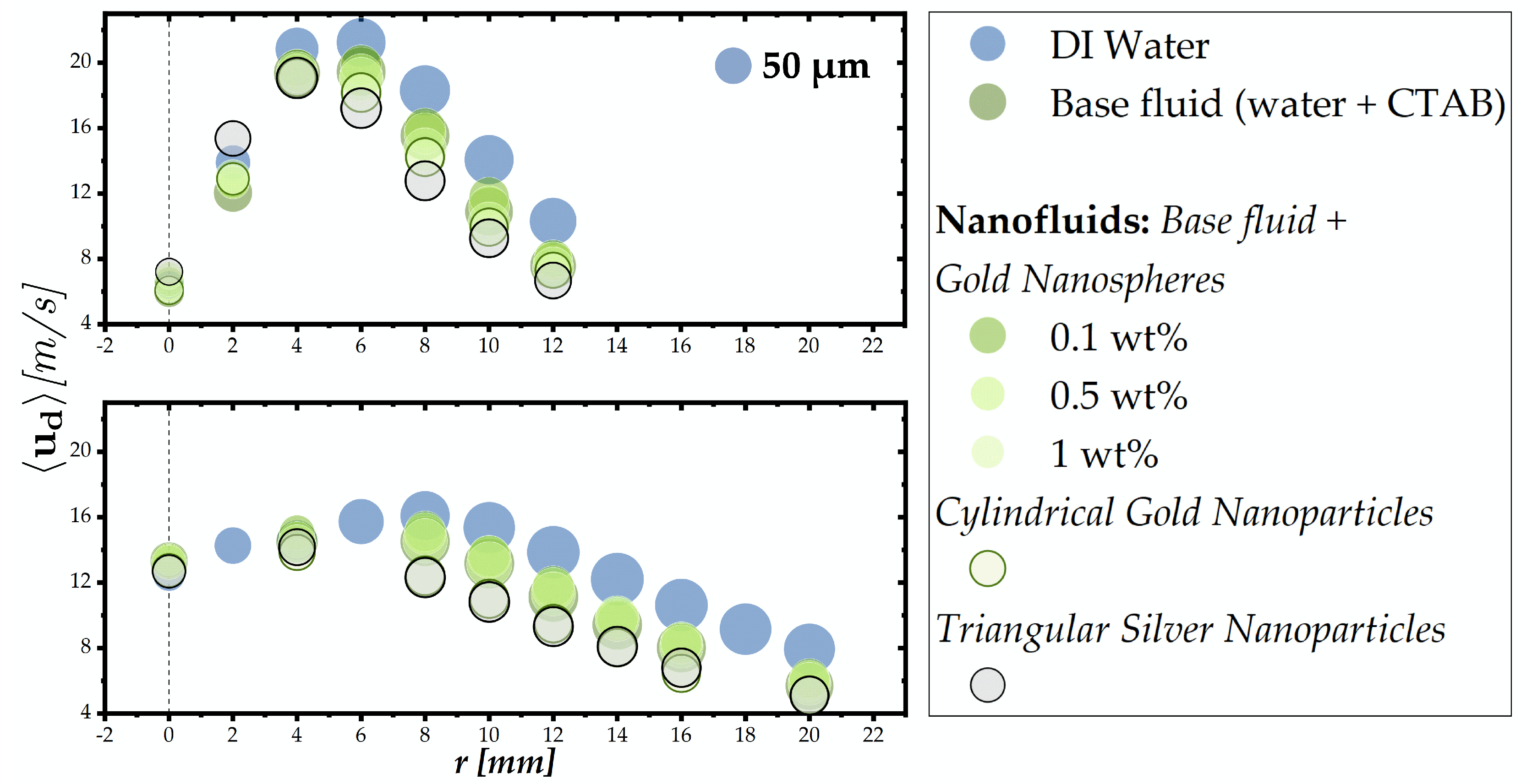
Figure 7 depicts the mean velocity of the droplets of the hollow cone spray structure for different working fluids and the size of symbols is proportional to drop size. These fluids are distilled water and a water based solution with a surfactant named CTAB-cetyltrimethylammonium bromide (water + 0.05 wg% CTAB). Different mettallic nanoparticles added to the base fluid are what forms the so-called nanofluids, i.e., liquid based suspensions of nanometer-sized particles (<100 nm). The surfactant is added to stabilize the suspension, precluding particles clustering and delaying their deposition. The purpose of nanofluids is to produce liquids with enhanced thermal properties, for example, a higher overall thermal conductivity for thermal management applications like spray cooling of high-power electronic devices. However, the addition of these nanoparticles may change the liquid’s thermophysical properties, i.e., the viscosity, thus, is likely to alter the atomization processes and the spray characteristics.
In this case, the mean diameter is , obtained from a volume-weighted drop size distribution because the application in mind is spray cooling. Therefore, any effect due to the size of droplets is related to the liquid volume of the spray impinging on a heated surface. As to the mean velocity, this is where the effects of adding a surfactant become noticeable.
The information given by the average velocities obtained for mm and mm mainly allows for identifying the region of the faster droplets, after which the variation remains similar regardless of the liquid used. Faster droplets are present in the region of the liquid sheet forming the cone, where the number of droplets is also higher. This is actually the region where one can see some differences between the various working fluids, particularly at mm, where the spray is fully developed in terms of breakup atomization mechanisms [21]. The main difference observed is due to the addition of the surfactant, which decreases the surface tension of the base fluid (water and surfactant) in comparison with water. This property affects the size of droplets and, consequently, how these interact with the surrounding environment, leading to changes in momentum transfer expressed by the variations of the mean velocity.
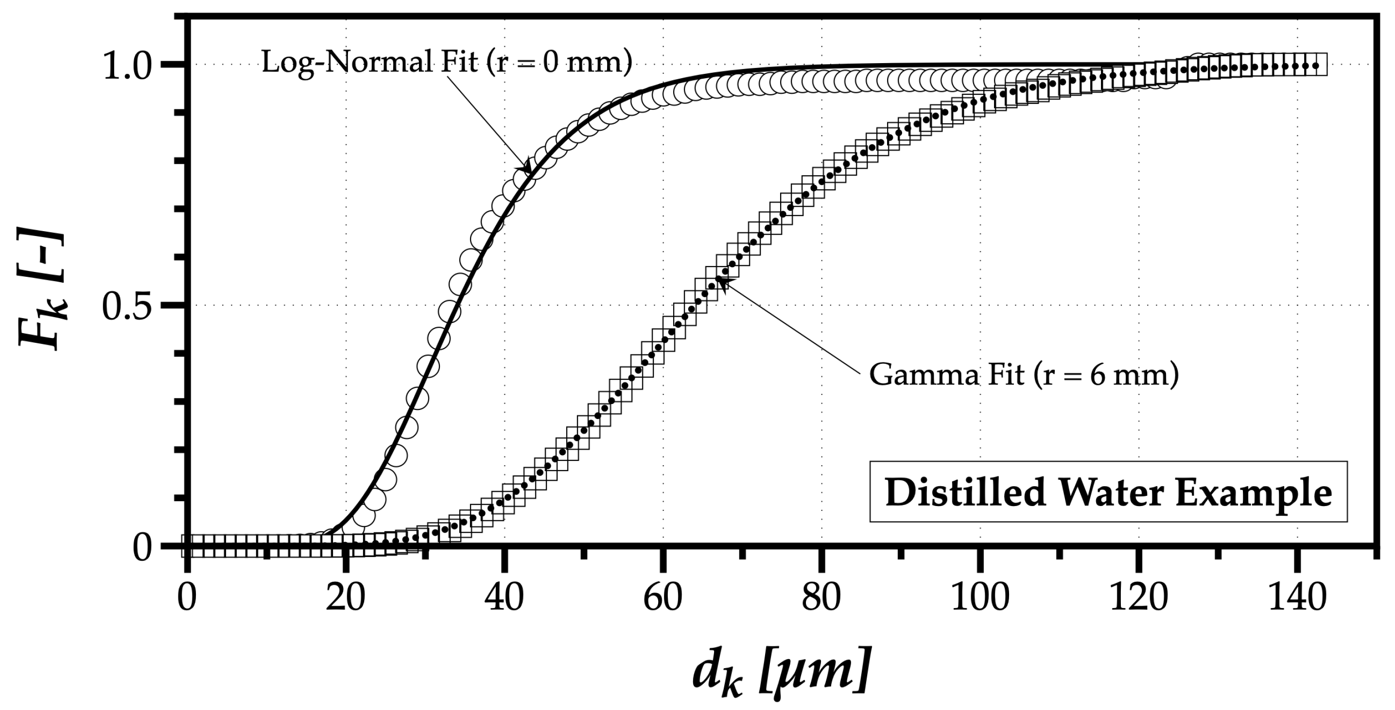
Despite their value, reporting mean quantities limits spray characterization. The presentation of the results should increase the informational value of data, and enable the reconstruction of the measured distributions compared to reporting its moments alone. Therefore, one could investigate if probability mathematical functions, such as the Log-Normal, Gamma, Weibull, and Nukiyama–Tanasawa can describe the histograms organizing the spray drop sizes by classes. Figure 8 shows examples for the distilled water spray in two radial locations, where the fitting functions that best described the probability of presence of droplets in the spray at r = 0 mm the Log-Normal—Equation (6)—and at r = 6 mm Gamma- Equation (7), probability distribution functions.
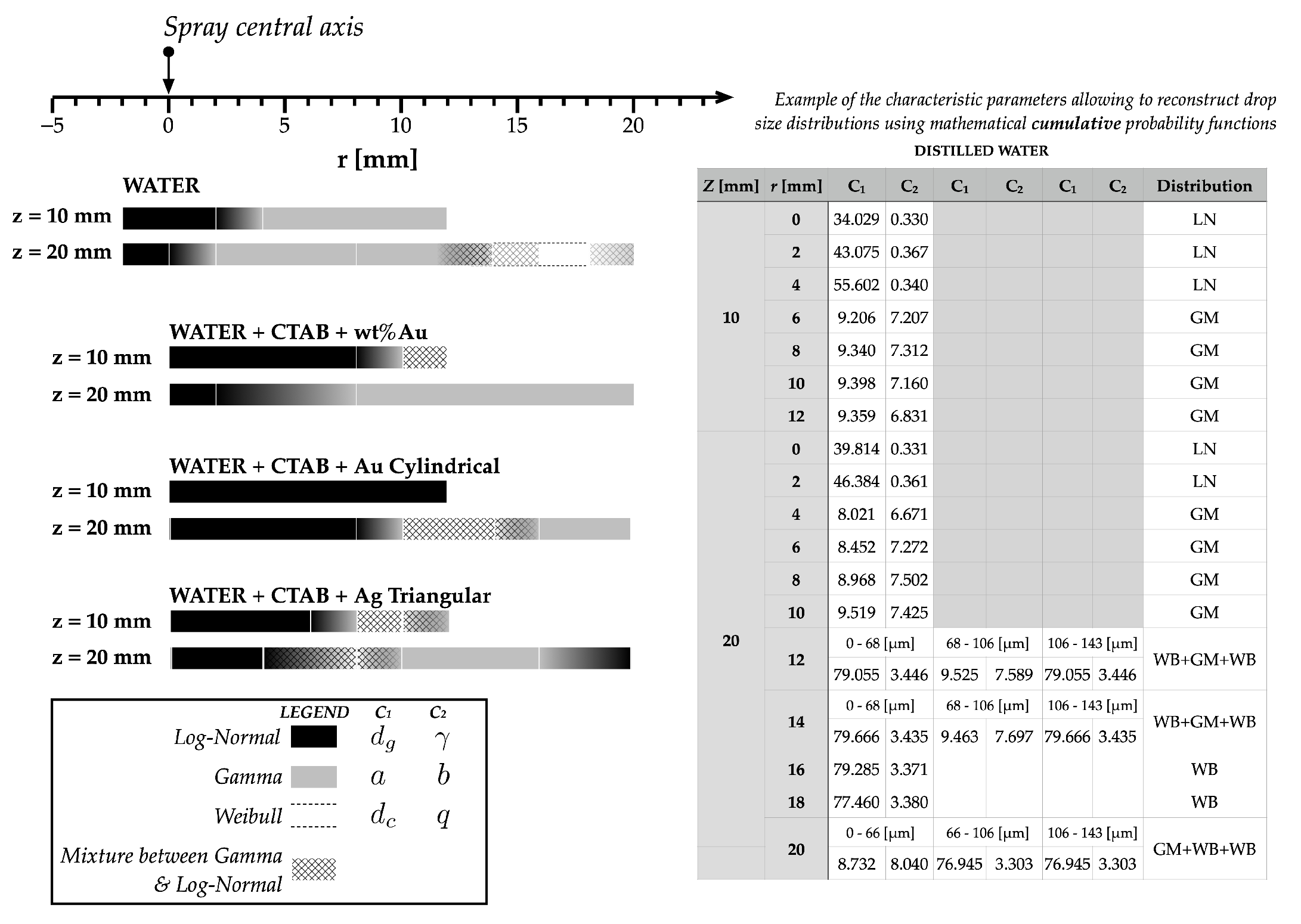
Using a Kolmogorov–Smirnov test to evaluate the best fitting, including combinations of probability distribution functions (pdf), Figure 9 maps the results for Z = 10 and 20 mm. On the right, it shows an example for distilled water of the pdf characteristics allowing the reconstruction of spray data at the measured locations, where and are the scale and shape parameters for each kind, also included in the legend. It is noteworthy that the Nukiyama–Tanasawa empirical distribution did not produce the best fitting in any measurement point, spray condition, or contribution to a mixed cumulative distribution function.
The spray analyzed is a hollow-cone, which means the formation of a liquid sheet at the nozzle exit further disintegrates into ligaments, and these fragment into droplets. In the central region, the momentum exchanges between smaller droplets and air leads to a dragging effect of these droplets into the central region of the spray, as expressed by the lower mean diameter shown in Figure 7. According to the interpretation delineated in Section 2.2, the Log-Normal predominance in the central region would be a expression of these transport phenomena, while in the regions of higher velocity, likely the result of spray formation through the fragmentation of ligaments, the gamma produces the best fitting. In the outer regions of the spray, the best fittings of the Weibull, in the case of Distilled water, and combination of pdfs indicate transition regions and, despite being unclear what is the physical meaning of these transitions, the identification of their location within the spray structure is a valuable insight. The final observation is the effect of the nanoparticles shape on the spray structure. While in the mean sizes, these differences were negligible, in dynamic terms, they were not.
The results in Figure 9 indicated as WATER + CTAB + wt% Au correspond to the spray of the base fluid and the base fluid plus different percentages of gold nanospheres (0.1, 0.5, 1 [wt%]), but the best pdf fitting map was the same, which means that gold nanospheres are not likely to alter the spray structure of the base fluid. However, gold cylindrical nanoparticles and silver triangular led to changes in the spray structure, and these results are coherent with the mean velocity values, but adds a substantial interpretative value.
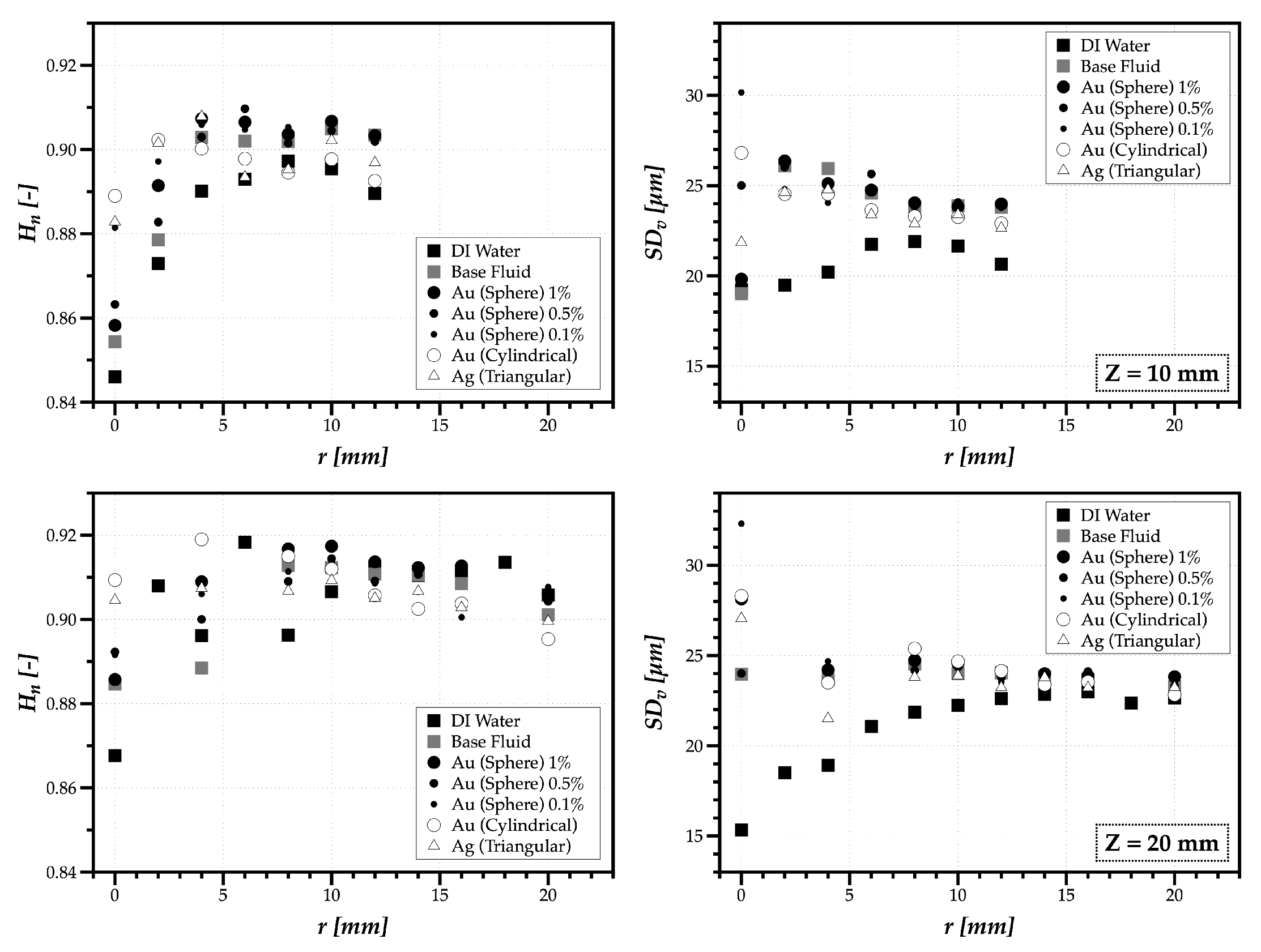
Finally, in this work, we introduced the concept of drop size diversity to better understand the many different sizes relevant in a spray, as well as how different the relevant sizes in a spray are. The polydispersion degree given by the normalized Shannon entropy, , and spray heterogeneity degree given by the volume-weighted standard deviation, [m], can describe this diversity, as depicted in Figure 10.
In the case of distilled water, the results show a higher polydispersion degree around mm, where the spray heterogeneity degree also becomes higher. However, despite local changes in , the behavior does not seem significantly affected by adding surfactant to produce the base fluid, and further adding nanoparticles. However, in terms of heterogeneity, the results are different. The addition of surfactant exerts a major effect on the heterogeneity of the spray characteristics. However, the addition of nanoparticles produces a negligibly effect. Consequently, one may also expect a minor effect of the nanoparticles during spray impact. This can actually be a beneficial feature, for instance, in spray cooling applications, as it suggests that the nanoparticles can be used to alter the thermal properties of the working fluids, without significantly affecting the main spray characteristics.
4. Conclusions
The characterization of a spray is not merely acquiring information on the size and velocity of its droplets in several locations from single-point measurement techniques, or in several planes from 2D- or 3D-measurement techniques. Although it is essential to acquire enough information, as explored here through an information theory approach, the clarity of the research question associated with the spray characterization is very much like the clarity in the display and analysis of data. Therefore, a well-defined research question is what guides the kind of spray characterization performed. In this article, we review the statistical language used in spray characterization, and:
- the differences between organizing spray data using probability histograms or histograms of probability density;
- how to choose the number of classes in histrograms;
- the different kinds of probability histograms considering the number of droplets, their area, or the liquid volume, and corresponding moments;
- a method based on the excess entropy from information theory to assess if there is enough information for post-processing;
- the physical meaning of fitting mathematical probability distribution functions, namely the Log-Normal, Gamma, and Weibull, to spray data;
- and introduce, for the first time, the notion of Drop Size Diversity with its polydispersion and heterogeneity degrees quantified by the normalized Shannon entropy and volume-weighted standard deviation, respectively.
Finally, the topics explored on spray characterization are applied to nanofluid sprays to explore the effect of introducing a surfactant and nanoparticles on the spray structure and dynamic characteristics.
Author Contributions
Conceptualization, investigation, M.O.P.; resources, A.S.M. and A.L.M.; writing–original draft preparation, M.O.P; writing–review and editing, M.O.P and A.S.M.; project administration, A.L.M.; funding acquisition, A.S.M. and A.L.M. All authors have read and agreed to the published version of the manuscript.
Funding
Ana S. Moita would like to acknowledge project No. 030171 funded by LISBOA-01-0145-FEDER- 030171/PTDC/EME-SIS/30171/2017, and project UTAP-EXPL/CTE/0064/2017.
Conflicts of Interest
The authors declare no conflict of interest.
Abbreviations
The following abbreviations are used in this manuscript:
| CTAB | CetylTrimethylAmmonium Bromide |
| DSD | Drop Size Diversity |
| PDI | Phase-Doppler Interferometer |
References
- Sturges, H.A. The choice of a class interval. J. Am. Stat. Assoc. 1926, 21, 65–66. [Google Scholar] [CrossRef]
- Doane, D.P. Aesthetic frequency classifications. Am. Stat. 1976, 30, 181–183. [Google Scholar]
- Hyndman, R.J. The Problem with Sturges Rule for Constructing Histograms; Monash University: Melbourne, Australia, 1995. [Google Scholar]
- Scott, D.W. On optimal and data-based histograms. Biometrika 1979, 66, 605–610. [Google Scholar] [CrossRef]
- Freedman, D.; Diaconis, P. On the histogram as a density estimator: L2 theory. Z. Wahrscheinlichkeit 1981, 57, 453–476. [Google Scholar] [CrossRef] [Green Version]
- Terrell, G.R.; Scott, D.W. Oversmoothed nonparametric density estimates. J. Am. Stat. Assoc. 1985, 80, 209–214. [Google Scholar] [CrossRef]
- Panão, M.; Moreira, A. A real-time assessment of measurement uncertainty in the experimental characterization of sprays. Meas. Sci. Technol. 2008, 19, 095402. [Google Scholar] [CrossRef]
- Sowa, W. Interpreting mean drop diameters using distribution moments. At. Sprays 1992, 2, 1–15. [Google Scholar] [CrossRef]
- Panão, M.R.; Radu, L. Advanced statistics to improve the physical interpretation of atomization processes. Int. J. Heat Fluid Flow 2013, 40, 151–164. [Google Scholar] [CrossRef]
- Panão, M.R.O. Assessment of measurement efficiency in laser-and phase-Doppler techniques: An information theory approach. Meas. Sci. Technol. 2012, 23, 125304. [Google Scholar] [CrossRef]
- Feldman, D.P.; McTague, C.S.; Crutchfield, J.P. The organization of intrinsic computation: Complexity-entropy diagrams and the diversity of natural information processing. Chaos: Interdiscip. J. Nonlinear Sci. 2008, 18, 043106. [Google Scholar] [CrossRef] [PubMed]
- Naruemon, I.; Liu, L.; Liu, D.; Ma, X.; Nishida, K. An Analysis on the Effects of the Fuel Injection Rate Shape of the Diesel Spray Mixing Process Using a Numerical Simulation. Appl. Sci. 2020, 10, 4983. [Google Scholar] [CrossRef]
- Archambault, M.R. A discussion on the stochastic modeling of spray flows. At. Sprays 2009, 19, 1171–1191. [Google Scholar] [CrossRef]
- Déchelette, A.; Babinsky, E.; Sojka, P. Drop size distributions. In Handbook of Atomization and Sprays; Springer: Berlin, Germany, 2011; pp. 479–495. [Google Scholar]
- Lefebvre, A.H.; McDonell, V.G. Atomization and Sprays; CRC Press: Boca Raton, FL, USA, 2017. [Google Scholar]
- Villermaux, E.; Marmottant, P.; Duplat, J. Ligament-mediated spray formation. Phys. Rev. Lett. 2004, 92, 074501. [Google Scholar] [CrossRef] [PubMed] [Green Version]
- Villermaux, E. Fragmentation. Annu. Rev. Fluid Mech. 2007, 39, 419–446. [Google Scholar] [CrossRef]
- Li, X.; Tankin, R.S. Droplet size distribution: A derivation of a Nukiyama-Tanasawa type distribution function. Combust. Sci. Technol. 1987, 56, 65–76. [Google Scholar]
- Panão, M.R.O. Redefining spray uniformity through an information theory approach. At. Sprays 2016, 26, 1069–1081. [Google Scholar] [CrossRef]
- García, J.; Lozano, A.; Alconchel, J.; Calvo, E.; Barreras, F.; Santolaya, J. Atomization of glycerin with a twin-fluid swirl nozzle. Int. J. Multiph. Flow 2017, 92, 150–160. [Google Scholar] [CrossRef]
- Malỳ, M.; Moita, A.; Jedelsky, J.; Ribeiro, A.; Moreira, A. Effect of nanoparticles concentration on the characteristics of nanofluid sprays for cooling applications. J. Therm. Anal. Calorim. 2019, 135, 3375–3386. [Google Scholar] [CrossRef] [Green Version]
Figure 1.
Example of the effect of changing the bin size in discrete probability (a) and probability density (b) size distributions. The simulated data follow a lognormal distribution function.
Figure 1.
Example of the effect of changing the bin size in discrete probability (a) and probability density (b) size distributions. The simulated data follow a lognormal distribution function.

Figure 2.
Example of the effect of changing the number of classes in details obtained on the probability density distribution of a mixture between two clusters described by distinct lognormal distributions, considering different sample sizes of (a) N = 10 and (b) N = 10 droplets.
Figure 2.
Example of the effect of changing the number of classes in details obtained on the probability density distribution of a mixture between two clusters described by distinct lognormal distributions, considering different sample sizes of (a) N = 10 and (b) N = 10 droplets.

Figure 3.
Variation of three Drop Size Diversity Indicators, the Relative Span (), the normalized Shannon Entropy (), and the volume-weighted standard deviation () for the mixing of two monosize droplet clusters.
Figure 3.
Variation of three Drop Size Diversity Indicators, the Relative Span (), the normalized Shannon Entropy (), and the volume-weighted standard deviation () for the mixing of two monosize droplet clusters.

Figure 4.
Variation of the numerator difference of the relative span (D–D), and the 50% spray liquid volume representative diameter (), with the weight parameter w.
Figure 4.
Variation of the numerator difference of the relative span (D–D), and the 50% spray liquid volume representative diameter (), with the weight parameter w.

Figure 5.
Variation of three Drop Size Diversity Indicators, the Relative Span (), the normalized Shannon Entropy (), and the volume-weighted standard deviation () for the mixing of two monosize droplet clusters, and the corresponding distributions for the maximum value obtained by each indicator.
Figure 5.
Variation of three Drop Size Diversity Indicators, the Relative Span (), the normalized Shannon Entropy (), and the volume-weighted standard deviation () for the mixing of two monosize droplet clusters, and the corresponding distributions for the maximum value obtained by each indicator.

Figure 6.
Results for the volume-weighted Log-Normal mixed spray, corresponding cumulative drop size distributions for w = 0, 1, and the values corresponding the maximum (w = 0.735), (w = 0.790) and (w = 0.915). Below is the variation of , , and with the weight parameter w.
Figure 6.
Results for the volume-weighted Log-Normal mixed spray, corresponding cumulative drop size distributions for w = 0, 1, and the values corresponding the maximum (w = 0.735), (w = 0.790) and (w = 0.915). Below is the variation of , , and with the weight parameter w.

Figure 7.
Mean velocity, [m/s] of the spray droplets for mm (top) and mm (bottom).

Figure 8.
Example of the results of the cumulative curve fitting for Distilled water, r = 0 mm where the best fitting occurred with a Log-Normal, Equation (6), and r = 6 mm with a best fitting through a Gamma function, Equation (7).

Figure 9.
Radial profiles of the mathematical probability functions that best fitted the experimental results for all experimental conditions and measurement planes considered. The table on the right exemplifies the data that allows the reconstruction of each cumulative distribution. Some included more than one function in different drop size ranges.

Figure 10.
Polydispersion degree given by the normalized Shannon entropy, , and spray heterogeneity degree given by the volume-weighted standard deviation, [ m], for the planes of mm (top) and mm (bottom).
Figure 10.
Polydispersion degree given by the normalized Shannon entropy, , and spray heterogeneity degree given by the volume-weighted standard deviation, [ m], for the planes of mm (top) and mm (bottom).

© 2020 by the authors. Licensee MDPI, Basel, Switzerland. This article is an open access article distributed under the terms and conditions of the Creative Commons Attribution (CC BY) license (http://creativecommons.org/licenses/by/4.0/).
Share and Cite
MDPI and ACS Style
Panão, M.O.; Moita, A.S.; Moreira, A.L. On the Statistical Characterization of Sprays. Appl. Sci. 2020, 10, 6122. https://0-doi-org.brum.beds.ac.uk/10.3390/app10176122
AMA Style
Panão MO, Moita AS, Moreira AL. On the Statistical Characterization of Sprays. Applied Sciences. 2020; 10(17):6122. https://0-doi-org.brum.beds.ac.uk/10.3390/app10176122
Chicago/Turabian StylePanão, Miguel O., Ana S. Moita, and António L. Moreira. 2020. "On the Statistical Characterization of Sprays" Applied Sciences 10, no. 17: 6122. https://0-doi-org.brum.beds.ac.uk/10.3390/app10176122
Note that from the first issue of 2016, this journal uses article numbers instead of page numbers. See further details here.