Single-Shot Object Detection with Split and Combine Blocks


1
Tianjin Key Laboratory for Control Theory and Applications in Complicated Systems, Tianjin University of Technology, Tianjin 300384, China
2
Intelligent Manufacturing College, Tianjin Sino-German University of Applied Sciences, Tianjin 300350, China
*
Authors to whom correspondence should be addressed.
†
These authors contributed equally to this work.
Appl. Sci. 2020, 10(18), 6382; https://0-doi-org.brum.beds.ac.uk/10.3390/app10186382
Submission received: 2 August 2020
/
Revised: 2 September 2020
/
Accepted: 10 September 2020
/
Published: 13 September 2020
(This article belongs to the Special Issue Deep Learning Applied to Image Processing)
Abstract
:Feature fusion is widely used in various neural network-based visual recognition tasks, such as object detection, to enhance the quality of feature representation. It is common practice for both the one-stage object detectors and the two-stage object detectors to implement feature fusion in feature pyramid networks (FPN) to enhance the capacity to detect objects of different scales. In this work, we propose a novel and efficient feature fusion unit, which is referred to as the Split and Combine (SC) Block, that splits the input feature maps into several parts, then processes these sub-feature maps with different emphasis, and finally gradually concatenates the outputs one-by-one. The SC block implicitly encourages the network to focus on features that are more important to the task, thus improving network efficiency and reducing inference computations. In order to prove our analysis and conclusions, a backbone network and an FPN employing this technique are assembled into a one-stage detector and evaluated on the MS COCO dataset. With the newly introduced SC block and other novel training tricks, our detector achieves a good speed-accuracy trade-off on COCO test-dev set, with 37.1% AP (average precision) at 51 FPS and 38.9% AP at 40 FPS.
1. Introduction
Detecting objects from given images or videos is a fundamental but crucial research area in computer vision. Due to the excellent performance of feature extraction and representation learning, convolutional neural networks (CNNs) have become an important driver in promoting object detection progress [1]. With the emergence of large open source datasets and the availability of computation resources, CNNs-based object detectors flourish and can generally fall into two categories: one-stage approaches and two-stage approaches. Attributed to the higher computational efficiency and lower inference latency, one-stage detectors have gradually received more attention in real-time applications [2].
Scaling up CNNs by their depth, width or input image resolution is the most common and effective way to obtain better accuracy [3]. However, the ever-increasing trainable parameters, nonlinear activation units, and receptive fields cause difficulty with training and optimization. In order to overcome these obstacles, more effort is directed into devising connect patterns between different layers and modules to make the network efficient. In practice, many of the latest network structures emphasize the value of short paths from shallower layers to deeper layers. ResNet [4] proves the significance of skip connections for training deep networks in classification and localization tasks, and facilitates a dramatic variety of deep architectures. Dense convolutional network (DenseNet) [5] maximizes the feature transmission between different layers to improve parameter efficiency and reduce training difficulty. The input feature information of each layer in DenseNet is composed of the output of all preceding layers. Deep layer aggregation (DLA) [6] aggregates the feature hierarchy in a deeper method. DLA fuses feature information across various depths, scales, and resolutions to promote network performance, parameter efficiency, and reduce memory usage. Hourglass [7] processes input signals through repeated bottom-up, top-down inference paths, and then captures and merges information across all scales in this process. The excellent performance of these models indicates that feature fusion plays a central role in network performance.
It is common practice to employ a feature pyramid to assist algorithms in capturing objects of a wide range of scales. Assign different priorities based on scales of object instances. High-level, low-resolution feature maps are generally responsible for large targets, while low-level, high-resolution feature maps are generally responsible for small targets. Due to the expensive computing and storage costs, recent studies desert the image pyramid, and instead exploit the inherent pyramid hierarchy formed in forward propagation to construct feature pyramids. The feature pyramid network (FPN) [8] introduces the lateral connections to integrate bottom-up pathways with top-down pathways. This architecture combines shallower, spatially strong features with deeper, semantically strong features, and ultimately enriches semantics for each feature maps. Adaptively spatial feature fusion (ASFF) [9] learns the weights of feature maps at all levels during propagation, and then aggregates feature maps of different scales based on these weights. ASFF suppresses inconsistency between different feature maps with marginal computing cost. A multi-level feature pyramid network (MLFPN) [10] first fuses feature maps at all levels, then extracts and concatenates multi-depth feature maps of the equivalent scales, and finally utilizes Squeeze-and-Excitation networks (SENets) [11] to recalibrate the importance of each channel. These advanced feature pyramid variants deliver excellent performance gain, and do not demand much extra inference overhead, which demonstrates that good feature fusion strategies are the key to reach their full potential in visual tasks.
In this work, we construct a novel and valid unit to implement better feature fusion, and ultimately improve the quality of feature representation, designated as a Split and Combine (SC) block. The SC block evenly splits the input feature information into several parts and processes them in parallel by branches with different depths, and then implements the feature fusion between these branches. This mechanism guides the network to process feature information with different emphasis, and then continuously transmit the information that is more critical to the task to the subsequent layers. The structure of a SC block can be seen in Figure 1. We employ the conv block (e.g., a convolution, a normalization, and a nonlinear activation) and identity mapping to process information. First of all, a conv module maps the input to the feature maps , where the channel dimension is reduced to depress computational demand. The feature maps and then goes through a split operation, which equally divides the feature maps into w parts across their channel dimension. These sub-feature maps with spatial dimensions of are then transmitted to network branches, and the output of each branch is passed to the next branch, from a shallower one to a deeper one. Finally, concatenate the output of the last branch with the feature maps to further promote feature fusion. The purpose of this architecture is to direct the network to assign an appropriate number of learnable parameters to each part of the feature information based on its contribution to the final task, thus allowing the network to focus on the more critical features and improve the quality of feature representation.
The architecture of our SC block is simple, clear, and extendable. Block variants can be easily obtained by modifying the number and depth of branches within the SC block. Performance can be further improved by assembling the proposed SC block with other existing excellent architectures, such as ResNet, DenseNet, and Deformable ConvNets [12,13]. The SC block does not use any bells and whistles and causes only a slight increase in network complexity and inference latency. To verify the effectivity of the proposed block, we utilize SC blocks to build a backbone network and an FPN, and design a one-stage detector based on them. Our detector is evaluated on a highly competitive MS COCO [14] dataset and exhibits good detection accuracy while maintaining high detection speed. The best model achieves an AP of 38.9% with 40 FPS on a COCO test-dev set.
2. Related Work
2.1. Two-Stage Object Detectors
Two-stage detectors have dominated the CNNs-based object detection algorithms. These region-based approaches primarily represent the frameworks as two stages: generating category-independent potential object proposals, and then classifying each candidate proposals into given categories or background. RCNN [15] acquires region proposals via selective search and then dispatches these potential areas to a pretrained convolutional network for fine-tuning. Fast RCNN [16] simultaneously implements object category prediction and bounding box regression, and transports the original image to the convolutional network for feature extraction. In Faster RCNN [17], a more efficient and more accurate subnetwork, called the Region Proposal Network (RPN), is exploited in place of selective search to produce region proposals, which enables the detector to be present in a fully convolutional fashion. Numerous variants have emerged, such as [18,19,20]. As a common processing step for detectors, generating region proposals is intuitive, efficient, and far-reaching.
2.2. One-Stage Object Detectors
One-stage approaches do not include region proposal generation and complete all calculations through one network. OverFeat [21] is one of the first completely CNNs-based one-stage detectors, which is of great importance for subsequent research. YOLO-v1 [22] divides the input image into S × S grids, and then directly regresses the coordinates, categories, and confidence of the bounding boxes from each grid. YOLOv2 [23] proposes Darknet-19 as the backbone, adds batch normalization layers, uses multi-scale training strategy, and adjusts k-means to obtain anchor boxes. YOLO-v3 [24] replaces Darknet-19 with Darknet-53 to strengthen the capacity of feature extraction, and employs three feature maps of different spatial resolutions to capture objects with various scales. SSD (Single shot detector) [25] predicts objects through several feature maps of different depths in the network, each of which is responsible for the prediction of appropriate size bounding boxes. In general, one-stage detectors trail two-stage ones in the precision but are faster, simpler, and less dependent on the storage space and computing power of the device.
2.3. Objects as Points
Faster RCNN first densely distributes anchor boxes over the feature maps to improve multi-scale prediction capabilities. These pre-defined boxes, with various scales and aspect ratios, serve as references to predict location. After noticing the impressive performance improvements caused by anchor boxes, this mechanism gradually becomes the necessary component both in numerous two-stage and one-stage detectors. Recently, owing to the constant improvement of the network property and the emergence of special loss functions [26,27], anchor-free detectors stand out again. It is common to implement anchor-free detection by keypoints or centerpoints estimation [28]. Law et al. [29] present an object instance by estimating its top-left corner and bottom-right corner. In addition, they also improve the accuracy of corner location through a corner pooling layer. Zhou et al. [30] represent an object instance by estimating the top, bottom, left, and right extreme points and one center point. Then, determine whether these extreme points belong to the same object based on geometric information. Based on the previous approach of detecting the top-left and the bottom-right points, Duan et al [31] add a center point detection procedure to further improve performance. In addition, they introduce cascade corner pooling and center pooling to assist in the precise localization of these points. Zhou et al. [32] determine a bounding box by directly predicting the center point and other properties of the object, such as the width and height—simple but effective. These keypoint-based anchor-free detectors are end-to-end trainable, simple, fast, and efficient.
3. Method
3.1. Split and Combine Block
A split-and-combine block is a unit for enhancing feature fusion that can be directly integrated directly into other architectures by inserting it after the nonlinear activation layers. We expect to improve the quality of output feature maps by ranking the feature information according to its importance. There is no down-sampling or up-sampling operation in the SC block, and the feature maps have a constant resolution. As illustrated in Figure 1, first, the input feature maps pass through a non-linear transformation to modify the dimensions, and new feature maps is obtained. We only compress the channel dimension to reduce computation load. For model efficiency, we simplify the structure of , which is composed of a convolutional layer, a normalization layer, and a nonlinear activation layer. In the split procedure that follows, we split into w parts, described as , which have the same spatial dimension of . These sub-feature maps are sent to multiple sampling branches with different numbers of . The first branch receives and processes sub-feature maps , so the output is obtained. Concatenate the with the feature maps of the same sampling depth in the second branch to perform feature fusion. The output of the second branch is obtained. Repeat the procedure until we obtain the output of the last branch . Subsequently, the number of channels of the feature maps and is compressed to half, and concatenate the results together to further promote feature fusion. Finally, the channel dimension of the feature maps is restored to the initial state, and the output is obtained. We can write a SC block as , where w refers to the number of branches within the block, and denote the number of on each branch. The output of each branch is referred as :
Here, the subscripts of represent multiple transformation operations, ⨁ indicates the feature concatenation. Consequently, the output feature maps of a SC block can be expressed as follows:
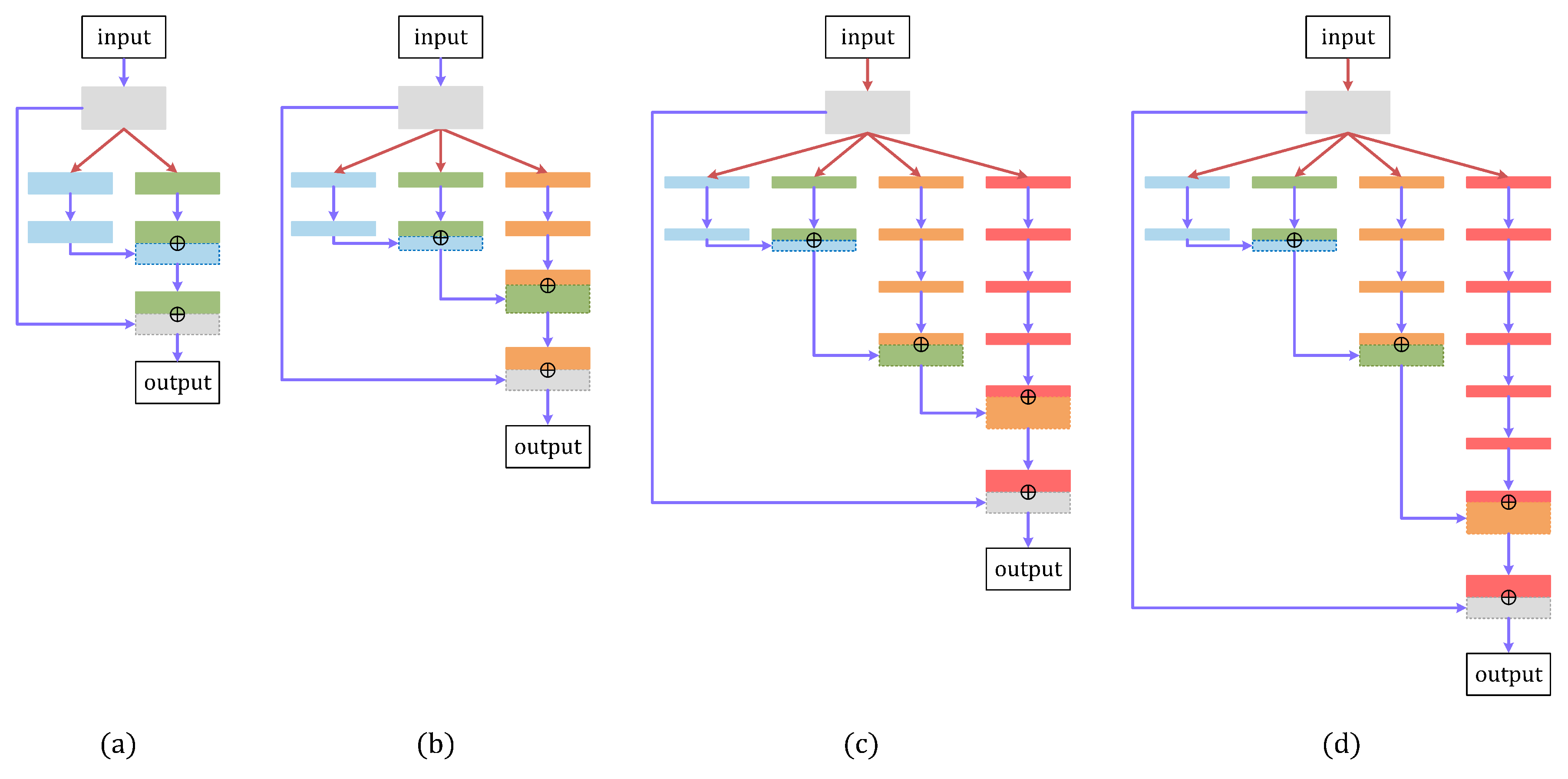
We stack SC variants together to constitute a deeper and larger network which can be applied to complex vision tasks. Ideally, as the network continues to learn, it gradually focuses the attention on more critical feature information so that the network can accomplish the task at a lower computational cost. It is worth noting that the input of each SC block is made up of the outputs of previous multiple layers. This structure shortens the gradient transmission path, facilitating the information flow and gradients’ propagation. Furthermore, it does not use the gradient information of the latter layer to update the weights of too many previous layers, avoiding network redundancy. We construct a backbone and an FPN based on several SC block variants in the next section. The diagram of these variants is shown in Figure 2.
3.2. Backbone and FPN
A similar structure to other methods, our detector is mainly composed of a backbone, an FPN, and a head [33]. They are applied separately to gather information from the input image, fuse feature maps at different depths to tackle the challenge of scale variation, and generate dense predictions of coordinates, scales, and categories of bounding boxes. We alternately stack multiple residual blocks and SC blocks to build the backbone network. A network is shown in Figure 3. All of the residual block herein is composed of a 3 × 3 convolutional layer, a normalization layer, and a skip connection layer followed by a nonlinear activation layer. The down-sampling operation in our experiments relies on the residual block with stride 2. As a result, five down-sampling is conducted in the backbone. The dimension setting of the feature maps refers to the previous network structure; we only use 1 × 1 or 3 × 3 filters to process the feature information.
We exploit the SC block to realize the multi-scale feature fusion, and propose a feature pyramid network SC-FPN; the diagram is illustrated in Figure 4. First, we choose feature maps at level 3 to 5 from the backbone to formulate the typical top-down FPN. indicate the newly generated feature maps. Then, an additional bottom-up pathway is connected behind the FPN to further boost the flow of information. We use the SC block to remodel and enlarge the PANet [34], as can be seen in Figure 5b. Feature maps are obtained. These feature maps with different spatial resolutions are then fused. A common solution is to adjust the dimension and then merge them together by element-wise sum or concatenation. Recent works point out the defect of integrating different resolution feature maps at the same proportion [35]. These feature maps of different resolutions contribute unequally to the detection of objects of varying sizes. To alleviate this issue, we exploit the SC block to merge multi-scale feature maps. As shown in Figure 5c, the feature maps are fed to an SC-fusion block to generate newly feature maps . In general, the low-resolution feature maps are more important to detect large objects. Therefore, we assign different levels of attention to these feature maps based on their spatial resolution, occupies first place, comes second and is the last. The SC-fusion block takes the as input, and merges the semantic information of and one by one. Sampling depth reflects the level of attention. We employ max pooling layers and the nearest neighbor method to eliminate dimension conflicts in the feature fusion process. denote the feature maps generated by SC-fusion blocks that are intended for final prediction.
3.3. Dense Predictions
We use feature maps with downsampling strides of 8, 16, and 32 compared to the input to predict the bounding box. The method of bounding box regression draws on a variety of novel ideas from recent works. For each level, the network finally outputs feature maps . The input image is divided into H × W grids; one grid is responsible for one object. Evaluated on an COCO dataset, we set including four offsets , , , , and 80 object categories. The highest category score of each prediction bounding box is used to represent the confidence, thus simplifying the calculation. For each bounding box, the center point coordinate, width, and height are as follows:
The center coordinate is limited at a certain grid by function , donates the coordinate of the upper left corner of the grid, the w, h are the width and height of anchor box which is generated by guided anchoring mechanism [36]. During training and test, we assign an anchor box to each grid. For instance, if input resolution is 416 × 416, the number of proposal is 416/32 × 416/32 + 416/16 × 416/16 + 416/8 × 416/8 = 3549.
We extract the center point coordinates of the ground truth onto feature maps and refer the ground truth centers as positive locations, and all others are negative. However, such a simple distinction mechanism can cause a huge imbalance between positive and negative samples, which has an adverse effect on network training. Therefore, we attempt to alleviate this problem by redefining positive and negative samples during training [37]. As shown in Figure 6, the locations close to the ground truth center can still generate high-quality bounding boxes, and we think these boxes can also contribute to the network leaning. A fraction of negative locations are defined as candidate locations, and the boundary boxes generated by these positions incorporate the calculation of the gradient. These candidate locations are near the positive locations, and theoretically can generate a high-quality bounding box which has at least 0.7 intersection over union (IoU) with the ground truth box. For each object, the maximum distance between candidate location and ground truth center is indicated by r, which is closely related to ground truth size. A set of cosine decay confidences are assigned to these candidate locations:
where the d is the distance between candidate locations and ground truth center. These confidences are placed on feature maps Y, and take the maximum in the overlapping part of adjacent candidate locations with the same class, if overlaps occur. The category loss function is as follows:
where and are hyper-parameters of the focal loss, is category prediction of feature maps , and the attracts more attention from the network on hard examples. The offsets , are trained with a binary cross entropy loss function, and , are trained with an loss. Furthermore, a Generalized Intersection over Union (GIoU) [38] loss function is exploited to better optimize the regression of bounding box, especially in the extreme case of no overlap. Aggregate all parts to form the overall training objective.
3.4. Training and Testing
Our detector SCNet is built on a Pytorch v1.5.1 framework with CUDA 10.2 and cuDNN v8.0.1. Adaptive Moment Estimation (Adam) [39] with the default setting is exploited to optimize the entire network. A learning rate is initialized with which increases in the first five warmup epochs from to , and then is reduced by a smoother cosine learning rate adjustment from to [40,41]. The detector is trained on two 2080ti GPUs with total batch size of 24 for 300 epochs. All the convolutional layers are initialized with an He weight initialization method [42], and the backbone is first fine-tuned at the 608 × 608 resolution for 50 epochs on the ImageNet dataset [43] to speed up the convergence. We use a convolutional layer, Cross mini-Batch Normalization (CmBN) [44], and Mish [45] activation to construct a conv block. Use the multi-scale training method to boost the robustness of the model. More specifically, after each iteration, the training resolution is randomly picked in with the aspect ratio as 1. We design a new data augmentation pattern called Admix which mixes five different images at a time; by comparison, CutMix [46] mixes two images and Mosaic mixes four images. Some examples of Admix are shown in Figure 7. We combine the Admix with several usual methods of data augmentation in training to alleviate the problem of overfitting and improve the generalization ability of the network, such as random horizontal flipping, random scaling, random cropping, random shifting RGB and random changing hue, saturation, and value. Undersized bounding box annotations (area < 8) are also filtered out after cropping. We use DropBlock [47] as the regularization technique and increase the block size at 90, 120, and 150 epochs, respectively. SPP [48] is integrated into our SC-PANet to further improve the discriminability and robustness of features. During inference, soft non-maximum suppression (Soft-NMS) [49] is used to filter out suboptimal predictions.
4. Experiments
SCNet is evaluated on the MS COCO dataset, which is a large-scale image dataset with abundant bounding boxes, segmentation, keypoints, and captioning annotations. Following the common practice, we use a 118k train set for training the detector, a 5k validation set for ablation studies, and a 20k test-dev set for measuring the final performance of our detector and comparing with other approaches. In all the experiments, we choose COCO-style detection metrics and mean Average Precision (mAP) to measure the performance. Evaluate the average precision over different IOU threshold, including 0.5 (), 0.75 (), and 10 values of 0.50: 0.05: 0.95 (AP). In addition, calculate the average precision for objects of different scales, including , , for small, medium, large objects (area < , < area < , < area), respectively.
4.1. Ablation Study
We adopted a variety of recent training tricks to improve the performance of SCNet. The ablation study begins with a baseline network which uses Batch Normalization layer [50], Relu activation, and decays the learning rate every 30 epochs. The baseline network is trained with the fixed input resolution of 608 × 608 and directly predicts the size of the bounding box with the exponential function. Herein, we evaluate the impetus of these elements, including CmBN, Mish, Admix, cosine, and warmup learning rate schedule, multi-scale training, DropBlock and SPP, to the final detection performance. SC-59 is chosen as the backbone network. The results can be found in Table 1, which are measured at 608 × 608 input resolution. Shorten training cycle time and save computation costs by transfer learning. All of the mentioned design decisions generate decent accuracy growth, and our detector achieves an AP of 38.8% on COCO val split after using these techniques in the training process. CmBN enhances the quality of statistics in the case of small batch sizes. Admix accumulates information from five different images, and, thanks to them, we complete the training of detectors on two GPUs. The learning rate scheduler, data augmentation, multi-scale training strategy, and Mish activation do not any add additional parameters, and there is almost no increase in inference time after usage. At each level, GA increases only two convolution layers; SPP introduces three max pooling layers and one concatenation operation, and the improvements are minimal in cost. DropBlock quits work during inference, and no additional computation is added. Our detector reaches 40 FPS on RTX 2080ti GPU.
The backbone SC-59 is then replaced with SC-47 and SC-32 networks to achieve different trade-offs in speed-accuracy. There is a similar structure to these backbone networks, with Figure 3 for reference. We employ SC-[2,1,2], SC-[3,1,1,2], SC-[3,2,2,4], SC-[4,2,2,4,6], SC-[3,2,2,4] blocks and residual blocks to construct SC-47 network, and use SC-[2,1,2], SC-[3,1,1,2], SC-[3,2,2,4], SC-[3,1,1,2], SC-[2,1,2] blocks and residual blocks to construct the SC-32 network. The evaluation results on the COCO val split are illustrated in Table 2. SCNet is tested on the same machine and uses all verified tricks in the training process. SCNet achieves a good speed-accuracy trade-off on COCO val split, with 27.6% AP at 67.0 FPS and 38.8% AP at 40 FPS.
4.2. Visual Analysis
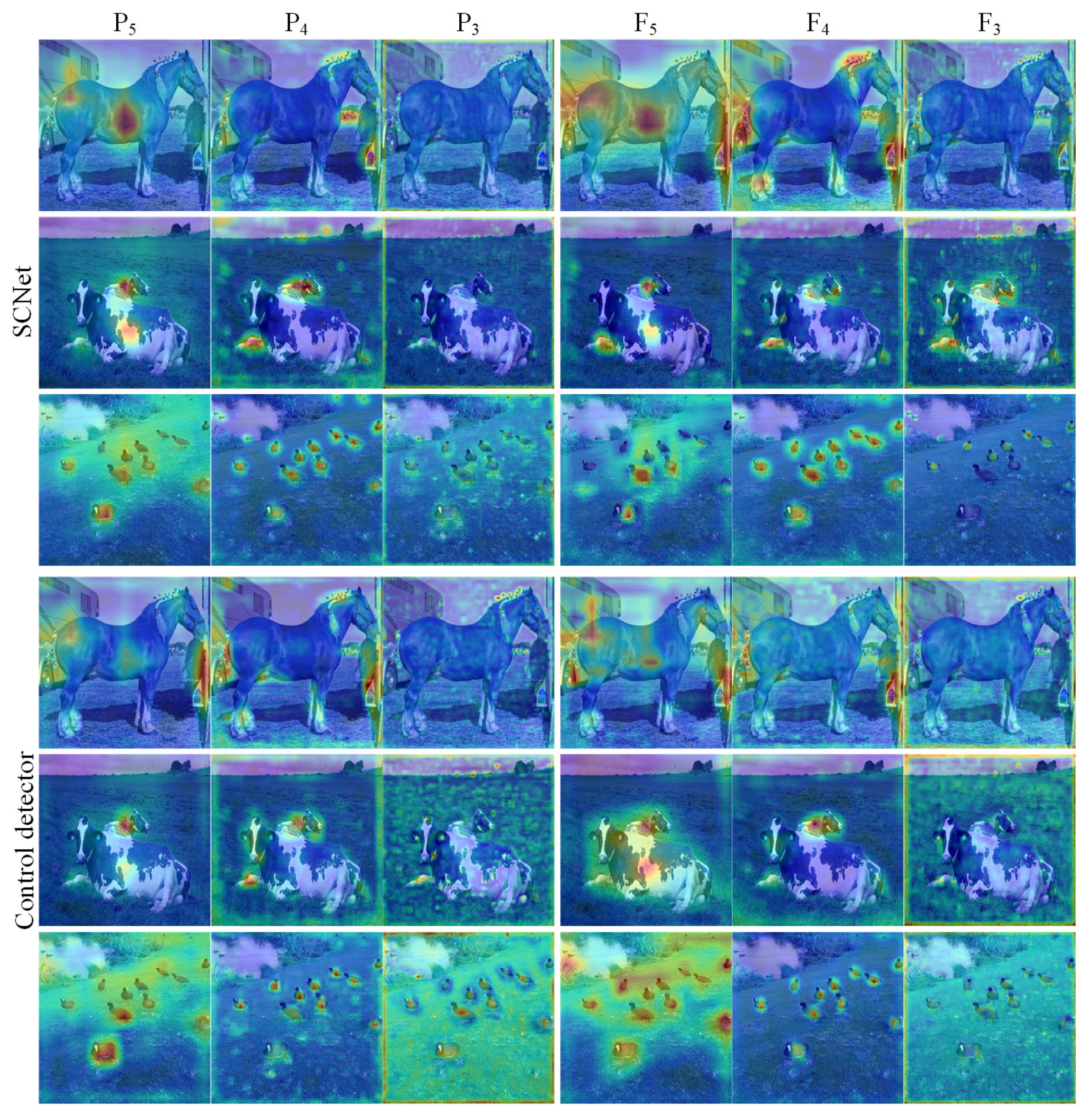
In order to further explore the facilitating role of our SC block in feature fusion, we compare the heat maps of multiple feature maps at different depth. Figure 8 demonstrates the qualitative results of feature maps . Map the values calculated by channel-wise summation to input images to obtain the heat maps of feature maps. The color scheme we adopted is the warm-to-cool color scheme, where the warm colors represent areas of more interest to the network and the cool colors represent areas of less interest to the network. On a whole, the overriding concern of the network is the central area of the object. As shown in the first row of Figure 8, the horse attracts great attention from the feature maps due to the large size. On the contrary, feature maps and take no notice of the object and view them as the background. This indicates that the feature information in the corresponding area on the feature map and is filtered out and do not get involved in gradient propagation during training. However, it does not imply that these feature maps take no effect on the prediction of the horse; they facilitate precise localization. After SC-FPN, the network is more attentive to the central area of the horse as shown in , which is conducive to improve detection performance. The analogous circumstance can be observed in the heat maps of the second row. The feature maps and are responsible for detecting the two cows due to the different sizes. After feature fusion by SC-FPN, the feature maps and pay more attention to central areas which contain stronger semantic information; on the contrary, feature maps focus on the areas around the object which contain more geometric information.
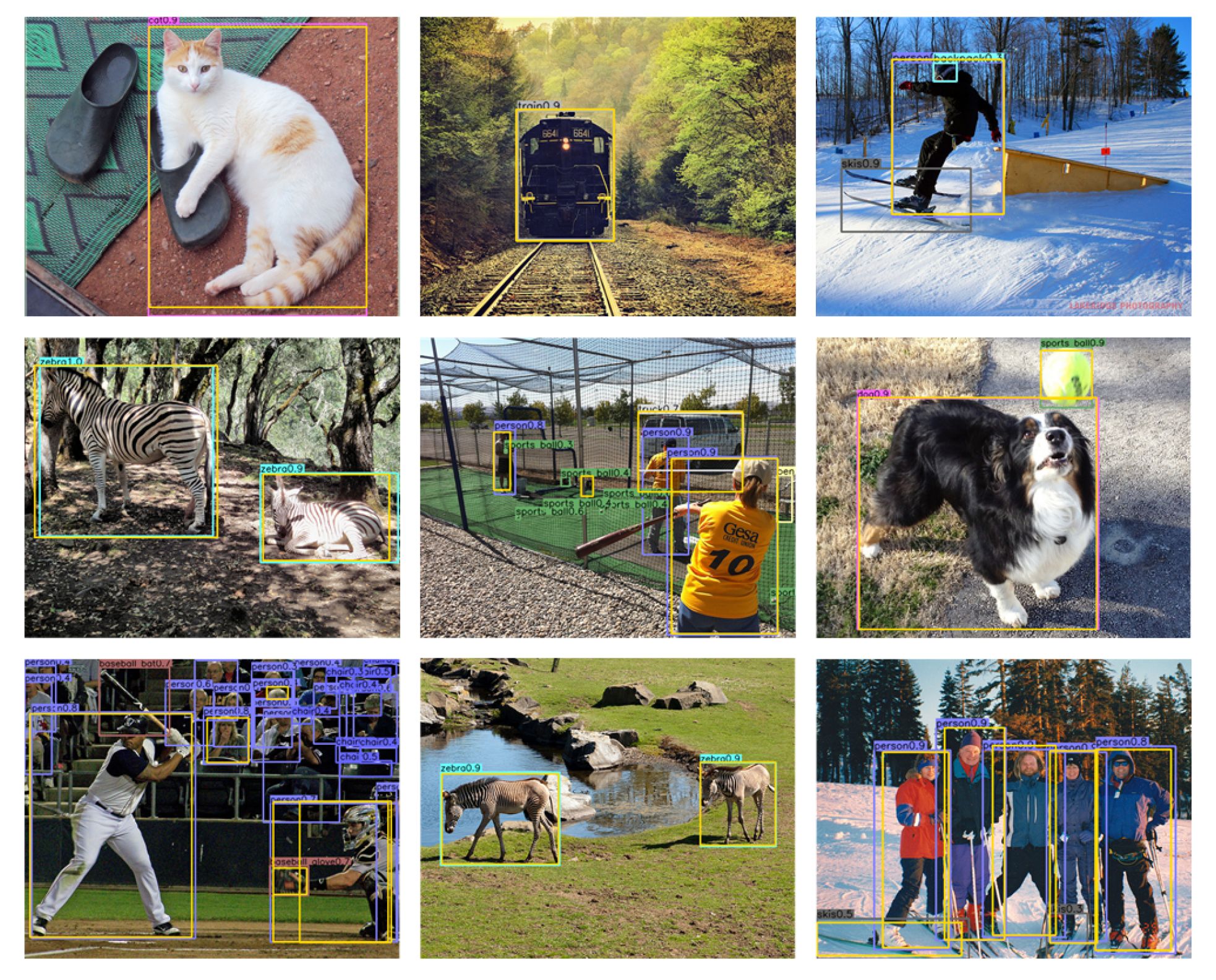
More experiments are added to verify that the good performance of SCNet is mainly due to SC modules, rather than these tricks. The same visualization is performed on a control detector which has exactly the same network structure and tricks as SCNet except for the SC block. The control detector adopts residual block to replace SC block in the backbone, and keeps almost the same number of trainable parameters and convolutional layers as SCNet to achieve a fair comparison. Take the third and sixth rows of Figure 8 as examples. Due to varying sizes, these objects are jointly predicted by three levels of feature maps. The full attention to the center areas reflects the good performance of SCNet, and, after SC-FPN processing, feature maps are more sensitive to critical areas. As for control detector, the heat maps indicate the inferior quality of feature maps, such as the omission of extremely small objects in the upper left corner of the image. After using the SC-FPN, the performance gap becomes more apparent. The SC block leads to a noticeable performance improvement in the box AP from 34.2% to 38.8% on the COCO val split, as shown in Table 3. Some examples of object detection results on the MS COCO test-dev set using an SCNet and control detectors are shown in Figure 9.
4.3. Comparison to Other Detectors
The SCNet is compared with other excellent detectors on the COCO test-dev split, and detailed results can be found in Table 4. Like other detectors, SCNet can adjust input resolution to obtain different speed-accuracy trade-off. At 608 × 608 input resolution, SCNet achieves AP of 38.9% on COCO test-dev split and outperforms most other mentioned detectors. Our detector lags behind ATSS in terms of accuracy but is faster and demands less input information. Compared with CenterNet, our detector is also superior in speed. SCNet is 0.9% lower than Mask R-CNN in terms of AP; our method runs 3.6× faster. Figure 10 shows the comparison of the proposed SCNet and several one-stage object detectors on the COCO test-dev split. The SCNet achieves a good speed-accuracy trade-off, the performance is also very close to some excellent detectors while maintaining a high inference speed.
5. Conclusions
In this paper, a novel feature fusion block is designed to improve the quality of feature representation, referred to as an SC block. It evenly splits the input into several parts, and processes each part with different sampling branches, and then concatenates the output of each branch one by one hierarchically. This structure instructs the network to rank information based on its importance to the task, and can consequently improve the model efficiency. A backbone network and an FPN employing this unit are built to construct our one-stage detector SCNet. Enhanced with the latest training tricks and modules, SCNet exhibits good performance in both speed and accuracy on the COCO test-dev split, achieving an AP of 38.9% with 40 FPS. Experimental results illustrate that the proposed block can generate strong discriminative features and improve the detection performance of the network. The SC block is scalable, simple, and effective. In addition, this unit may potentially provide a new idea of network construction for object detection and other visual tasks.
Author Contributions
Conceptualization, H.W. and D.L.; methodology, H.W. and D.L.; software, Y.S. and Q.G.; validation, H.W., D.L., and Y.S.; formal analysis, H.W. and Y.S.; investigation, H.W.; resources, D.L.; data curation, Y.S. and Q.G.; writing—original draft preparation, H.W. and Y.S.; writing—review and editing, Y.S. and Z.W.; visualization, Z.W.; supervision, Z.W. and C.L.; project administration, Z.W. and C.L.; funding acquisition, Q.G. and C.L. All authors have read and agreed to the published version of the manuscript.
Funding
This work was supported by the Fundamental Research on Advanced Technology and Engineering Application Team, Tianjin, China, under Grant No. 20160524.
Conflicts of Interest
The authors declare no conflict of interest.
References
- Liu, L.; Ouyang, W.; Wang, X.; Fieguth, P.; Chen, J.; Liu, X.; Pietikäinen, M. Deep learning for generic object detection: A survey. Int. J. Comput. Vis. 2020, 128, 261–318. [Google Scholar] [CrossRef] [Green Version]
- Wang, C.Y.; Mark Liao, H.Y.; Wu, Y.H.; Chen, P.Y.; Hsieh, J.W.; Yeh, I.H. CSPNet: A new backbone that can enhance learning capability of cnn. In Proceedings of the IEEE/CVF Conference on Computer Vision and Pattern Recognition Workshops, Seattle, WA, USA, 14–19 June 2020; pp. 390–391. [Google Scholar]
- Tan, M.; Le, Q.V. Efficientnet: Rethinking model scaling for convolutional neural networks. arXiv 2019, arXiv:1905.11946. [Google Scholar]
- He, K.; Zhang, X.; Ren, S.; Sun, J. Deep residual learning for image recognition. In Proceedings of the IEEE Conference on Computer Vision and Pattern Recognition, Las Vegas, NV, USA, 27–30 June 2016; pp. 770–778. [Google Scholar]
- Huang, G.; Liu, Z.; Pleiss, G.; Van Der Maaten, L.; Weinberger, K. Convolutional networks with dense connectivity. IEEE Trans. Pattern Anal. Mach. Intell. 2019. [Google Scholar] [CrossRef] [PubMed] [Green Version]
- Yu, F.; Wang, D.; Shelhamer, E.; Darrell, T. Deep layer aggregation. In Proceedings of the IEEE Conference on Computer Vision and Pattern Recognition, Salt Lake City, UT, USA, 18–22 June 2018; pp. 2403–2412. [Google Scholar]
- Newell, A.; Yang, K.; Deng, J. Stacked hourglass networks for human pose estimation. In European Conference on Computer Vision; Springer: Amsterdam, The Netherlands, 2016; pp. 483–499. [Google Scholar]
- Lin, T.Y.; Dollár, P.; Girshick, R.; He, K.; Hariharan, B.; Belongie, S. Feature pyramid networks for object detection. In Proceedings of the IEEE Conference on Computer Vision and Pattern Recognition, Honolulu, HI, USA, 21–26 July 2017; pp. 2117–2125. [Google Scholar]
- Liu, S.; Huang, D.; Wang, Y. Learning spatial fusion for single-shot object detection. arXiv 2019, arXiv:1911.09516. [Google Scholar]
- Zhao, Q.; Sheng, T.; Wang, Y.; Tang, Z.; Chen, Y.; Cai, L.; Ling, H. M2det: A single-shot object detector based on multi-level feature pyramid network. In Proceedings of the AAAI Conference on Artificial Intelligence, Honolulu, HI, USA, 27 January–1 February 2019; Volume 33, pp. 9259–9266. [Google Scholar]
- Hu, J.; Shen, L.; Sun, G. Squeeze-and-excitation networks. In Proceedings of the IEEE Conference on Computer Vision and Pattern Recognition, Salt Lake City, UT, USA, 18–22 June 2018; pp. 7132–7141. [Google Scholar]
- Dai, J.; Qi, H.; Xiong, Y.; Li, Y.; Zhang, G.; Hu, H.; Wei, Y. Deformable convolutional networks. In Proceedings of the IEEE International Conference on Computer Vision, Venice, Italy, 22–29 October 2017; pp. 764–773. [Google Scholar]
- Zhu, X.; Hu, H.; Lin, S.; Dai, J. Deformable convnets v2: More deformable, better results. In Proceedings of the IEEE Conference on Computer Vision and Pattern Recognition, Long Beach, CA, USA, 16–20 June 2019; pp. 9308–9316. [Google Scholar]
- Lin, T.Y.; Maire, M.; Belongie, S.; Hays, J.; Perona, P.; Ramanan, D.; Dollár, P.; Zitnick, C.L. Microsoft coco: Common objects in context. In European Conference on Computer Vision; Springer: Zurich, Switzerland, 2014; pp. 740–755. [Google Scholar]
- Girshick, R.; Donahue, J.; Darrell, T.; Malik, J. Rich feature hierarchies for accurate object detection and semantic segmentation. In Proceedings of the IEEE Conference on Computer Vision and Pattern Recognition, Columbus, OH, USA, 24–27 June 2014; pp. 580–587. [Google Scholar]
- Girshick, R. Fast r-cnn. In Proceedings of the IEEE International Conference on Computer Vision, Santiago, Chile, 7–13 December 2015; pp. 1440–1448. [Google Scholar]
- Ren, S.; He, K.; Girshick, R.; Sun, J. Faster r-cnn: Towards real-time object detection with region proposal networks. In Proceedings of the Advances in Neural Information Processing Systems, Montreal, QC, Canada, 7–12 December 2015; pp. 91–99. [Google Scholar]
- He, K.; Gkioxari, G.; Dollár, P.; Girshick, R. Mask r-cnn. In Proceedings of the IEEE International Conference on Computer Vision, Venice, Italy, 22–29 October 2017; pp. 2961–2969. [Google Scholar]
- Dai, J.; Li, Y.; He, K.; Sun, J. R-fcn: Object detection via region-based fully convolutional networks. In Proceedings of the Advances in Neural Information Processing Systems, Barcelona, Spain, 5–10 December 2016; pp. 379–387. [Google Scholar]
- Cai, Z.; Vasconcelos, N. Cascade r-cnn: Delving into high quality object detection. In Proceedings of the IEEE Conference on Computer Vision and Pattern Recognition, Salt Lake City, UT, USA, 18–22 June 2018; pp. 6154–6162. [Google Scholar]
- Sermanet, P.; Eigen, D.; Zhang, X.; Mathieu, M.; Fergus, R.; LeCun, Y. Overfeat: Integrated recognition, localization and detection using convolutional networks. arXiv 2013, arXiv:1312.6229. [Google Scholar]
- Redmon, J.; Divvala, S.; Girshick, R.; Farhadi, A. You only look once: Unified, real-time object detection. In Proceedings of the IEEE Conference on Computer Vision and Pattern Recognition, Las Vegas, NV, USA, 27–30 June 2016; pp. 779–788. [Google Scholar]
- Redmon, J.; Farhadi, A. YOLO9000: Better, faster, stronger. In Proceedings of the IEEE Conference on Computer Vision and Pattern Recognition, Honolulu, HI, USA, 21–26 July 2017; pp. 7263–7271. [Google Scholar]
- Redmon, J.; Farhadi, A. Yolov3: An incremental improvement. arXiv 2018, arXiv:1804.02767. [Google Scholar]
- Liu, W.; Anguelov, D.; Erhan, D.; Szegedy, C.; Reed, S.; Fu, C.Y.; Berg, A.C. Ssd: Single shot multibox detector. In European Conference on Computer Vision; Springer: Amsterdam, The Netherlands, 2016; pp. 21–37. [Google Scholar]
- Lin, T.Y.; Goyal, P.; Girshick, R.; He, K.; Dollár, P. Focal loss for dense object detection. In Proceedings of the IEEE International Conference on Computer Vision, Venice, Italy, 22–29 October 2017; pp. 2980–2988. [Google Scholar]
- Li, B.; Liu, Y.; Wang, X. Gradient harmonized single-stage detector. In Proceedings of the AAAI Conference on Artificial Intelligence, Honolulu, HI, USA, 27 January–1 February 2019; Volume 33, pp. 8577–8584. [Google Scholar]
- Tian, Z.; Shen, C.; Chen, H.; He, T. Fcos: Fully convolutional one-stage object detection. In Proceedings of the IEEE International Conference on Computer Vision, Seoul, Korea, 27 October–2 November 2019; pp. 9627–9636. [Google Scholar]
- Law, H.; Deng, J. Cornernet: Detecting objects as paired keypoints. In Proceedings of the European Conference on Computer Vision (ECCV), Munich, Germany, 8–14 September 2018; pp. 734–750. [Google Scholar]
- Zhou, X.; Zhuo, J.; Krahenbuhl, P. Bottom-up object detection by grouping extreme and center points. In Proceedings of the IEEE Conference on Computer Vision and Pattern Recognition, Long Beach, CA, USA, 16–20 June 2019; pp. 850–859. [Google Scholar]
- Duan, K.; Bai, S.; Xie, L.; Qi, H.; Huang, Q.; Tian, Q. Centernet: Keypoint triplets for object detection. In Proceedings of the IEEE International Conference on Computer Vision, Seoul, Korea, 27 October–2 November 2019; pp. 6569–6578. [Google Scholar]
- Zhou, X.; Wang, D.; Krähenbühl, P. Objects as points. arXiv 2019, arXiv:1904.07850. [Google Scholar]
- Bochkovskiy, A.; Wang, C.Y.; Liao, H.Y.M. YOLOv4: Optimal Speed and Accuracy of Object Detection. arXiv 2020, arXiv:2004.10934. [Google Scholar]
- Liu, S.; Qi, L.; Qin, H.; Shi, J.; Jia, J. Path aggregation network for instance segmentation. In Proceedings of the IEEE Conference on Computer Vision and Pattern Recognition, Salt Lake City, UT, USA, 18–22 June 2018; pp. 8759–8768. [Google Scholar]
- Tan, M.; Pang, R.; Le, Q.V. Efficientdet: Scalable and efficient object detection. In Proceedings of the IEEE/CVF Conference on Computer Vision and Pattern Recognition, Seattle, WA, USA, 13–19 June 2020; pp. 10781–10790. [Google Scholar]
- Wang, J.; Chen, K.; Yang, S.; Loy, C.C.; Lin, D. Region proposal by guided anchoring. In Proceedings of the IEEE Conference on Computer Vision and Pattern Recognition, Long Beach, CA, USA, 5–20 June 2019; pp. 2965–2974. [Google Scholar]
- Zhang, S.; Chi, C.; Yao, Y.; Lei, Z.; Li, S.Z. Bridging the gap between anchor-based and anchor-free detection via adaptive training sample selection. In Proceedings of the IEEE/CVF Conference on Computer Vision and Pattern Recognition, Seattle, WA, USA, 13–19 June 2020; pp. 9759–9768. [Google Scholar]
- Rezatofighi, H.; Tsoi, N.; Gwak, J.; Sadeghian, A.; Reid, I.; Savarese, S. Generalized intersection over union: A metric and a loss for bounding box regression. In Proceedings of the IEEE Conference on Computer Vision and Pattern Recognition, Long Beach, CA, USA, 16–20 June 2019; pp. 658–666. [Google Scholar]
- Kingma, D.P.; Ba, J. Adam: A method for stochastic optimization. arXiv 2014, arXiv:1412.6980. [Google Scholar]
- Zhang, Z.; He, T.; Zhang, H.; Zhang, Z.; Xie, J.; Li, M. Bag of freebies for training object detection neural networks. arXiv 2019, arXiv:1902.04103. [Google Scholar]
- He, T.; Zhang, Z.; Zhang, H.; Zhang, Z.; Xie, J.; Li, M. Bag of tricks for image classification with convolutional neural networks. In Proceedings of the IEEE Conference on Computer Vision and Pattern Recognition, Long Beach, CA, USA, 16–20 June 2019; pp. 558–567. [Google Scholar]
- He, K.; Zhang, X.; Ren, S.; Sun, J. Delving deep into rectifiers: Surpassing human-level performance on imagenet classification. In Proceedings of the IEEE International Conference on Computer vision, Santiago, Chile, 7–13 December 2015; pp. 1026–1034. [Google Scholar]
- Deng, J.; Dong, W.; Socher, R.; Li, L.J.; Li, K.; Fei-Fei, L. Imagenet: A large-scale hierarchical image database. In Proceedings of the 2009 IEEE Conference on Computer Vision and Pattern Recognition, Miami, FL, USA, 20–25 June 2009; pp. 248–255. [Google Scholar]
- Yao, Z.; Cao, Y.; Zheng, S.; Huang, G.; Lin, S. Cross-iteration batch normalization. arXiv 2020, arXiv:2002.05712. [Google Scholar]
- Misra, D. Mish: A self regularized non-monotonic neural activation function. arXiv 2019, arXiv:1908.08681. [Google Scholar]
- Yun, S.; Han, D.; Oh, S.J.; Chun, S.; Choe, J.; Yoo, Y. Cutmix: Regularization strategy to train strong classifiers with localizable features. In Proceedings of the IEEE International Conference on Computer Vision, Seoul, Korea, 27 October–2 November 2019; pp. 6023–6032. [Google Scholar]
- Ghiasi, G.; Lin, T.Y.; Le, Q.V. Dropblock: A regularization method for convolutional networks. In Proceedings of the Advances in Neural Information Processing Systems, Montréal, QC, Canada, 3–8 December 2018; pp. 10727–10737. [Google Scholar]
- He, K.; Zhang, X.; Ren, S.; Sun, J. Spatial pyramid pooling in deep convolutional networks for visual recognition. IEEE Trans. Pattern Anal. Mach. Intell. 2015, 37, 1904–1916. [Google Scholar] [CrossRef] [Green Version]
- Bodla, N.; Singh, B.; Chellappa, R.; Davis, L.S. Soft-NMS–improving object detection with one line of code. In Proceedings of the IEEE International Conference on Computer Vision, Venice, Italy, 22–29 October 2017; pp. 5561–5569. [Google Scholar]
- Ioffe, S.; Szegedy, C. Batch normalization: Accelerating deep network training by reducing internal covariate shift. arXiv 2015, arXiv:1502.03167. [Google Scholar]
Figure 1.
A Split-and-Combine block.

Figure 2.
SC blocks with different configurations. (a) SC-(2,1,2); (b) SC-(3,2,2,4); (c) SC-(4,2,2,4,6); (d) SC-(4,2,2,4,8).
Figure 2.
SC blocks with different configurations. (a) SC-(2,1,2); (b) SC-(3,2,2,4); (c) SC-(4,2,2,4,6); (d) SC-(4,2,2,4,8).

Figure 3.
The structure of the SC-59 network which consists of five SC blocks and five residual blocks. We employ residual blocks to complete downsampling operations. The output of the last three SC blocks is extracted to construct a feature pyramid network.
Figure 3.
The structure of the SC-59 network which consists of five SC blocks and five residual blocks. We employ residual blocks to complete downsampling operations. The output of the last three SC blocks is extracted to construct a feature pyramid network.

Figure 4.
The structure of our detector. It employs an SC block to build a backbone network and SC-FPN. The fused feature maps are then delivered to a sub-network to generate dense predictions of boundary box locations and categories.
Figure 4.
The structure of our detector. It employs an SC block to build a backbone network and SC-FPN. The fused feature maps are then delivered to a sub-network to generate dense predictions of boundary box locations and categories.

Figure 5.
Illustration of network design. (a) PANet; (b) our SC-PANet; (c) our SC-fusion block.

Figure 6.
Positive samples selection for training. Ground truth boxes (in red) still have high IoU with prediction boxes (in blue), although their centers are positive (in red mask) and negative (in blue mask), respectively.
Figure 6.
Positive samples selection for training. Ground truth boxes (in red) still have high IoU with prediction boxes (in blue), although their centers are positive (in red mask) and negative (in blue mask), respectively.

Figure 7.
The examples of Admix, we mix information from five images at once to implement data augmentation.
Figure 7.
The examples of Admix, we mix information from five images at once to implement data augmentation.

Figure 8.
Heat maps of feature maps , which are extracted from SCNet and a control detector. These detectors complete the network training under the same conditions and tricks to achieve fair comparisons.
Figure 8.
Heat maps of feature maps , which are extracted from SCNet and a control detector. These detectors complete the network training under the same conditions and tricks to achieve fair comparisons.

Figure 9.
Some detection results of SCNet on the MS COCO test-dev set. The gold boxes indicate the detection results of the control detector.
Figure 9.
Some detection results of SCNet on the MS COCO test-dev set. The gold boxes indicate the detection results of the control detector.

Figure 10.
FPS vs. Average Precision on COCO test-dev. SCNet lags behind ATSS and CenterNet in terms of accuracy but is superior in speed. The proposed SCNet exhibits good speed-accuracy trade-off compared with other algorithms.
Figure 10.
FPS vs. Average Precision on COCO test-dev. SCNet lags behind ATSS and CenterNet in terms of accuracy but is superior in speed. The proposed SCNet exhibits good speed-accuracy trade-off compared with other algorithms.


Table 1.
The effect of each trick on the baseline network. All of the listed design decisions generate presentable performance gains in AP—evaluated on the COCO val split.
Table 1.
The effect of each trick on the baseline network. All of the listed design decisions generate presentable performance gains in AP—evaluated on the COCO val split.
| Baseline | SCNet | |||||||
|---|---|---|---|---|---|---|---|---|
| CmBN | √ | √ | √ | √ | √ | √ | √ | |
| Mish | √ | √ | √ | √ | √ | √ | ||
| Admix | √ | √ | √ | √ | √ | |||
| warmup+cosine | √ | √ | √ | √ | ||||
| multi-scale training | √ | √ | √ | |||||
| GA | √ | √ | ||||||
| DropBlock+SPP | √ | |||||||
| COCO val AP | 32.1 | 33.3 | 34.1 | 35.2 | 35.9 | 36.8 | 37.7 | 38.8 |
| FPS | 46 | 46 | 46 | 46 | 46 | 46 | 44 | 40 |
Table 2.
Speed-accuracy trade off with different backbone networks, the results are tested on the COCO val split.
Table 2.
Speed-accuracy trade off with different backbone networks, the results are tested on the COCO val split.
| Backbone | FPS | Input Size | AP | ||||||
|---|---|---|---|---|---|---|---|---|---|
| SCNet | SC-32 | 67.0 | 416 × 416 | 27.6 | 46.3 | 29.4 | 8.7 | 31.5 | 41.0 |
| SCNet | SC-32 | 65.8 | 608 × 608 | 29.3 | 48.0 | 33.3 | 10.3 | 32.5 | 42.8 |
| SCNet | SC-47 | 60.5 | 416 × 416 | 32.6 | 50.5 | 34.9 | 15.4 | 36.9 | 46.4 |
| SCNet | SC-47 | 54.7 | 608 × 608 | 34.7 | 52.8 | 37.4 | 16.9 | 39.3 | 48.4 |
| SCNet | SC-59 | 51.0 | 416 × 416 | 37.1 | 55.0 | 40.3 | 18.5 | 40.9 | 48.9 |
| SCNet | SC-59 | 40.0 | 608 × 608 | 38.8 | 56.7 | 42.5 | 19.6 | 42.7 | 51.0 |
Table 3.
Comparison of SCNet and control detector—evaluated on a COCO val split.
| AP | ||||||
|---|---|---|---|---|---|---|
| control detector | 34.2 | 53.0 | 37.4 | 18.0 | 38.8 | 46.4 |
| SCNet | 38.8 | 56.7 | 42.5 | 19.6 | 42.7 | 51.0 |
Table 4.
Detection performance tested on COCO test-dev. The following table summarizes some two-stage detectors and one-stage detectors. The FPS of all mentioned detectors are measured on RTX 2080ti GPU, and the performance measure data are copied from the original publication. Our SCNet is in bold.
| Backbone | FPS | Input Size | AP | ||||||
|---|---|---|---|---|---|---|---|---|---|
| Two-stage detectors | |||||||||
| Faster R-CNN +++ | ResNet-101 | – | 1000 × 600 | 34.9 | 55.7 | 37.4 | 15.6 | 38.7 | 50.9 |
| Faster R-CNN w FPN | ResNet-101-FPN | – | 1000 × 600 | 36.2 | 59.1 | 39.0 | 18.2 | 39.0 | 48.2 |
| Mask R-CNN | ResNeXt-101 | 9.0 | 1333 × 800 | 39.8 | 62.3 | 43.4 | 22.1 | 43.2 | 51.2 |
| One-stage detectors | |||||||||
| SSD | VGG | 40.9 | 300 × 300 | 25.1 | 43.1 | 25.8 | – | – | – |
| SSD | VGG | 20.9 | 512 × 512 | 28.8 | 48.5 | 30.3 | – | – | – |
| YOLOv2 | DarkNet-19 | 40.0 | 544 × 544 | 21.6 | 44.0 | 19.2 | 5.0 | 22.4 | 35.5 |
| YOLOv3 | darknet-53 | 19.0 | 608 × 608 | 33.0 | 57.9 | 34.4 | 18.3 | 35.4 | 41.9 |
| RefineDet | VGG | 36.8 | 320 × 320 | 29.4 | 49.2 | 31.3 | 10.0 | 32.0 | 44.4 |
| RefineDet | VGG | 21.2 | 512 × 512 | 33.0 | 54.5 | 35.5 | 16.3 | 36.3 | 44.3 |
| CenterNet-DLA | DLA-34 | 26.9 | 512 × 512 | 39.2 | 57.1 | 42.8 | 19.9 | 43.0 | 51.4 |
| CenterNet-HG | Hourglass-104 | 7.4 | 512 × 512 | 42.1 | 61.1 | 45.9 | 24.1 | 45.5 | 52.8 |
| RetinaNet | ResNet-101-FPN | 5.0 | 800 × 800 | 39.1 | 59.1 | 42.3 | 21.8 | 42.7 | 50.2 |
| ATSS | ResNet-101 | 14.9 | 800 × 800 | 43.6 | 62.1 | 47.4 | 26.1 | 47.0 | 53.6 |
| ATSS | ResNet-101-DCN | 11.7 | 800 × 800 | 46.3 | 64.7 | 50.4 | 27.7 | 49.8 | 58.4 |
| SCNet(ours) | SC-59 | 51.0 | 416 × 416 | 37.1 | 54.9 | 40.4 | 18.5 | 40.9 | 48.9 |
| SCNet(ours) | SC-59 | 40.0 | 608 × 608 | 38.9 | 56.8 | 42.6 | 19.7 | 42.7 | 51.1 |
© 2020 by the authors. Licensee MDPI, Basel, Switzerland. This article is an open access article distributed under the terms and conditions of the Creative Commons Attribution (CC BY) license (http://creativecommons.org/licenses/by/4.0/).
Share and Cite
MDPI and ACS Style
Wang, H.; Li, D.; Song, Y.; Gao, Q.; Wang, Z.; Liu, C. Single-Shot Object Detection with Split and Combine Blocks. Appl. Sci. 2020, 10, 6382. https://0-doi-org.brum.beds.ac.uk/10.3390/app10186382
AMA Style
Wang H, Li D, Song Y, Gao Q, Wang Z, Liu C. Single-Shot Object Detection with Split and Combine Blocks. Applied Sciences. 2020; 10(18):6382. https://0-doi-org.brum.beds.ac.uk/10.3390/app10186382
Chicago/Turabian StyleWang, Hongwei, Dahua Li, Yu Song, Qiang Gao, Zhaoyang Wang, and Chunping Liu. 2020. "Single-Shot Object Detection with Split and Combine Blocks" Applied Sciences 10, no. 18: 6382. https://0-doi-org.brum.beds.ac.uk/10.3390/app10186382
Note that from the first issue of 2016, this journal uses article numbers instead of page numbers. See further details here.