NAP: Natural App Processing for Predictive User Contexts in Mobile Smartphones


1
Department of Software, Sungkyunkwan University, Suwon 16419, Korea
2
Department of Computer Science, Chungbuk National University, Cheongju 28644, Korea
*
Authors to whom correspondence should be addressed.
Appl. Sci. 2020, 10(19), 6657; https://0-doi-org.brum.beds.ac.uk/10.3390/app10196657
Submission received: 15 July 2020
/
Revised: 16 September 2020
/
Accepted: 19 September 2020
/
Published: 23 September 2020
(This article belongs to the Collection Big Data Analysis and Visualization Ⅱ)
Abstract
:The resource management of an application is an essential task in smartphones. Optimizing the application launch process results in a faster and more efficient system, directly impacting the user experience. Predicting the next application that will be used can orient the smartphone to address the system resources to the correct application, making the system more intelligent and efficient. Neural networks have been presenting outstanding results in the state-of-the-art for mapping large sequences of data, outperforming all previous classification and prediction models. A recurrent neural network (RNN) is an artificial neural network associated with sequence models, and it can recognize patterns in sequences. One of the areas that use RNN is language modeling (LM). Given an arrangement of words, LM can learn how the words are organized in sentences, making it possible to predict the next word given a group of previous words. We propose building a predictive model inspired by LM. However, instead of using words, we will use previous applications to predict the next application. Moreover, some context features, such as timestamp and energy record, will be included in the prediction model to evaluate the impact of the features on the performance. We will provide the following application prediction result and extend it to the top-k possible candidates for the next application.
1. Introduction
The recent and brief history of smartphones is mainly marked by rapid technological growth. Both hardware and software have significantly improved in recent years, enabling and motivating the development of new applications (apps). It is estimated that the Google Play Store had more than 2.5 million apps available in 2019 [1]. Together with the massive number of apps available, the number of apps installed is also increasing significantly. It is estimated that smartphone users install more than 150 apps on their devices [2].
Given this scenario with many apps installed, optimizing the app management is essential if we want to deliver an efficient system to the user. Searching for an app becomes not practical, making the user spend a lot of time until finding the app. This motivated researchers to develop app prediction methods, such as FALCON [3], which are based on context signals and user access patterns. Another important issue is resource allocation in smartphones. If we can predict the app usage behavior, it is possible to assign the required resources in advance to the expected app. For instance, it is possible to preload the app in memory or avoid the system to kill the next app to be used in situations when memory is saturated [4].
To build an efficient app prediction model, it is essential to analyze the user’s behavior over time. For instance, does the user typically change the most used apps along time? How relevant are the most used apps in the prediction task? If it is possible to use context features, such as time and smartphone energy status, it will help in the app prediction? In this work, we propose to discuss these questions using a neural network applied to a long app usage dataset record. The idea is to treat the app usage dataset as sequential data, where we want to predict the next application given a sequence of previous applications used.
Neural networks can collect knowledge from the data set and establish a relationship between the input and the prediction. One kind of neural network often used to process sequence data is the Recurrent Neural Network (RNN). One of the RNN’s features is to predict the next element of a sequence. For instance, predict a company’s share price given its history on the stock market, or perform a weather forecast given the previous weather conditions [5]. These examples are in the time-series prediction group, which means the dataset is following a timeline sequence. Another example, where RNN is often used is in language modeling (LM). LM represents probabilistic models that can predict the next word in the sequence given the words that precede it [6]. Since words follow communication patterns to build sentences, we can use RNN to learn these patterns and use them to predict the next word. For instance, if we try to predict the next word in the sentence “Please, give me a glass of…”, the most probable word might be “water” due to the sentence pattern used in the English language. If we extend to multiple possible candidates, we can say that “water, juice and soda” might be good candidates for the given sentence.
In this work, we build a model to predict the next application based on the LM approach, the Natural App Processing (NAP). If it is possible to correlate the applications and features as words in sentences, we can reproduce the word prediction task to the app prediction problem. First, we process the apps and features as words using the tokenization and encoding. The encoded are used as input to the RNN. The RNN output is processed by a softmax function to give the prediction. In the end, we evaluate the prediction using categorical cross-entropy. We used a dataset with 34 users containing app usage ranging from 6 to 14 months. We evaluate the app usage monthly for all users, and we got 86.58% accuracy in the app prediction using Recall@5.
This paper has the following orientation. First, we briefly present the methods used in previous works and their interpretation of the application prediction problem. We also show details about the dataset and their results. After, we explain the app prediction model based on LM and how the app usage is distributed across the dataset used. We evaluate our model and compare it with other approaches, and then, we finalize with the conclusions.
2. Related Work
In recent years, several studies have been done regarding app prediction. Many of these studies were inspired by models that achieved a recognized success in different areas, such as character prediction and recommendation systems. Moreover, some attempts have been made to ascertain whether contextual information is related to applications’ use.
The first attempts were applying traditional machine learning techniques with contextual information to the app prediction problem. Yan et al. [3], introduced the FALCON model, based on the cost-benefit learning algorithm, where they used contexts as features to predict the application launches by the user, such as geographical position and temporal access patterns. They measured the average Recall for all users throw the days, and they achieved over 80% in Recall@5 after eight months of cumulative training data. However, Falcon does not address the fluctuation in test results along the time, and also, it is necessary long training time to achieve satisfactory results.
Nataranjan et al. [7] explored Markov models, assuming that an app’s choice is strongly related to the previous app used. They developed the IconRank algorithm based on the collaborative filtering model, which is used for recommendation systems. The idea was to model the app transition using a Markov chain for each user and then apply a clustering algorithm based on these transitions. The dataset used was one of the first works containing many users (total 17,062). The app usage is highly concentrated in a few applications, with 85% of the total launches concentrated in just 1% of the total apps. As a result, they achieved a Recall@5 of 67.01%. Build a model based on the previous state might not be the right choice if the user has a concentrated app distribution. We will show that the Least Recently Used (LRU) algorithm also performs poorly.
Parate et al. [8] also proposed another prediction model based on the Markov model. They built the App Prediction by Partial match (APPM) based on the prediction by partial match (PPM) used in character prediction [9]. PPM computes the conditional probability mapping of the characters in a sequence. The work highlighted the user behavior difference. For example, they found out that in some cases, a user tends to strongly favor recently used apps, whereas in other cases, a user exhibits highly sequential app usage behavior. The data set used was from the LiveLab project [10], where it has 34 users, and their app records with features such as time and position when using the app. They achieved 81.35% of Recall@5. While Markov models learn the correlation among the apps, they assumed the next app is only related to the latest app and ignored the multiple previous apps used.
Huang et al. [11] explored various contextual information, such as the last used app, time, location, and the user profile using a Bayesian framework. They argued that considering only the dependencies between the app usage behaviors is not enough, suggesting that the contexts should be included to better prediction accuracy. The Recall@5 was 69% using the MDC data set, which consists of 38 users and app usage records for more than one year. Bayesian models combine app usage with contextual features, and the features used are assumed to be independent. However, app usage is closely connected to contextual information.
With the advancement of neural networks in several areas, some researchers have begun to implement it in the app prediction task. Xu et al. [12] have proposed an LSTM model to explore the temporal-sequence dependency of the apps with contextual information. However, they did not explore some extensions of LSTM, such as the bidirectional LSTM. Moreover, they have only collected data within a month, which is a short period to evaluate the model’s performance.
Zhao et al. [13] proposed a scheme called AppUsage2Vec, which is inspired by Doc2Vec [14]. The idea is to represent app usage as a vector as it was done with words in Doc2Vec. Different from Doc2Vec, they included the time feature since some works have demonstrated a strong relationship between app usage and time. AppUsage2Vec consists of an app attention mechanism, which weights the most relevant apps and a dual deep neural network (DNN), which learns personalized app usage characteristics by each user. They tested their model using app records by 10,360 users for three months. The Recall@5 was 84.46%. Even though AppUsage2Vec achieved promising results using a dataset with many users, it was only tested for one month period. To reproduce a general model for the user, a long period analysis is more appropriated.
3. Natural App Processing Model
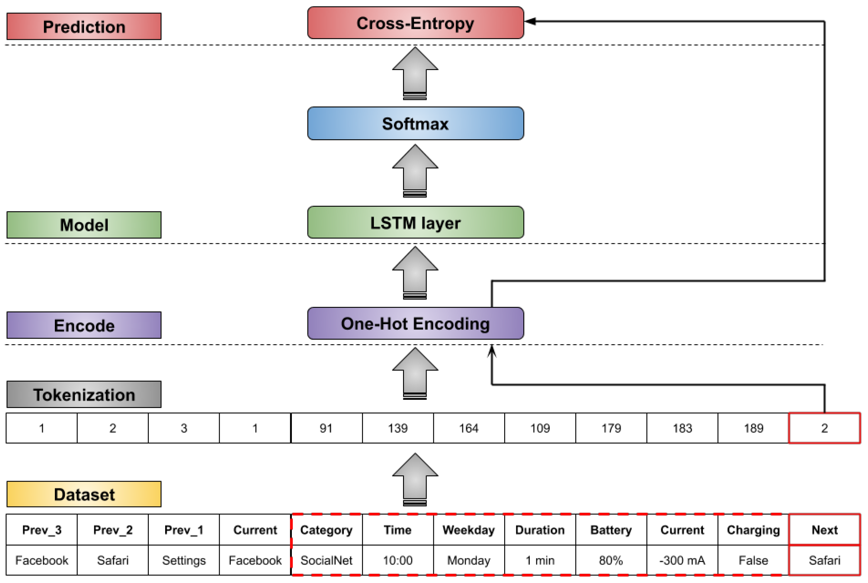
Our app prediction model is inspired by the LM using RNN. However, instead of using a sequence of words, we used the app usage records with their respective context features. The app category, time, duration, and battery information were the features used. As explored in [3,8], we aim to investigate the correlation between the apps and context features to improve the prediction results. For each app usage record, we include n number of previous apps used and the features regarding the current app record. The target is to predict the next app. Figure 1 shows an overview of our prediction model. The first part consists of arranging the app records with their respective previous apps, features, and future next app. After, it is necessary to convert these sequences elements into unique values. This process is called tokenization, which is covered in the following subsection.
3.1. Tokenization
As is done when processing words in LM, the apps and features will compose a dictionary with each app and feature represented by a unique token [15]. Since some features have a large range of values, the dictionary size can increase significantly. For instance, the battery level has values such as 92% and 93%. These two battery level data will be transformed into two unique tokens. Since 92% and 93% are very similar in terms of battery level, it is better to provide a unique token to represent both. To solve this problem, we established ranges such as 90% < x ≤ 100%, and now values inside this range are represented by a unique token. This procedure will reduce the dictionary size and the complexity of the context features. After the tokenization process, each token can be encoded.
3.2. Encoding
The one-hot encoding transforms categorical data into a vector representation. The vector is composed of zeros, with only one at the index of the data represented by the number. For example, a value 2 is transformed to a vector (0, 0,…, 1, 0) by the one-hot encoding. The total vector length is the dictionary size. The one-hot encoding is a fast and simple process. In our experiments, it performed better than the embedding method [16].
3.3. RNN and Prediction Output
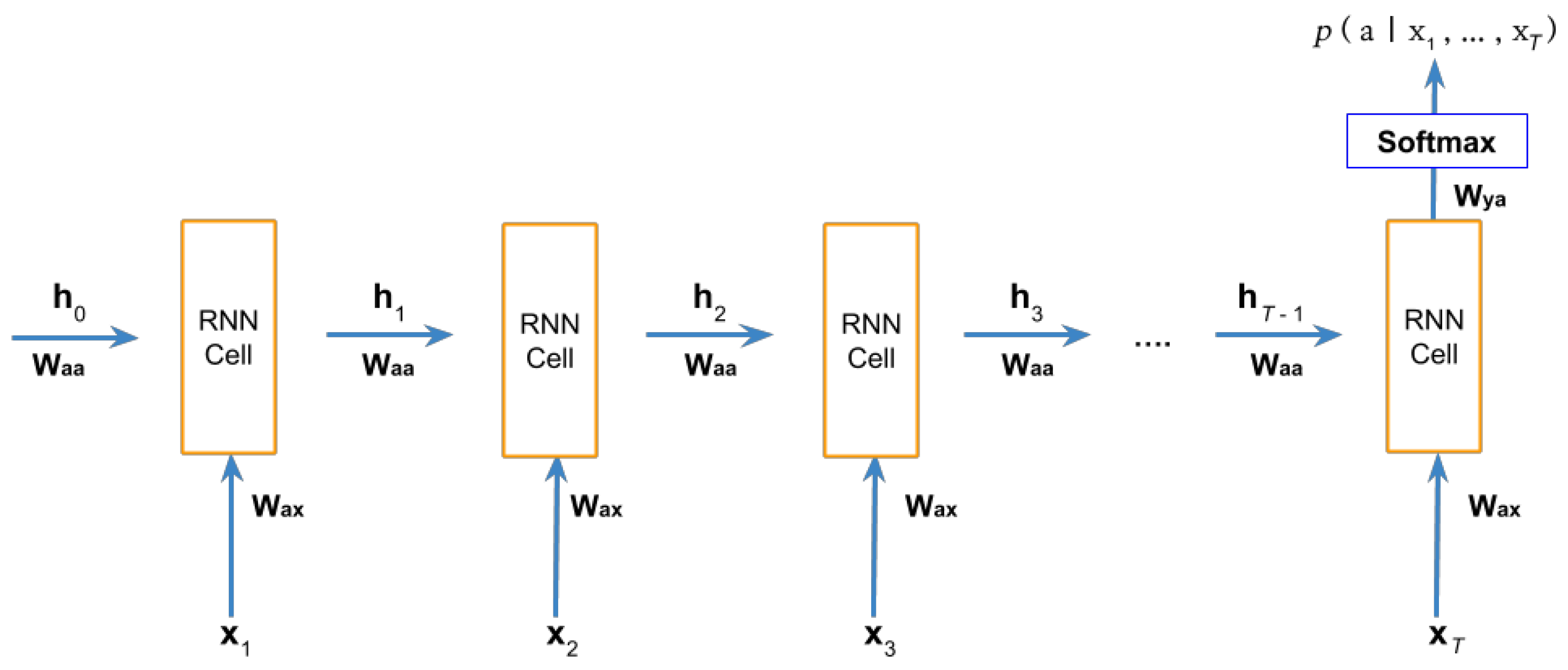
As explained in Section 2, RNN can learn patterns from a sequential dataset. Given a set of apps A and features F, we aim to implement a model that inputs a fixed-length sequence of apps and features and outputs the probability of an app a to be chosen, where . Formally, giving a sequence where , we can output the conditional probability , computing the feedforward propagation in RNN and using a softmax function, as represented in Figure 2 and also in the equations below:
where and are the weights and bias of the RNN respectively. g represents the activation function. For RNN, the common choice is the or , which helps to prevent the vanishing gradient problem [17]. Each RNN cell computes the input and the previous cell’s output , going throw all the apps and features. This configuration presenting in Figure 2 is known as many-to-one [18], where the input sequence is higher than one () and it outputs for only one cell. The softmax function normalizes the RNN output into a probability distribution consisting of K probabilities, where the K length is equal to the total number of elements in A. The equations below show the softmax computation:
where and are the weight and bias of the softmax function respectively. is the ith element of the z vector, where . The output from the softmax function will be a vector containing the probability for each app to be chosen, or in other words, the final prediction output :
However, this is the prediction for one input sequence. Giving M sequences, we want to compute the loss function for the multi-classification problem. In the case of word prediction, one widely used is the categorical cross-entropy. In order to optimize the weights and the bias , we should reduce the negative cross-entropy :
where is the training data. In 1997, the Long Short-Term Memory cell (LSTM) Hochreiter [19] was published, introducing the forgotten, update, and output gates. The LSTM has made a huge impact on sequence models and is adopted in many different tasks today(including language models). The gates improve the memorization task, including in long sequences examples. In this study, we will adopt the LSTM as the basic cell in our NAP model.
3.4. Data Set
The data set is provided by the LiveLab project from Rice University [10], which consists of 34 app usage traces. The app usage period ranges between 6 months until 14 months. The average number of apps used during the whole period by all users is 140, and the absolute number of apps used fluctuates from the minimum 40 to a maximum of 535 apps.
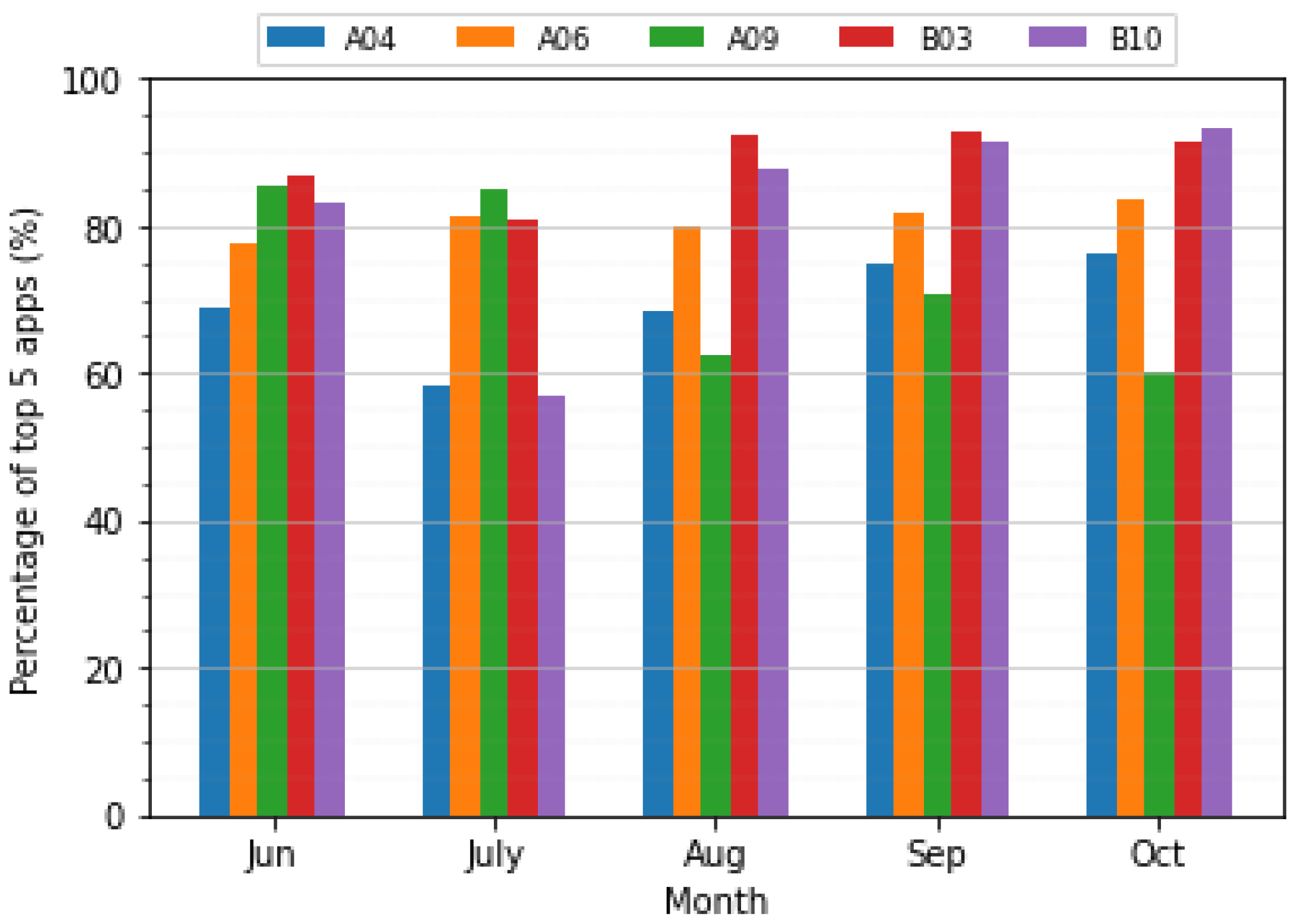
Since the data set is for an extended period, it interests to monitory the app usage behavior throw time steps. For instance, we can check periodically whether the users concentrate their app usage in a few apps or not. In Figure 3, it is shown the percentage of the top 5 apps used by 5 users from June until October. The top 5 apps percentage can change significantly during the months. Taking the A09 user from Figure 3, the top 5 apps represents 85% of all the records registered in June, while in October, this percentage drops to 60%. It indicates that the user changed from a few apps concentration to more balanced app usage. Even with this high variation, it is important to the prediction model account these 5 most-used apps. The reason is that the average percentage of the 5 most used apps for all the 34 users during the whole period is 74.75 %. Moreover, the top 5 apps are not constant over time. On average, 10 applications are among the five most-used applications over the user’s period.
3.5. Model Details
The NAP was developed using a deep learning API written in Python called Keras, running on top of the machine learning platform TensorFlow. The model is composed of 2 layers of LSTM, a dropout layer to reduce overfitting and a softmax layer to compute the prediction results. After tuning the number of hidden nodes, we find out that 64 and 32 for the first and second layer respectively, reduced the overfitting. We used the criterion of recall to measure the performance of our model. The recall was computed when top k apps with the highest probability were selected, namely Recall@k [13].
4. Evaluation
In the evaluation section, we first provide the monthly prediction for 5 users using our model. The reason is to highlight the different prediction tendencies from the users. After, we change the number of previous applications from 2 until 6 on the dataset to see if there is variation in the prediction results. We also evaluated whether the context features improve app prediction performance or not. Finally, we compare our results with three different models.
4.1. User Data Analysis
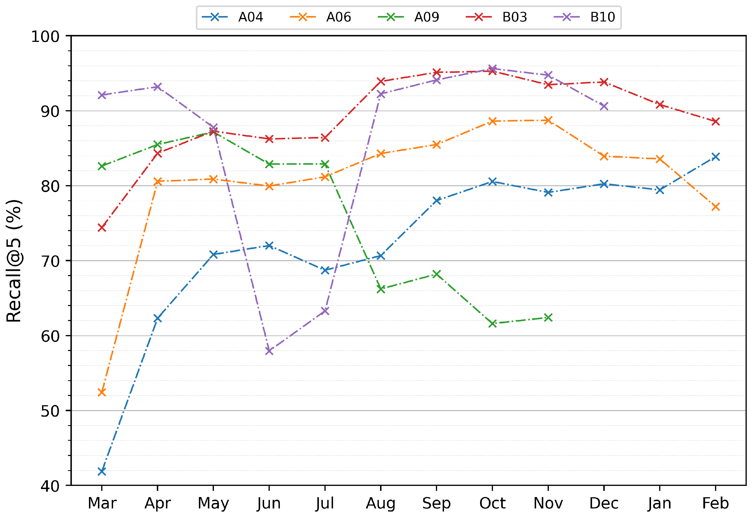
We made a test evaluation for each month using the previous months as training and validation data. We split randomly by 90% for training and 10% for validation. Figure 4, shows the Recall@5 results of our model over the entire user records. For each month, we tested the NAP model using the previous months as training samples. Therefore, when we tested at the end period of the user, we have the highest amount of training data. We picked the same 5 users from Figure 3 and each of them has different tendencies. Looking at A04, we see an expected behavior with a better test performance by having more training data. In B03 and A06, we also have an improvement over the months, but for the last months, we have a small decrease. A09 presents good performance for the first months but for the following months, it significantly decreases. B10 shows fluctuation along with the entire usage. It is essential to say that the top 5 most-used apps have a significant impact on performance. The considerable drop in the test results for A09 in August follows the most used top 5 apps percentage drop in Figure 3.
4.2. Overfitting Issue
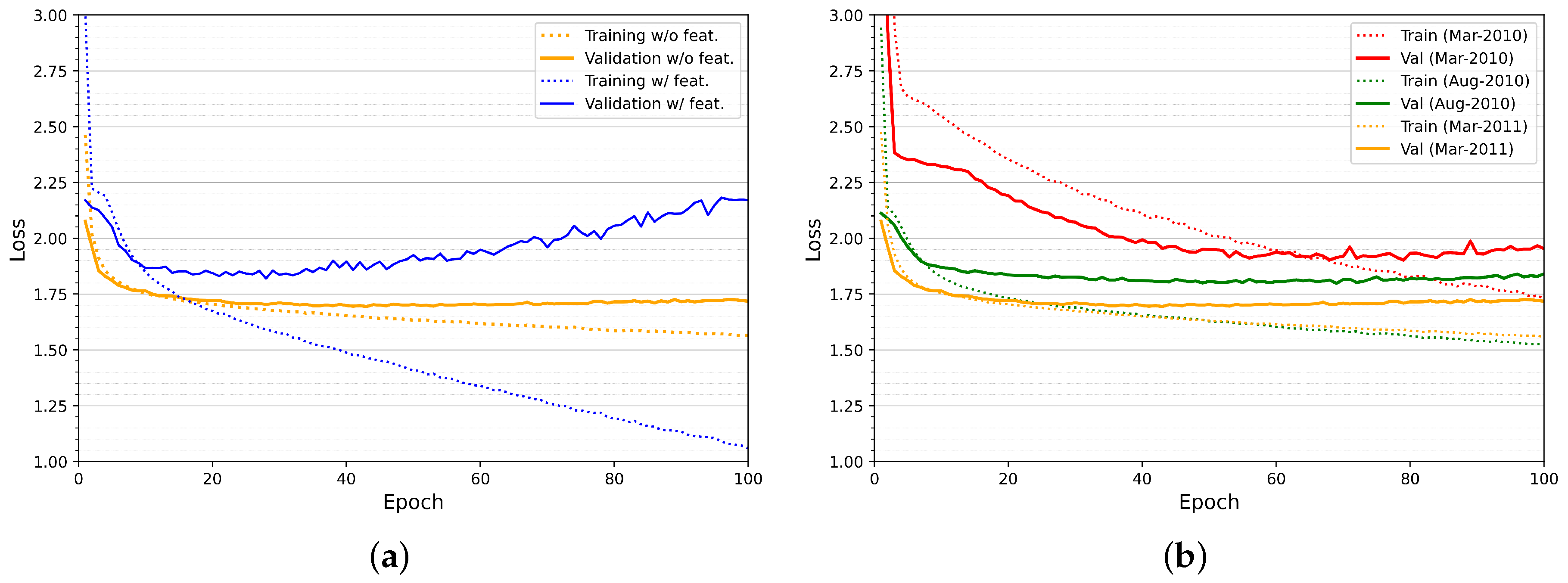
The overfitting was also stated in [13] when they used neural networks to app prediction. RNNs are powerful models; however, it overfits quickly [20]. When we consider the input, including the features and with small training data amount, we have a sharp growth in validation loss and a fast reduction in the training loss, configuring the overfitting, as presented in Figure 5a. If we reduce the complexity of the input, removing the features, the overfitting is significantly reduced. When we compare with the losses results from the subsequent months, we see a stabilization of the losses curve, since we have more training data, as shown in Figure 5b.
4.3. Performance Changing the Number of Previous Apps
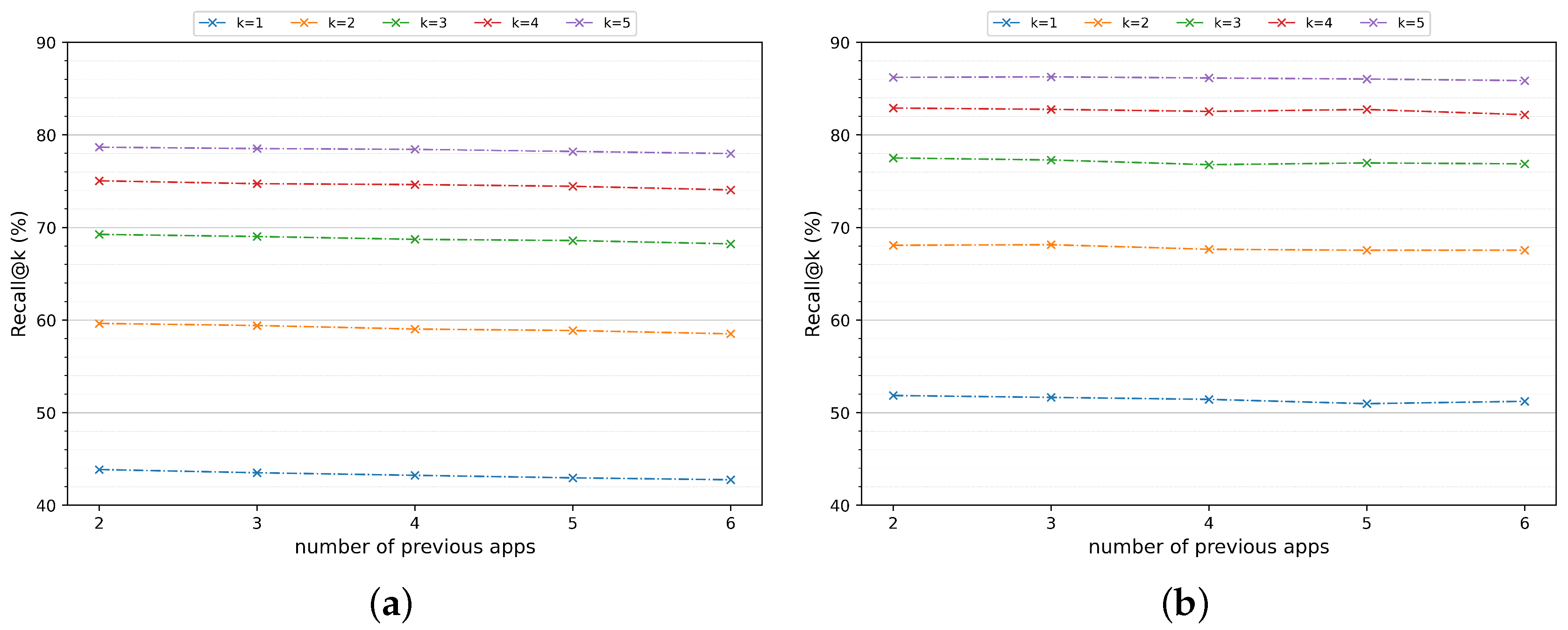
We also evaluate the results changing the number of previous applications. The results are shown in Figure 6. We changed from two previous applications until 6 and the performance slightly decreases in all Recall@k as we increase the previous applications. Figure 6a presents the results for all users where we evaluated all months and computed the average (except the first month). In Figure 6b, we computed the best month prediction results for all users. Looking at Recall@5, we have 78.90% from the left plot against 86.55% from the right. Usually, the prediction results for the first months are low, making a high amplitude between the average and maximum results. If we compare the Recall@5 from Figure 6a with the average of the last five months, we have an improvement from 78.90% to 80.30%. However, it is essential to keep in mind that some users presented the opposite behavior, as explored in Figure 4.
4.4. Impact of the Features
In [8] they used the same dataset, and they reported that the features did not provide significant improvement in their results. Using NAP with two previous apps and including the features, we had instead, a small reduction in the Recall@k results, as shown in Table 1. The results are the average of all users in all month tests.
The results show that the features might help during the training phase; however, it does not guarantee test results improvement, being evidence that the user changes his app usage behavior. If in one month we can infer the user usually plays games during the night, this argument might not be valid for the next month.
4.5. Comparison with Other Schemes
We compare our scheme with other schemes for the next app prediction:
- LRU: Refers to the least recently used items. The LRU selects the least recently used apps by each user;
- MFU: Refers to the most frequently used items. The MFU selects the most frequently used apps;
- AppUsage2Vec: The model developed using the app attention mechanism together with a dual deep neural network;
- FALCON: Model developed using cost-benefit adaptive prediction algorithm;
- APPM: Model based on PPM, which computes the conditional probability mapping of the characters in a sequence.
Two cached algorithms explored in the app prediction literature and also adopted by smartphone OS (Android) [21] are the Least Recently Used (LRU) and the Most Frequently Used (MFU). The LRU selects the least recently used apps by each user, and the MFU selects the most frequently used apps. Both LRU and MFU are updated continuously at each app record, and the test period is the same as it was used in NAP. Different from NAP, the LRU and MFU were updated during the test period.
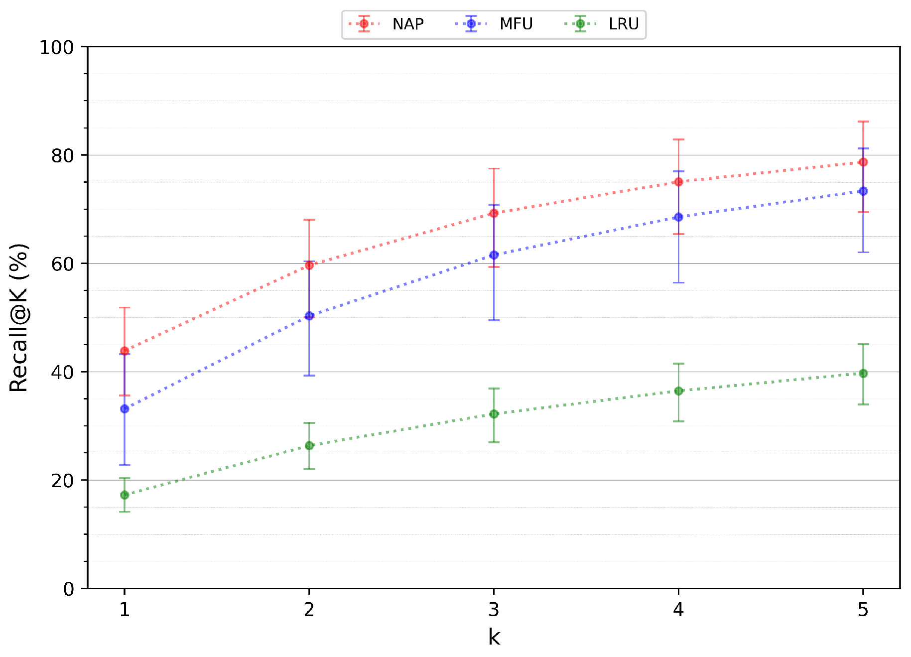
We tested the NAP with the standard LSTM and also with a bidirectional LSTM, which is an extension of traditional LSTMs that can improve model performance on sequence classification problems [22]. As expected, MFU had good results since we have shown the users concentrate their app usage in a few apps. The LRU presented poor performance, indicating the recently used apps might not be enough to represent the user patterns. The NAP performs better in all Recall@k tests as it is shown in Figure 7. The advantage of use NAP is the fact that it combines the essence of MFU and LRU, memorizing the most frequently apps and also accounting the previous apps used. We also implemented the AppUsage2Vec prediction model [13] due to their good results mentioned in their work. The model followed the same training and test arrangement as it was done using the NAP. Our model performed slightly better than the AppUsage2Vec, as shown in Table 2. The two works follow a similar structure, accounting for the previously used apps and using a neural network. The advantage of NAP is the fact that it is relatively simple to implement, and models based on RNN have been extensively explored in the literature for different types of sequence prediction tasks. We also compared with two other works stated in Section 2 since they have used the same dataset. FALCON provided the Recall@1,3,5, and APPM provided only the Recall@5, and NAP also has surpassed both of them.
5. Conclusions
Even though much work has been done in this decade, predicting the next application is still a difficult challenge since we have to deal with human behavior, which is contradictory in many ways. However, NAP proposed in this work shows a better model to describe the application usage. Unlike the related work, we proposed analyzing in detail month by month predictions to better understand the app prediction task’s complexity. We have shown that users can present chaotic application usage behavior and also tried to include different features and change the sequence length to see the impact on the performance. NAP shows that the few previous applications provided better performance compared to the higher number of previous applications. Unfortunately, the features did not improve the test results, and therefore, it reinforces some earlier works that also presented inexpressive improvement using the features. The results using NAP are relevant when compared with cited works. Consequently, it shows that we can transfer the knowledge acquired in language models to the application prediction task.
Author Contributions
Conceptualization, J.J., H.J. and G.S.M.; methodology, G.S.M. and J.J.; software, G.S.M.; validation, J.J. and H.J.; formal analysis, G.S.M.; investigation, G.S.M.; resources, J.J.; writing—original draft preparation, G.S.M.; writing—review and editing, G.S.M. and J.J.; supervision, J.J. and H.J. All authors have read and agreed to the published version of the manuscript.
Funding
This research was supported in part by Korea Institute for Advancement of Technology (KIAT) grant funded by the Korea Government (MOTIE) (N0001883, The Competency Development Program for Industry Specialist) and by MSIT (Ministry of Science and ICT), Korea, under the ICT Creative Consilience program (IITP-2020-0-01821) supervised by the IITP (Institute for Information & Communications Technology Planning & Evaluation).
Conflicts of Interest
The authors declare no conflict of interest. The funders had no role in the design of the study; in the collection, analyses, or interpretation of data; in the writing of the manuscript, or in the decision to publish the results.
Abbreviations
The following abbreviations are used in this manuscript:
| NAP | Natural App Processing |
| NLM | Neural Language Modeling |
| LM | Language Modeling |
| DNN | Deep Neural Network |
| RNN | Recurrent Neural Network |
| LSTM | Long Short Term Memory |
| LRU | Least Recently Used |
| MFU | Most Frequently Used |
| PPM | Prediction by Partial Match |
| APPM | App Prediction by Partial Match |
References
- Number of Available Applications in the Google Play Store from December 2009 to June 2019. Available online: https://www.statista.com/statistics/266210/number-of-available-applications-in-the-google-play-store/ (accessed on 3 July 2019).
- Liao, Z.X.; Li, S.C.; Peng, W.C.; Yu, P.S.; Liu, T.C. On the feature discovery for app usage prediction in smartphones. arXiv 2013, arXiv:1309.7982. [Google Scholar]
- Yan, T.; Chu, D.; Ganesan, D.; Kansal, A.; Liu, J. Fast app launching for mobile devices using predictive user context. MobiSys 2012, 113–126. [Google Scholar] [CrossRef]
- Li, C.; Bao, J.; Wang, H. Optimizing low memory killers for mobile devices using reinforcement learning. In Proceedings of the 2017 13th International Wireless Communications and Mobile Computing Conference (IWCMC), Valencia, Spain, 26–30 June 2017; pp. 2169–2174. [Google Scholar] [CrossRef]
- Time Series Forecasting. Available online: https://www.tensorflow.org/tutorials/structured_data/time_series (accessed on 1 August 2020).
- Yoav, G.; Graeme, H. Neural Network Methods in Natural Language Processing; Morgan & Claypool: San Rafael, SR, USA, 2017; pp. 104–113. [Google Scholar]
- Natarajan, N.; Shin, D.; Dhillon, I.S. Which app will you use next? collaborative filtering with interactional context. RecSys 2013, 201–208. [Google Scholar] [CrossRef]
- Parate, A.; Böhmer, M.; Chu, D.; Ganesan, D.; Marlin, B.M. Practical prediction and prefetch for faster access to applications on mobile phones. In Proceedings of the ACM International Joint Conference on Pervasive and Ubiquitous Computing, Zurich, Switzerland, 8–12 September 2013; pp. 275–284. [Google Scholar] [CrossRef] [Green Version]
- Cleary, J.; Witten, I. Data Compression Using Adaptive Coding and Partial String Matching. IEEE Trans. Commun. 1984, 32, 396–402. [Google Scholar] [CrossRef] [Green Version]
- Shepard, C.; Rahmati, A.; Tossell, C.; Zhong, L.; Kortum, P. LiveLab: Measuring wireless networks and smartphone users in the field. SIGMETRICS Perform. Eval. Rev. 2010, 38, 15–20. [Google Scholar] [CrossRef]
- Huang, K.; Zhang, C.; Ma, X.; Chen, G. Predicting mobile application usage using contextual information. In Proceedings of the ACM Conference on Ubiquitous Computing, Pittsburgh, PA, USA, 5–8 September 2012; pp. 1059–1065. [Google Scholar] [CrossRef] [Green Version]
- Xu, S.; Li, W.; Zhang, X.; Gao, S.; Zhan, T.; Zhao, Y.; Zhu, W.; Sun, T. Predicting Smartphone App Usage with Recurrent Neural Networks; Springer: Berlin, Germany, 2018; pp. 532–544. [Google Scholar] [CrossRef]
- Zhao, S.; Luo, Z.; Jiang, Z.; Wang, H.; Xu, F.; Li, S.; Yin, J.; Pan, G. AppUsage2Vec: Modeling Smartphone App Usage for Prediction. In Proceedings of the 2019 IEEE 35th International Conference on Data Engineering (ICDE), Macao, China, 8–11 April 2019; pp. 1322–1333. [Google Scholar] [CrossRef]
- Le, Q.V.; Mikolov, T. Distributed representations of sentences and documents. arXiv 2014, arXiv:1405.4053. [Google Scholar]
- Available online: https://www.tensorflow.org/tutorials/tensorflow_text/intro (accessed on 1 August 2020).
- Mikolov, T.; Sutskever, I.; Chen, K.; Corrado, G.; Dean, J. Distributed Representations of Words and Phrases and Their Compositionality. Adv. Neural Inf. Process. Syst. 2013, 2, 3111–3119. [Google Scholar] [CrossRef]
- Hochreiter, S. The Vanishing Gradient Problem During Learning Recurrent Neural Nets and Problem Solutions. Int. J. Uncertain. Fuzziness Knowl.-Based Syst. 1998, 6, 107–116. [Google Scholar] [CrossRef] [Green Version]
- Many-to-One RNN. Available online: https://stanford.edu/~shervine/teaching/cs-230/cheatsheet-recurrent-neural-networks (accessed on 1 August 2020).
- Hochreiter, S.; Schmidhuber, J. Long Short-Term Memory. Neural Comput. 1997, 9, 1735–1780. [Google Scholar] [CrossRef] [PubMed]
- Gal, Y.; Ghahramani, Z. A Theoretically Grounded Application of Dropout in Recurrent Neural Networks. Adv. Neural Inf. Process. Syst. 2016, 1027–1035. [Google Scholar] [CrossRef]
- LruCache. Available online: https://developer.android.com/reference/android/util/LruCache (accessed on 1 August 2020).
- Graves, A.; Schmidhuber, J. Framewise phoneme classification with bidirectional LSTM networks. In Proceedings of the 2005 IEEE International Joint Conference on Neural Networks, Montreal, QC, Canada, 31 July–4 August 2005; Volume 4, pp. 2047–2052. [Google Scholar] [CrossRef] [Green Version]
Figure 1.
Summary of the Natural App Processing (NAP) approach for app prediction task.

Figure 2.
Feedforward propagation diagram in many-to-one recurrent neural network (RNN).

Figure 3.
Top five apps usage percentage from June to October.

Figure 4.
Recall@5 for each month for five users’ results using the NAP model.

Figure 5.
Cross-entropy loss for B09 user including and not including the features (a) and cross-entropy loss for B09 in different months not including the features (b).
Figure 5.
Cross-entropy loss for B09 user including and not including the features (a) and cross-entropy loss for B09 in different months not including the features (b).

Figure 6.
Recall@k performance average (a) and best month performance (b) for all users.

Figure 7.
Recall@k performance for NAP, LRU and MFU.


Table 1.
Recall@k comparison results using the features and without the features.
| NAP | Recall@1 | Recall@2 | Recall@3 | Recall@4 | Recall@5 |
|---|---|---|---|---|---|
| No features | 42.79% | 59.67% | 69.40% | 75.20% | 78.90% |
| With features | 40.36% | 57.18% | 66.93% | 73.11% | 77.13% |
Table 2.
Best month Recall@k results for each model.
| Model | Recall@1 | Recall@2 | Recall@3 | Recall@4 | Recall@5 |
|---|---|---|---|---|---|
| NAP (Bidirectional) | 50.79% | 68.14% | 77.65% | 83.00% | 86.55% |
| NAP | 50.59% | 68.02% | 77.51% | 82.98% | 86.42% |
| AppUsage2Vec | 49.99% | 67.41% | 76.78% | 82.67% | 85.93% |
| APPM | - | - | - | - | 81.35% |
| FALCON | 50.0% | - | 79.0% | - | 80.0% |
| MFU | 43.24% | 60.37% | 70.84% | 76.98% | 81.22% |
| LRU | 20.34% | 30.60% | 36.86% | 41.50% | 45.08% |
© 2020 by the authors. Licensee MDPI, Basel, Switzerland. This article is an open access article distributed under the terms and conditions of the Creative Commons Attribution (CC BY) license (http://creativecommons.org/licenses/by/4.0/).
Share and Cite
MDPI and ACS Style
Moreira, G.S.; Jo, H.; Jeong, J. NAP: Natural App Processing for Predictive User Contexts in Mobile Smartphones. Appl. Sci. 2020, 10, 6657. https://0-doi-org.brum.beds.ac.uk/10.3390/app10196657
AMA Style
Moreira GS, Jo H, Jeong J. NAP: Natural App Processing for Predictive User Contexts in Mobile Smartphones. Applied Sciences. 2020; 10(19):6657. https://0-doi-org.brum.beds.ac.uk/10.3390/app10196657
Chicago/Turabian StyleMoreira, Gabriel S., Heeseung Jo, and Jinkyu Jeong. 2020. "NAP: Natural App Processing for Predictive User Contexts in Mobile Smartphones" Applied Sciences 10, no. 19: 6657. https://0-doi-org.brum.beds.ac.uk/10.3390/app10196657
Note that from the first issue of 2016, this journal uses article numbers instead of page numbers. See further details here.