Empowering Predictive Maintenance: A Hybrid Method to Diagnose Abnormal Situations

Featured Application

The proposed hybrid method may achieve a better performance than a single algorithm in any fault classification problem.

Abstract

Aerospace systems are composed of hundreds or thousands of components and complex subsystems which need an appropriate health monitoring capability to enable safe operation in various conditions. In terms of monitoring systems, it is possible to find a considerable number of state-of-the-art works in the literature related to ad-hoc solutions. Still, it is challenging to reuse them even with subtle differences in analogous subsystems or components. This paper proposes the Generic Anomaly Detection Hybridization Algorithm (GADHA) aiming to build a more reusable algorithm to support anomaly detection. The solution consists of analyzing different supervised machine learning classification algorithms combined in ensemble techniques, with a physical model when available, and two levels of a decision to estimate the current state of the monitored system. Finally, the proposed algorithm assures at least equal, or, more typically, better, overall accuracy in fault detection and isolation than the application of such algorithms alone, through few adaptations.

1. Introduction

In the field of Prognostics and Health Management (PHM), the key is to be capable of predicting the Remaining Useful Life (RUL) of a system. Even knowing that it is possible to establish prognostics without identifying the root cause, the understanding of the way the system is degrading gives an advantage in terms of health monitoring system development. Knowing the physical phenomena allows us to introduce a degrading model to support the data acquired during system utilization and better tuning the algorithms in charge of fault detection [1].

Without the degrading model, it is also possible to use statistics to learn the degradation behavior of a system of interest. Still, it would be necessary to have data available in many different situations. The data-driven approach, in this case, could manage the lack of the physics-model, but an anomaly may not be satisfactory classified.

To have both approaches helps in troubleshooting and also in predictive maintenance of assets. The recent development of the PHM field brought a series of new information to support maintainers in the task of identifying/isolating the root causes of a specific failure The hybrid approach, using both model-based (physics model) and data-driven (collected data during operation) approaches, enhances a health monitoring system to accomplish the goal of detecting faults and generating alerts [1,2].

Since predictive maintenance makes use of fault detection to help RUL prediction, the goal is to establish in advance the discovery of a faulty condition on the target system. The earlier the detection, the more time to plan resource allocation and schedule maintenance tasks [3]. The process to detect the fault and identify its root cause is called Fault-Detection and Isolation (FDI) [4]. An anomalous behavior is not necessarily a fault, and the present work uses an FDI method to establish a classification algorithm. The approach is capable of distinguishing faults from abnormal behaviors that are not faulty conditions of the system but can produce a system degradation and also impact the system’s RUL.

The FDI method makes use of sensory data that can bring noise, bias and sensor calibration problems [3]. Because each system has its characteristics, it is hard to develop a solution that can be widely adopted. The typical approach is to have algorithms adapted for each new case, even if the system is similar to another one that already has an implemented solution. If the system is not installed in the same way, with the same conditions, it is possible to have different noise and environment conditions that give different readings to the sensor.

The present work is an attempt to help the reuse of an FDI infrastructure and is the initial result of a hybrid approach called the Generic Anomaly Detection Hybridization Algorithm (GADHA). The next section will provide a literature review of solutions in the FDI field using hybrid methods. Then, the Material and Methods section describes the GADHA approach, and the results section shows the results achieved in a study case of fault detection and isolation on a spring-mass system. The discussion section brings the main achievements, and a brief conclusion section provides the main contributions of the work.

2. Literature Review

In a literature review about Fault Detection and Isolation, it was observed that most of the current solutions were very specific for a closed system or even a particular situation. It means that it is hard to reuse the solution. Even for a similar system, with a few different parameters, it would be necessary to implement adaptations. However, a minimal generalization becomes a difficult task.

The aeronautical industry was not completely unaware of this and had some initiatives to provide frameworks and recommendations that any customer, manufacturer, or stakeholder could adopt if desired. Even so, different protocols and standards were adopted depending mostly on the region (America or Europe) and segment (commercial or military). Nevertheless, two relevant frameworks provide significant levels of protocols in different layers to standardize implementations, products, communications, interface, processes, projects, and other subjects of interest.

The first and more comprehensive one is the Integrated Vehicle Health Management (IVHM). The National Aeronautics and Space Administration (NASA) was the first one to adopt and implement this concept. Nowadays, it has strong support from the Society of Automotive Engineers (SAE), and it was taken in different stages in the aviation industry [5,6,7].

The second initiative comes from the Machinery Information Management Open Systems Alliance (MIMOSA). Its proposed standards, namely Open System Architecture for Condition-Based Maintenance (OSA-CBM) and Open System Architecture for Enterprise Application Integration (OSA-EAI), have established protocols to support asset management [8].

The OSA-CBM framework is based on six layers depicted in Figure 1. From layers 1 to 3, the data flow is considering each component as an independent system, and its primary concern is to best estimate the actual state for the given parts. From layers 4 to 6, a gradual increment on data fusion takes place to raise awareness of the whole monitored system situation. In the end, it is up to the responsible manager to evaluate and decide the actions or inaction that will be applied to the respective system, restarting the cycle again.

It is essential to highlight that diagnosis takes place mostly at layer 4, starting in layer 3, while the system is being operated in the OSA-CBM framework. In terms of asset management, it would be necessary to establish the history of the system operation and also previous knowledge in the system’s reliability. Such capability is acquired from the use of the OSA-EAI framework and IVHM state-of-the-art implementations.

All those initiatives become crucial in an age of interoperable systems, and still more challenging because an Air Force, or an air transportation company, manages many different aircraft fleets, from varied manufacturers, for several environments and purposes. On the other hand, systems that apply the same protocol, standard architecture, and user interfaces in the same situation are simpler to support, since they can share a set of standard solutions and even components in some cases.

The term anomaly detection refers to the capability to identify anomalies based on the acquired data through pattern recognition that does not conform to the expected system behavior [9]. From all circumstances exposed so far in the anomaly detection and diagnosis fields, it is pronounced the number of anomaly detection algorithms and methodologies aimed at ad-hoc solutions. The best way to analyze this argument is by dividing those studies into three main approaches:

• Data-Driven techniques: It is independent of a physical model, and it uses the historical records and online data to solve anomaly detection problems. The system or component is irrelevant from this perspective, and generalization can only be considered if data-sets are the same in all aspects;
• Model-Based techniques: It has sets of equations that explain mostly the behavior of a physical system. The data are analyzed through these equations. Such models need to be as representative as possible to the system, but this rarely happens due to noise, lack of complete knowledge of phenomenons involved, disturbances, and even impossibility to perform the necessary measurements;
• Hybrid techniques: It is the combination of the other two techniques with their benefits and limitations. However, there are different ways to perform hybridization. So by abstracting the data-set and model, it is possible to extract the interaction architecture between both algorithms and check the feasibility and compatibility with the proposed system.

Hybrid approaches are taking place more often once data-driven techniques can explain part of that uncontrolled behavior presented in model-based approaches. The assumption that such methods could never reach a perfect representation in the real world is very plausible, and it leads to the assumption that more optimization is always possible. Although, it can be unnecessary if requirements do not demand it.

The concept of the wisdom of the crowd from statistics is interpreted in machine learning as Ensemble Learning. Considering a choice for one of the available algorithms in the literature, instead of training and applying only one instance of it, a considerable number of inducers are created and trained to obtain various countable results from different approaches. The work [10], in their survey about ensemble learning, points out the premise that the combination of multiple models compensates the error of a single inducer.

From this perspective, the present work was developed looking to generate a framework to support fault classification with a hybrid approach. The model-based capability to establish the basic behavior of the system will be combined with ensemble techniques that can mix a set of different data-driven methods, depending on the system characteristics.

Varied methods to organize them can be found in the literature, and this is one of the most relevant aspects observed for this work. It addresses the ability of ensemble learning in generalizing many different fashion distinct algorithms or even different versions of one of them. Besides the fact of their straightforward application, they provided the necessary hint to tackle the research problem in this study.

Ensemble learning is a broad term in machine learning used for the combination of multiples inducers to make a decision. Thereby, the primary purpose of this technique is to try to use several inducers to compensate for the errors of one or a few of them [10].

There are three major approaches for ensemble methods: boosting, bagging, and stacking. All the others can be considered derivations, adaptations, or a mix of them.

Table 1. Ensemble methods meta-algorithms.

Meta-Algorithm	Inducers	Description
Boosting	Often homogeneous	A model depends on the previous one
Bagging	Often homogeneous	Independent weak learns, they can be trained in parallel
Stacking	Often heterogeneous	Independent weak learns, they can be trained in parallel

resumes these meta-algorithms used in [11,12,13].

Ensemble methods have been used to handle FDI problems in several publications. The work [13] did research comparing different machine learning classifiers, and the best results were achieved using ensemble techniques to detect submersible electrical pump failures. The work [12] developed an ensemble of dynamic neural networks for FDI from gas turbine engines. His approach claims to be the first one to use ensemble methods through system identification to generate residuals instead of evaluating them like previous works. In the time of paper writing, ensembles can be considered as the state-of-the-art technique for a broad set of machine learning and real-life challenges [10].

Adaptative Neuro-Fuzzy Inference System (ANFIS) aggregates the Artificial Neural Networks (ANN) concept of robustness, adaptation, non-linear mapping, and at the same time as it is based on the Takagi–Sugeno–Kang inference model [14]. The Fuzzy Inference System (FIS), or fuzzy logic, can handle uncertainties and imprecise pieces of information. While FIS requires excellent knowledge to have an appropriate set of rules to achieve better accuracy, ANFIS does not demand an expert since it inherits the learning ability from ANN. It means that ANFIS can shape its rules through training algorithms as back-propagation applied to ANN.

ANFIS have been applied in many recent works to FDI, e.g., [14,15,16]. All of them are in an ad-hoc approach since such works have used ANFIS straightforwardly to analyze system output data. However, it is not necessary to generalize ANFIS in an FDI perspective if other methods handle system output variables. Reference [17] has applied fuzzy decision making for component selection. From this perspective, it is analog that the decisions taken from previous methods can be analyzed as such components to make a final decision.

Some model-based techniques typically depend on other methods since they are thoroughly focused on residuals generations. Reference [18] is a good example of such a case where a Support Vector Machine (SVM) and Consistency-Based Fault Isolation (CBFI) are employed to perform an evaluation. In brief, CBFI compares the residuals with some subsets of faults that can “explain” the residuals.

Three works [1,18,19] employ structural analysis as their physical model to generate residuals. The main differences lie in the choices of data-driven algorithms that select the best residual generators and system where they are applicable. Although [1,18] can be applied for any complex system, all structural analyses require a thorough knowledge of the physical phenomena involved in such a system so that the greatest number of algebraic equations can be included into the model.

Ref. [20] combined a state observer and an ANN to detect and isolate small faults of actuators in closed-loop control systems. The role of the ANN is to analyze residuals, and the model-based classification results in the decision reasoning process. Therefore, it does not involve interaction between techniques since one does not affect others.

The work [21] proposed a hybrid approach to control and detect anomalies for fuel cell stack cooling control. They employed Active Disturbance Rejection Control (ADRC), a data-driven technique, to estimate uncertainty and evaluate residuals to a Proportional Integral Derivative (PID) control. The Extended State Observer (ESO) represents the physical model responsible for the residual generation. The interaction between ADRC and ESO inside a closed loop promotes a great synergy. Finally, the work [22] conducted a dedicated study about model-based and data-driven fusion approaches to FDI.

3. Method

The proposed method is a heuristic solution that combines different supervised machine learning techniques and an optional physical model to classify abnormal situations in complex systems. The abnormal situation (or anomaly) may be a system degradation, a fault or an operational deviation. For this reason, it was named Generic Anomaly Detection Hybridization Algorithm (GADHA). The detection method can be used in conjunction with Health Assessment and Prognostic Assessment techniques to determine the remaining useful life (RUL) of the equipment and thus to assist Condition-Based Maintenance implementation.

3.1. General Method Description

Figure 2 shows the general concept of GADHA. It is divided into four processes stages that are based on the OSA-CBM framework. The first two stages have the same name and functionalities of OSA-CBM layers of Data Acquisition and Data Manipulation. The two last stages of GADHA (First Instance Classification and Final Instance Classification) performs OSA-CBM State Detection layer, combining data-driven and model-based detection. Each process stage is composed of one or many activities, as identified and detailed in Figure 2.

The output of GADHA corresponds to the system state detection. If the detected state is an abnormal condition, it may correspond to an incipient system failure or an abnormal operating condition. The abnormal condition is then associated with a particular equipment degradation (Health Assessment). Finally, based on the equipment failure mechanism and the expected equipment operational condition, one can estimate the system Prognostic Assessment (RUL).

3.2. Method Detailed Description

The steps of GADHA, as exhibited in Figure 2, are detailed in the following sections. The activities are labeled only by numbers and the title of the main process to reduce words on the figure.

3.2.1. Data-Acquisition

Data acquisition process is the process of measuring sensor data and transforming analogical data into digital information. The details and main challenges associated with this process is out of the scope of this work. This process is composed only by Activity 1 (Raw Data Acquisition), as exhibited in Figure 2.

3.2.2. Data Manipulation

Data Manipulation step can be performed either by a data-driven pre-processing (Activity 2) or by a model-based pre-processing (Activity 3). On each activity, data manipulation goal is either to reduce input data dimensionality or to transform input data using filters on a data cleaning approach.

Activity 2—Data-Driven Pre-Processing

When data-driven pre-processing techniques are used to reduce input data dimensionality, it is done without any knowledge about the system design or behavior, and it is also called data-driven feature extraction.

Linear Discriminant Analysis (LDA) is often used as a data-driven pre-processing step to reduce the dimensionality of input data in classification tasks, which also demands a supervised training. This approach looks for the component axes that maximize data variance; likewise, for axes that maximize multiple class separation. However, there are many cases where LDA is the classification algorithm due to all those characteristics [23]. The analyst may choose several other different techniques to reduce the dimensionality of input data based on feature extraction techniques that do not depend on the specialized knowledge about the system.

When data-driven pre-processing techniques are used to filter input data, on a data cleaning approach, it is done by implementing filters that do not depend on any knowledge about the system. For instance, winsorizing transformations is often used to reduce the effect of possible spurious outliers.

3.2.3. First Instance Classification

In this stage, GADHA counts with ensemble techniques and with the physical model to predict the state-condition of the system. It is necessary to thoroughly estimate the initial state parameters of the physical model once the behavior of the system is an outgrowth of them.

There are scenarios where the position measurement is straightforward, and the estimation of those initial values becomes a noise reduction issue. However, there is one scenario that only provides accelerometer and gyroscope measurements. In this case, the estimation becomes more laborious and requires more steps. Thus, it will demonstrate the data-driven methods responsible for estimating the release height, when just acceleration is available.

Activity 3—Model-Based Pre-Processing

When model-based pre-processing techniques are used to reduce input data dimensionality, it is done based on specialized knowledge about the system design or behavior, and it is also called model-based feature extraction. This technical knowledge is expressed either by a set of rules to determine if a particular feature is present or not or by the definition of acceptable thresholds based on system noise modeling. When model-based pre-processing techniques are used to filter input data, on a data cleaning approach, it is done by implementing filters based on the system noise and expected behavioral characteristics.

Activities 2 and 3 are not mutually exclusive and can be performed in conjunction to reduce input data dimensionality (features extraction) or to filter input data. This means that if one wishes to create an embracing number of extracted features, he may consists ofder features extracted by either data-driven pre-processing or by model-based pre-processing. Furthemore, the data cleaning approach may encompass both data-driven filters as well as model-based filters.

Activity 4—Ensemble Learning Classification (Data-Driven)

The ensemble learning classification performed on Activity 4 of GADHA receives as inputs all features extracted from Activities 2 and 3, and classify system state, estimating what is the most probable state among a finite and enumerable list of possible system states.

To perform this classification, initially, ensembles shall be created considering sets of machine learning inducers. Each ensemble groups a certain number of inducers, and each inducer attempts to estimate system state based on input data. The final classification of each ensemble corresponds to the best estimate considering the ensemble inducers estimates as well as the performance metrics of each inducer. In the scope of this work, the final classification of each ensemble is called the committee classification technique.

Inducers or learners are machine learning algorithms in the scope of this work. They are split into two categories: parametric and non-parametric, depending if the algorithm is parametric or not. Support Vector Machine (SVM) and Decision-Tree (DT) are examples of machine learning non-parametric algorithms, while Artificial Neural Network (ANN) and Naive Bayes (NB) are examples of parametric inducers.

At GADHA, it is proposed the usage of ensembles composed of three inducers for simplicity because even values are more prone to draws, and three is the smallest non-unit positive odd value of ensemble inducers quantity. These three inducers ensembles are called Ensemble Triads (ET).

Based on the above definitions, Ensemble Triads can be classified as Heterogeneous ET, Homogeneous non-parametric ET, or Homogeneous parametric ET. Figure 3 shows the ET general concept.

According to GADHA, the Ensemble Learning Classification activity is performed based on several ETs of different types (heterogeneous, homogeneous non-parametric, homogeneous parametric), built randomly according to the following hyperparameters: number of triads to build, set of parametric algorithms, set of non-parametric algorithms and proportion of heterogeneous, homogeneous non-parametric, and homogeneous parametric ET to build, expressed by the proportions ${\lambda }_1,{\lambda }_2$, and ${\lambda }_3$.

Table 2. Ensemble Triads hyperparameters.

Hyperparameter	Default Value	Description
N	1000	Number of triads to build
${\Theta }^i$	{∅}	Set of parametric functions
${\Gamma }^j$	{∅}	Set of non-parametric functions
$\Lambda$	$\{{\lambda }_1{\lambda }_2{\lambda }_3\}$	Set of proportions among the three main triads set, being that ${\lambda }_1+{\lambda }_2+{\lambda }_3=1$
${\lambda }_1$	0.5	Heterogeneous triads proportion
${\lambda }_2$	0.25	Homogeneous non-parametric triads proportion
${\lambda }_3$	0.25	Homogeneous parametric triads proportion

illustrates the Ensemble Triads hyperparameters.

According to GADHA notation, the set $\Gamma$ corresponds to the set of non-parametric functions $\gamma (\overrightarrow{v})$, and the set $\Theta$ is the set of parametric functions $\theta (\overrightarrow{v})$. The feature space $\overrightarrow{V^{\iota }}$ may have three different dimensions depending on which data acquisition is made from sensors. The function argument $\overrightarrow{v}$ is a vector that can be any subspace feature, defined in Equation (1).

$$\begin{array}{c}\hfill {\Theta }^i=\{{\theta }_1({\overrightarrow{v}}_1),\dots ,{\theta }_i({\overrightarrow{v}}_i)|{\overrightarrow{v}}_i\subset {\overrightarrow{V}}^{\iota },{\overrightarrow{v}}_1\ne {\overrightarrow{v}}_i,i\in \mathbb{N}andi>1\};\\ \hfill {\Gamma }^j=\{{\gamma }_1({\overrightarrow{v}}_1),\dots ,{\gamma }_j({\overrightarrow{v}}_j)|{\overrightarrow{v}}_j\subset {\overrightarrow{V}}^{\iota },j\in \mathbb{N}andj>1\};\end{array}$$

(1)

The value of $\iota$ indicates the same dimensions for both sets. It is not a hyper-parameter of the algorithm, but the sum up of all declared functions inside any category. One example of possible functions for $\Theta$ or $\Gamma$ can be visualized in Equation (2). In the example of Equation (2), parametric functions are Artificial Neural Networks (ANN) and Naive Bayes (NB), while non-parametric functions are Support Vector Machine (SVM) and Decision Tree (DT). The analyst may choose other parametric and/or non-parametric functions as, for instance, Linear Discriminant Analysis (LDA), as done on the case study of this work.

$$\begin{array}{c}\hfill {\Theta }^i=\{ANN,NB\},i=2\\ \hfill {\Gamma }^j=\{SVM,DT\},j=2\end{array}$$

(2)

For the heterogeneous ensemble triads, the same input data are used for all inducers. Each inducer of each heterogeneous ET will receive as input the same subset of features extracted on Activities 2 and 3 of GADHA. The input vector consumed by each inducer is a subset of all features vector and is called the Input Feature Vector. Therefore, the heterogeneous ET has only one Input Feature Vector consumed by all inducers.

On the other hand, for the homogeneous ensemble triads, whether the ET is parametric or not, different input vectors are used for different inducers, once the same inducer would be prone to perform the same classification when subjected to the same data. This means that each inducer of each homogeneous ET will receive as input a different subset of features extracted on Activities 2 and 3 of GADHA. The input vector consumed by each inducer is a subset of all features vector and is called the Input Feature Vector. Therefore, the homogeneous ET has three different Input Feature Vectors, one for each inducer.

The final classification of each ensemble (Committee Classification Technique) considers both the ensemble inducers estimates and the performance metrics of each inducer. A particular case of this committee classification technique corresponds to the majority voting, where the performance metric of the inducers will only be taken into account to select the best performance inducer if each ET inducer provides a different classification.

The inducers performance metrics correspond to true-positives (TP), false-positives (FP), true-negatives (TN), false-negatives (FN), precision (PCS), recall (RCA), F1-score (F1), and accuracy (ACC).

Table 3. Machine Learning algorithms performance metrics.

Metric	Equation
TP	$T{P}_i=C_{i,i}$
TN	$T{N}_i={\sum }_{i=1}^n{\sum }_{j=1}^n{C}_{i,j}-{\sum }_{j=1}^n{C}_{i,j\ne i}-{\sum }_{j=1}^n{C}_{j,i\ne j}$
FP	$F{P}_i={\sum }_{j=1}^n{C}_{i,j\ne i}$
FN	$F{N}_i={\sum }_{j=1}^n{C}_{j,i}\ne j$
PCS	$PC{S}_i=\frac{T{P}_i}{T{P}_i+F{P}_i}$
RCA	$RC{A}_i=\frac{T{P}_i}{T{P}_i+F{N}_i}$
F1	$F{1}_i=\frac{PC{S}_i·RCAi}{PC{S}_i+RCAi}$
ACC	$ACC=\frac{TP+TN}{TP+TN+FP+FN}$

summarizes all of them according to a confusion matrix $C_{n,n}$, true values represented by columns, predict values by rows, and n is the number of rows and columns, respectively. These equations and definitions also can be found in [12,13,24].

At the end of the committee classification, it will be associated with a single system state classification per ensemble triad. Each ensemble triad is defined in performance metrics such as the inducer’s metrics according to Table 3. If ensemble triad performance is below a minimum threshold, then the state classification associated with the ET is considered as under suspect, which means that ET was not able to make a consistent decision.

Finally, taking into consideration all ensemble triads, it is possible to create a vector that can express overall ET classification performance for each possible system state. This vector is represented by ${\overrightarrow{d}}^{s+1}$, where s is the total system possible states. The first s elements of this vector correspond to the percentage of ensemble triads that classified the system state corresponding to the vector element. The element $s+1$ corresponds to the percentage of triads that were not able to make a consistent decision (undefined state), according to the criteria defined previously.

All triad decisions have the same influence, and they have counted as votes for each state n such a manner that lack of decisions take count. The votes received by each state are held in ${\sigma }_i$, while $\xi$ holds the total number of no-decisions. Thus, the vector elements from $y_1$ to $y_s$ (inclusive) are the respective state votes proportion, while the element $y_{s+1}$ is the undefined state votes proportion.

$$\begin{array}{c}\hfill {\overrightarrow{d}}^{s+1}=\{y_1,y_2,\dots ,y_s,y_{s+1}\}|{\Sigma }_{i=1}^{s+1}{y}_i=1,0\le y_i\le 1\\ \hfill y_i=\left\{\begin{array}{ccc}\hfill \frac{{\sigma }_i}{N}& \mathrm{for}& i\le s\hfill \\ \hfill \frac{\xi }{N}& \mathrm{for}& i=s+1\hfill \end{array}\right.\end{array}$$

(3)

Activity 5—Residues Estimation Based on Physical Models

The ensemble learning classification performed on Activity 4 of GADHA receives as inputs all features extracted from Activities 2 and 3, and classify system state, estimating what is the most probable state among a finite and enumerable list of possible system states.

Residues estimation is made by comparing real system state values with expected values of each system state estimated by the respective physical model. This comparison is made straightforwardly, subtracting one value from the other.

Physical models are typically achieved through dynamic equations and state variables, but can also be represented in different ways, using, for instance, lookup tables.

In the case study of this work, the physical model is a linear system representing a generic three degree of freedom mass-spring-damper model. Such a model is suitable to represent many aircraft landing-gear part numbers.

Activity 6—Ensemble Learning Classification (Model-Based)

The ensemble learning classification performed on Activity 6 of GADHA is the same process as described on Activity 4, except by the fact that the inputs of this process are the residues estimated on Activity 5. Therefore, residues correspond to features to be used for system state classification on each ET.

3.2.4. Final Instance Classification

The final instance classification is a process made of two activities: Decision Reasoning (Activity 7) and State Detection (Activity 8).

Activity 7—Decision Reasoning

Decision Reasoning receives vector ${\overrightarrow{d}}^{s+1}$ from both data-driven and model-based ET (activities 4 and 6 respectively). Alternatively, instead of receiving the output of activity 6, the Decision Reasoning process can receive the residues values vector directly from Activity 5, as shown in Figure 2.

As an output, the Decision Reasoning process delivers to the next activity a harmonized decision vector ${\overrightarrow{d}}^{s+1}$, considering both data-driven and model-based preliminary results. This task can be performed considering either a linear combination of model-based and data-driven decision vectors or a revisiting process of the ET results, applying, for instance, ANFIS (Artificial Network Fuzzy Inference System) algorithm to estimate system state.

If an algorithm is used to estimate system state directly from the output of Activities 4, 5 and 6, as for instance ANFIS, then Activity 7 and Activity 8 are merged on a single activity that is able to provide system state detection.

Activity 8—State Detection

The State Detection process selects the most probable state from the harmonized decision vector and informs it to the end-user, also estimating the confidence level of this estimate. As highlighted before, data fusion algorithms as ANFIS can also be used on this task, as detailed in the sequence.

ANFIS Semantic Aspects

One of the best strengths of the Fuzzy Inference System (FIS) is its capability to handle subject measurements [6], and this is the main reason to choose it as a manager—its decision is based on its staff. In this method, the physical model, ET₁, and ET₂ are their staff whose opinions are expressed through vector ${\overrightarrow{d}}^{s+1}$.

The Membership Function (MF) performs the fuzzification step [25]. This technique defines two sets of Gaussian MF, both with the same size, where ${\mathsf{\Omega }}_1=$ Eliminated, Candidate, Winner corresponds to the system-state estimated and ${\mathsf{\Omega }}_2=$ Negligible, Acceptable, Unacceptable corresponds to the indecision degrees.

Considering those same vectors from a semantic perspective, it is possible to make the sentences described in

Table 4. Semantic perspective.

Sentence
$d_{1,1}$ is an eliminated system-state
$d_{1,2}$ is a candidate system-state
$d_{1,3}$ is a candidate system-state
$d_{1,4}$ is an acceptable indecision grade
$d_{2,1}$ is an eliminated system-state
$d_{2,2}$ is a candidate system-state
$d_{2,3}$ is a candidate system-state
$d_{2,4}$ is an acceptable indecision grade
$d_{3,1}$ is a eliminated system-state
$d_{3,2}$ is a candidate system-state
$d_{3,3}$ is a winner system-state
$d_{3,4}$ is a negligible indecision grade

. Different types of membership functions can be used to support the fuzzification process.

On Table 4, $d_{i,j}$ corresponds to the result vector of first instance classification algorithm, where index i corresponds to the vector origin (physical model, ET₁, and ET₂), while index j corresponds to the system state under analysis. If the system has s states, j varies from 1 to $s+1$, where $s+1$ corresponds to undefined state (indecision grade).

Table 4 can be very assertive when one of its elements declares a winner or an eliminated system-state. At the same time, it can be very subjective when declaring a candidate. It is not necessary to relate all system-states among each other since the MFs can provide a certain level of mutual-exclusivity when the sentences are considered assertive. It impacts the number of necessary rules that defines the size of 2nd, 3rd, and 4th layers. So, the set of useful rules for this methodology is the combination of correspondents system-states and correspondents indecision degree, as seen in Figure 4.

ANFIS Learning Algorithm

The ANFIS training makes use of Minimum Square (MS) to set its linear parameter in 4th layer and gradient descent (GD) algorithm to train its non-linear parameters in 1st layer. Primarily, it is performed a forward phase where non-linear parameters are kept fixed. After the 3rd layer processes its outputs, the linear parameters are calculated through MS, and the error is calculated when the 5th layer outputs its value. After that, the backward phase takes place and propagates the error to the 1st layer, where the MF parameters are adjusted. The learning algorithm applied in this technique can be visualized with more details in the following works: [26,27].

4. Case Study

The primary purpose of this study case is not about a landing-gear (LNG) development, but it is about how the actual state of a common landing-gear can be, as much as possible, correctly estimated. However, this specific component was selected to evaluate the proposed method accuracy in a more concrete case.

4.1. Physical Model

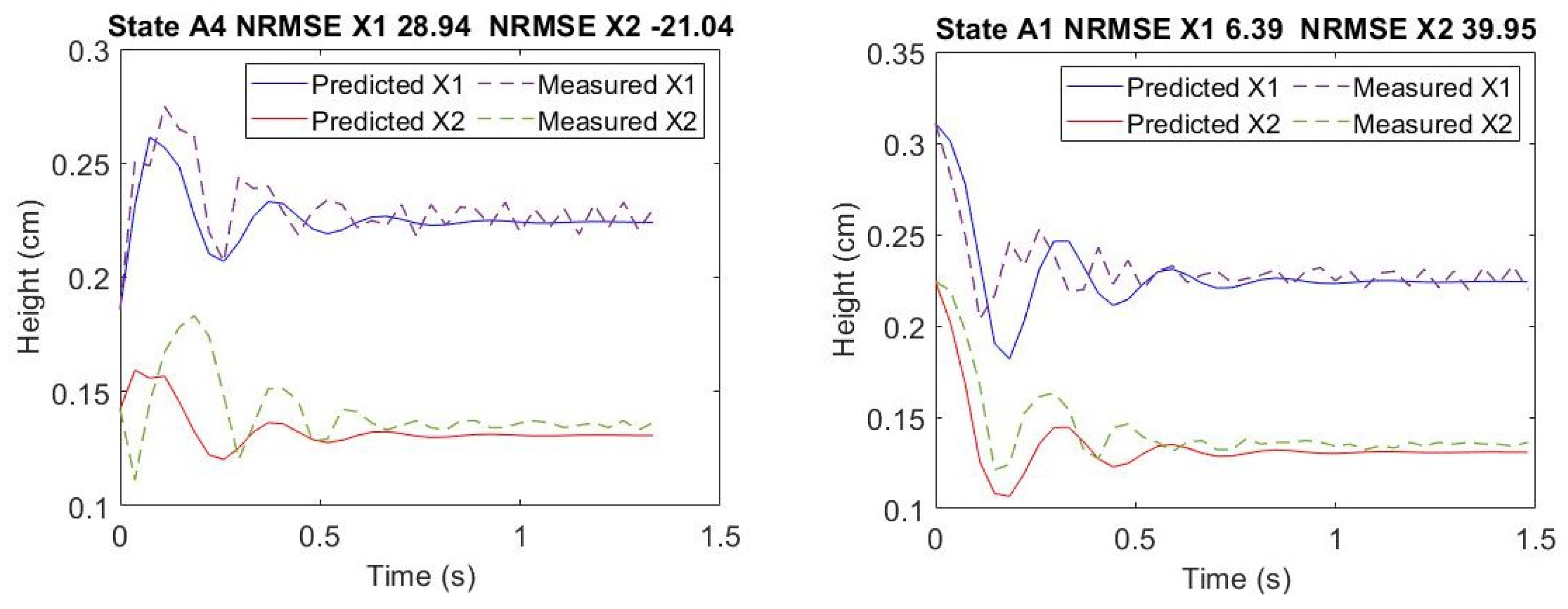
The physical model displays the estimated state and also a proportional number of how close the predicted value output is to the measured data. This number is the Normalized Root Mean Square Error (NRMSE) given in Equation (4) [28], where p is the vector from predict value, m is the vector from measured data, and both have n elements.

$$\begin{array}{c}\hfill NRMSE=\frac{\sqrt{{\sum }_{i=1}^n{(p_i-m_i)}^2}}{\sqrt{{\sum }_{i=1}^n{(p_i-\widehat{p})}^2}}\end{array}$$

(4)

The outlined abnormal situations considered in this case study were devised to meet complex scenarios typically found in landing-gears operation. Abnormal situations addressed in this case study have, at least, one of the following characteristics: high dimensionality, high effort to distinguish boundaries, indirect measurements, and time-variant boundaries.

Table 5. Expected system states.

Label	State	Isolation	Description	Quantity
A1	System Degradation	Spring 1	Spring 1 insufficient stiffness	750
A2	System Degradation	Spring 2	Spring 2 insufficient stiffness	740
A3	Normal		Operation under expected condition	740
A4	Operational Deviation	LNG	High impact due to height	740
A5	Operational Deviation	LNG	High impact due to weight	740

has the expected system states.

Those states were physically simulated in an FDI Workbench, through different release heights, changing springs, and changing weight on the first platform. The physical model can represent any linear or linearized system. Nevertheless, the focus is going to be over a generic three degree of freedom mass-spring-damper model, which is the most suitable for many landing-gear types. There is an assumption that the model parameters are known.

Figure 5 presents the analytical perspective of the experiment. There are three specific physical conditions occurring in different time-space, resulting in a Linear-Parameter-Varying (LPV) approach for this method.

Condition 1 occurs from release moment until, just precisely, before the first impact of $m_3$ over the floor. Free-fall equations rule this behavior. Unlike conditions 2 and 3, the system stabilizes very fast in $L_1$ and $L_2$, that is, oscillations after release are negligible. Condition 2 remains while $m_3$ keeps contact to the floor. Otherwise, the equations in condition 3 describe the physics. It is relevant to notice that condition 3 can replace condition 2 if oscillations have to be considered, but this situation increases the model complexity.

Conditions 2 and 3 have two great differences. One of them is that $k_3$ and $d_3$ are floor stiffness and floor viscous damping coefficients respectively, it is not considered for condition 3, and the second one is that condition 2 has its equilibrium position aligned with specific positions, defined in parameters $p_n$, while condition 3 has its equilibrium through space-intervals defined in $L_1$ and $L_2$ disregarding any specific state-position.

Table 6. Parameters and variables of the Physical Model.

Variables & Symbols	Domain or Space	Description
n	$n\in \mathbb{N}|1\le n\le 3$	Degree of freedom index
$h_0$	$h_n\in \mathbb{R}$	Release height
$k_n$	$k_n\in \mathbb{R}$	Spring stiffness coefficient
$d_n$	$d_n\in \mathbb{R}$	Viscous damping coefficient
$m_n$	$m_n\in \mathbb{R}$	Mass of the body
$S_n$	$S_n\in \mathbb{R}$	Spring force
$D_n$	$D_n\in \mathbb{R}$	Damping force
$W_n$	$W_n\in \mathbb{R}$	Weight force of mass $m_n$
$x_n$	$x_n\in \mathbb{R}$	Actual body position or state-variable
$X(t)$	$X(t)\subset \mathbb{R}$	State vector
$p_n$	$p_n\in \mathbb{R}$	Body position when in static equilibrium on the ground
$L_n$	$L_n\in \mathbb{R}$	Spring length between $m_n$ and $m_{n+1}$ disregarding any external forces effect
$\Delta h_n$	$\Delta h_n\in \mathbb{R}$	Difference between release height and $p_n$
$H_c$	$H_c\subset \mathbb{R},c\in \mathbb{N}|1\le n\le 3$	Observation matrix with respect to condition c
$z_t$	$z_t\in \mathbb{R}$	Measurement vector

details all useful parameters and variables of the method until this moment.

Abnormal situations A1 and A2 are related to wear problems that correspond to equipment degradation. A4 and A5 indicate abnormal situations corresponding to the system operation exceeding the safe operating usage limit.

It is important to highlight that the labels from A1 to A5 correspond to possible states of the target system. From this perspective, abnormal or normal situations are not relevant to the algorithm since the assigned task is just to classify the actual system state in this study case.

However, each state represents a possible normal or abnormal situation that must be monitored in an operational environment. In this way, labels A1 and A2 represent an abnormal situation due to spring degradation, while labels A4 and A5 represent abnormal situations due to operational deviation.

The training, validation and test matrices data-set proportions are 70%, 15%, and 15%, respectively, and they were built in a random process. Despite being a shallow neural network, the Adaptive Moment Estimation (ADAM), generally employed in deep learning techniques, achieved the best results to train the ANN. The accuracy in this step strongly impacts the AM, since the calculations depend on the initial state vector of the system.

The essential purpose behind sets $\Theta$ and $\Gamma$ is to implement different strategies, simultaneously, while the data-sets are divided into smaller random subgroups of data.

Table 7. Selected algorithms.

Set	Inducer	Motivation
$\Theta$	ANN	All input data needs to be in the same range, non-linear, discriminant paradigm, parametric, no distributions assumptions about the model, but data needs to be balanced through different classes.
$\Theta$	LDA	Gaussian distribution and constant variance assumptions for each class, generative paradigm, parametric, it provides dimensionality reduction and linear differentiation between classes.
$\Gamma$	DT	No distributions assumptions, discriminative paradigm, non-parametric, low sensitivity to unbalanced data; however, it becomes unstable when trained with different amounts of data.
$\Gamma$	SVM-RBF	No distributions assumptions, discriminative paradigm, non-parametric, it increases dimensionality to help distinguish data, it depends on the Euclidean distance between two points.

lists the selected algorithms to compose $\Theta$ and $\Gamma$ weak learners.

As seen in Table 7, all of them have some complementary capabilities over each other, and they were built according to the configurations described in

Table 8. ANN configuration.

Phase	Description	Value
Setup
	Number of input features	4 to 8 randomness
	Number of hidden layers (HL)	1
	Number of neurons in HL	5
	HL activation function	Tangent hyperbolic
	Out layer size	5 (equals the number of classes)
	Out layer function	Softmax
Training
	Method	Back-propagation (Gradient descent), ADAM optimizer
	Data distribution	70% training, 15% validation, 15% test
	Stop criterion	Early stop when minimum gradient magnitude
	stabilizes or 25000 epochs
	Learning rate	0.001

,

Table 9. LDA configuration.

Phase	Description	Value
Setup
	Number of input features	5 to 10 randomness
	Covariance matrix	All classes have the same covariance matrix
Training
	Cross-validation	10 k-fold

,

Table 10. DT configuration.

Phase	Description	Value
Setup
	Number of input features	5 to 10 randomness
	Maximum depth	2
	DT algorithm	standard CART
	Optimization criterion	Gini‘s diversity index
Training
	Cross-validation	10 k-fold

and

Table 11. SVM-RBF configuration.

Phase	Description	Value
Setup
	Number of input features	5 to 10 randomness
	Kernel	Radial basis function (RBF)
	Multi-class design	One against all (OVA)
	Optimization	Bayesian optimization
Training
	Cross-validation	10 k-fold

.

LDA does not have hyperparameters to adjust to due to its formulation that works similarly to logistic regression. However, it is possible to choose some variants that make changes in the covariance matrix between classes (e.g., quadratic discriminant analysis QDA).

As observed in configuration tables, a random number of input features, from five to ten, is a common point applied to all algorithms. However, the randomness consists of picking up a feature description vector from a shuffled list. On the other hand, the list was biased to assure that all features were evenly distributed along all vectors.

Before proceeding to the following steps, it is necessary to evaluate if the Ensemble Triads classify better when compared with the situations detailed in

Table 12. Situations to evaluate.

Number	Situation
1	Application of only one kind of algorithm.
2	Gathering all techniques in one ensemble and counting every inducer as one vote.
3	Only parametric sets application.
4	Only non-parametric sets application.
5	All triads heterogeneous sets application.

. They are combinations that represent issues that need to be considered in order to determine if ET implementation is worth it.

4.2. Results

All previous situations can always be analyzed with the same training folds and random distribution seeds since all inducers’ results can be tracked separately. All of them happen at the same time; therefore, it is just a matter of how to combine each one of the results. Consequently, those combination results are shown in Figure A1 and Figure A2 in Appendix A, and must be compared to the results of the whole Ensemble Triads technique showed in Figure A3. The following confusion matrices resume the scenario where Ensemble Triads were ranking better than the other situations from Table 12.

The results were very stable after replicating all of them six times. However, each scenario represented by feature spaces ${\overrightarrow{V}}_a^{26},{\overrightarrow{V}}_b^{14},{\overrightarrow{V}}_c^{12}$ had a different evaluation based on Table 12. The outcomes, when applying feature space ${\overrightarrow{V}}_c^{12}$, are shown from Figure A1, Figure A2 and Figure A3.

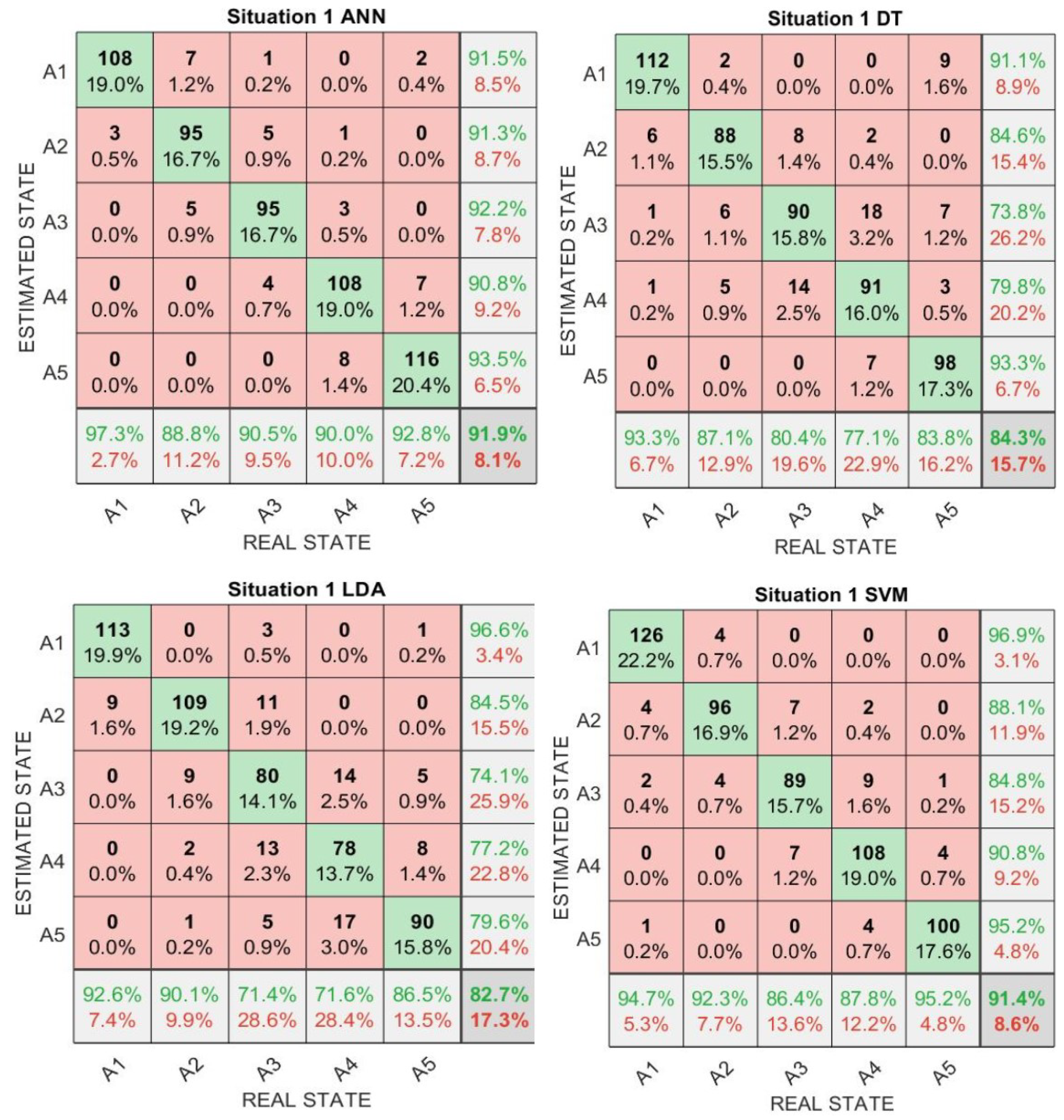
Situation 1 is more sensitive because all algorithms are in a weak and biased format; therefore, it should not be seen as representative of their kinds. However, they represent very well the versions of their Bootstrap Aggregation (Bagging) that consists of ensembles of them.

From the confusion matrices analysis, it is noticed that the accuracy of situation 1 has a high variance among the four selected algorithms, and none of them could perform better than ET. Moreover, it is possible to see that DT and LDA had the worst performances. All inducers are independent in situations 2, 3 and 4, and the difference lies in the fact that situation 2 is a set of all algorithms, while situation 3 is a set composed by ANN-LDA, and situation 4 is composed by DT-SVM. For that reason, since it is a matter of majoritarian vote, situation 2 performed better than the others just because it has twice the number of inducers.

Situation 5 combines all inducers from situation 2 into triads and holds a negligible higher accuracy when they are both compared. However, it indicates that changing the way of combining inducers, instead of leaving them for their own, can increase accuracy. Finally, ET could achieve the best result among all others, mainly because of the same principle that makes situation 2 achieve better results than situations 1, 3 and 4. That is, it aggregates situations 3 and 4, composing their respective triads.

4.2.1. Committee

The feature space ${\overrightarrow{V}}_a^{26}$ was used as input to the comparison between

Table 13. Majority vote decision.

Situation	True Positives						F1 Score
	A1	A2	A3	A4	A5	Total
2	55	55	56	50	44	260	90.98
3	55	52	60	48	42	257	89.75
4	54	54	53	47	37	245	85.68
5	54	55	57	47	43	256	89.47
ET	55	55	57	49	41	257	89.82

and

Table 14. Score balance decision.

Situation	True Positives						F1 Score
	A1	A2	A3	A4	A5	Total
2	55	55	56	50	44	260	90.98
3	55	54	60	45	46	260	90.84
4	54	52	55	46	39	246	86.20
5	55	54	61	45	46	261	91.08
ET	55	55	60	47	46	263	91.90

, and it summarizes the impact of applying score balance algorithm instead of majority voting as the decision-making process used by the committee.

Like many other machine learning techniques, each training pseudo-randomness process is ruled by a seed that yields different combinations for better or worse results and even different ranking positions for those situations. However, all evaluations were performed precisely with the same conditions of seed, training set, training fold, and testing set, which assures a fair analysis.

From the FDI perspective, it was noticed that score balance decisions could easily manage the trade-off between state detection given a specific situation or among the situations. There is a clear understanding when analyzing situation 3 in both tables. Supposing that A4 is much more critical to detect than the others, even a general increase of correct detection may not be desired if A4 has its accurate detection decreased.

After analyzing all results, the answer is that ET is worth because it is proved that in some circumstances, its classification performed better than the others; however, none of the combinations can always guarantee the best results, since it depends on the seed and feature space applied.

Nonetheless, all nine different situations are intrinsic to this technique, and the computational effort necessary to ranking them is negligible if compared to the training one, which makes it possible to declare that there is no reason to disregard any of them. Therefore, given some sorts of algorithms divided into parametric and non-parametric sets, it can assure either the best solution overall among the nine proposed combinations or a better weighted-class solution among situations 3, 4, 5, and ET.

4.2.2. Analytical-Model

The Analytical Model (AM) provides representative levels of the states presented in Table 5. This makes it better to see the cause of abnormal situations A1, A2, A4, and A5, and at the same time, it is possible to follow the degradation levels that occur within the tolerable limits of the system represented by A3.

Table 15. Parameters and variables of the Analytical Model.

Parameter	Value	Description
g	9.806	Considered gravity acceleration in m/s2.
$k_1$	575	Spring 1 stiffness coefficient in N/m.
$k_2$	575	Spring 2 stiffness coefficient in N/m.
$k{d}_1$	405	Simulation spring 1 degradation stiffness coefficient in N/m.
${\widehat{d}}_1$	8	Spring 1 viscous estimated damping coefficient in N.s/m.
${\widehat{d}}_2$	8	Spring 2 viscous estimated damping coefficient in N.s/m.
$m_1$	0.390	Body 1 mass in kg.
$m_2$	0.400	Body 2 mass in kg.
$m_3$	0.340	Body 3 mass in kg.
$L_1$	0.097	Spring 1 length in m.
$L_2$	0.097	Spring 2 length in m.
$L{d}_1$	0.11	Simulation spring 1 degradation length in m.

describes the parameters adjusted for AM where $k{d}_1$ and $L{d}_1$ are the parameters of the spring used to simulate degradation.

The experiment measurements are made in millimeters since the model is based on displacement in this work, and for that, a total of 690 simulations were conducted in a workbench to provide the AM with the first scenario feature space, which has position measurements. The left column in Figure 6 are signals from $k_1$ parametrised spring while the right column is those with $k{d}_1$ parametrised spring. It is possible to notice that the degradation levels simulated by $k_1$ are apparent in that figure and, indeed, it does not happen all the time. Another case in Figure A4 presents two misclassified profiles.

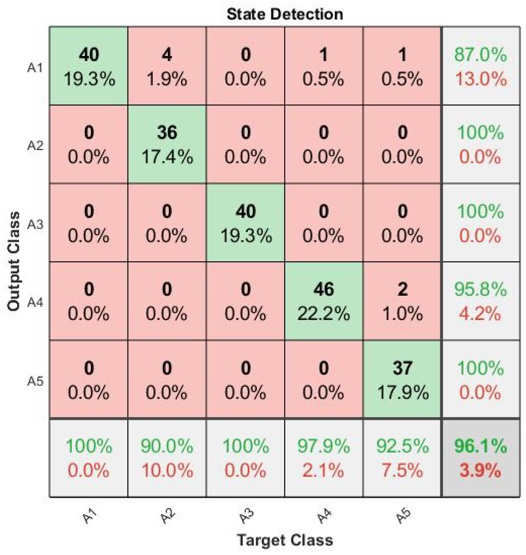
It is necessary to analyze the AM from two perspectives. First, Figure A5 shows the confusion matrix that summarizes state detection accuracy, and the second Figure A6 shows the confusion matrix indicating spring degradation classification regardless of any of the states. This analysis concludes that, alone, the applied AM can achieve accuracy of 96.10% on state detection and accuracy of 93.7% on state isolation in a scenario where displacement measures are provided.

4.2.3. Second Instance-Combining Results

In the previous instance, the results from ET and AM are entirely independent, and now they are gathered in the proposed ANFIS to achieve more accuracy when their results diverge. The 690 simulations based on the first scenario were split into two sets, one with 483 (70%) for training and the other with 207 (30%) for testing, which is from where the results in this subsection came from.

It is remarkable in Figure A7 through both confusion matrices, how the misclassification errors are complementary. The AM performed significantly better in general, even though its false negatives are 10% higher to classify state A2 than the ET technique, which achieved 27.7% of false negatives to classify state A4.

The ANFIS model managed the first results, increasing general accuracy prediction, as seen in Figure A8. It is not possible to describe the process of decision making performed as much as it is challenging to provide a complete set of rules that could explain all expected behavior. However, for the given results, it is possible to state that the proposed ANFIS model has learned those rules adequately.

5. Discussion

As expected, the final instance result provided a better classification capability when compared with the traditional Model-Based approach (Analytical Model) and Data-Driven approach using Ensemble Triads Optimization. As can be observed in Figure A7, the Analytical Model approach was able to perform a correct anomaly classification at 96.1% of the attempts, and the Ensemble Triads Optimization approach was able to classify the anomaly correctly at 91.8% of the attempts. The final instance result, performing the hybridization using ANFIS, achieved a correct classification score of 97.6%, improving model-based or data-driven approaches isolated (see Figure A8).

It is essential to highlight the high dependency of the data-driven approach with the features extraction step. In this work, even considering a model-based approach based on a single model and a comprehensive set of features and using ensemble triads and committees, the model-based approach performed better than the data-driven approach.

It is important to remember that all comparisons were made exactly under the same conditions of seed, training set, training fold, and testing set. This assures a fair analysis of overall results for a single Generic Anomaly Detection Hybridization Algorithm (GADHA) execution. Thus, any change in one of those conditions produces different combinations of prediction algorithms.

All provided machine learning algorithms that need randomness seeds will demand an uncertain number of executions and time to find an appropriate seed that yields better results. This is a common behavior in any situation where this kind of algorithm is employed.

The computational cost depends on the number of selected basic algorithms and their respective performance and abilities, like parallel processing, for example. In this way, this value is the sum of the costs of each of the algorithms independently. However, if the total number of algorithms provided is less than the total number of available processing cores, the processing cost will be equal to the cost of the function with the worst performance.

As the system noise is not modeled, and unpredictable disturbances are usually found in any complex system, data are necessary to differentiate normal behavior signature from abnormal operational conditions or failures response.

The results achieved by the algorithm depend on a balanced number of training data and the desired states to be detected. Like in many data-driven approaches, it is challenging to estimate a minimum amount, but it is possible to find out such value during the experimentation. Considering that there are no algorithms inherent problems, if the minimum desired accuracy for each desired state was not achieved, more training data becomes necessary.

The practical implications of GADHA for scaled industrialization can reduce development time and complexity for a large set of components and subsystems with further impact on development cost.

States A1 and A2 are related to spring degradation, while A4 and A5 are related to operational misuse of the system. Considering the RUL estimation, to better discriminate the states from an abnormal operation of the system to a spring degradation can represent a significant advantage.

Figure 7 will give support to our considerations. The figure may be considered a model-based degradation profile of a given landing-gear system. The Y-axis is the performance of the system and provides the degradation status. The X-axis is the total accumulated stress. P1 and P2 are two different points of degradation and F is the point when the system is in failure condition.

The first detected abnormal condition was the point when an abnormal system state was classified. Many things can be stated. If the point is P1, the predicted RUL is the prediction based on P1 through F and can be expressed in cycles. The same can be declared about P2 and the expected RUL based on P2.

The classification problem can change the perception of the user in terms of the right accumulated stress. If a wrong classification occurs, the predictive-maintenance team could wrongly identify the point and schedule the maintenance in a non-optimal situation.

For example, if the system state is A1 or A2 but was classified as A3 or A4, the team could consider the point P2 as the right one, reducing the expected life of the system. Landing heavier than normal or having a hard landing produce a fast reduction on a landing-gear expected life-time. This situation could generate a financial loss for the user.

If the opposite situation occurs, the hard landing happened but the system identified as a spring stiffness problem, giving the possibility of predicting the system to be in the P1 point. In such a case, late maintenance may occur, and a potential accident could happen if predictive-maintenance dictates the maintenance schedule.

GADHA is designed to be as accurate as possible, bringing the possibility to reuse the framework in many different systems, changing only the parts that are most tied to the target system. The results found so far show that the approach is promising for use in PHM systems.

6. Conclusions

New aircraft generate a large amount of data that allow a series of analyses for both safety and maintenance interests to “more accurately” estimate the condition of various subsystems. In this context, the algorithms identified in this work seek to identify and isolate system states (system degradation, faults, or operational deviation), which can be done through FDI techniques. It does not matter whether the data affect maintenance or safety but whether the necessary parameters are reached to guarantee the operation within tolerable limits of these subsystems.

Several other works addressed solutions for FDI, combining different machine learning techniques or combining one of them with an analytical model, obtaining more accurate results. However, in complex systems cases, the solutions are precise and are generally dedicated to a particular subsystem that responds better to the studied technique. Even in works that require little adaptation, it becomes unfeasible to apply the chosen techniques for that solution, because it is very common for hybrid approaches to be incredibly dependent on its model.

Many of these works then are not used by others due to high degree of forced coupling between the different used algorithms. Despite the primary need to achieve the desired failure detection and isolation rates, it is necessary, whenever possible, to maintain the least degree of coupling possible between algorithms. The reason for this is because it becomes easy to replace the more specific technique of one subsystem for another one without affecting possible dependencies on other parts of the algorithm.

Under the same circumstances, the proposed method demonstrated its ability to combine different techniques in order to achieve equal or better accuracy than its isolated application. It is a matter of fact that since the algorithm can decide which combination or even just one of its techniques yields better results. It is not about a new FDI Method, but a methodology to do hybridization of some provided different techniques analyzed over their isolated and combined ensemble sets’ performance, looking for improved general accuracy. Furthermore, it can combine model-based techniques gathering their decisions on the second instance layer.