Transitional SAX Representation for Knowledge Discovery for Time Series

Abstract

Numerous dimensionality-reducing representations of time series have been proposed in data mining and have proved to be useful, especially in handling a high volume of time series data. Among them, widely used symbolic representations such as symbolic aggregate approximation and piecewise aggregate approximation focus on information of local averages of time series. To compensate for such methods, several attempts were made to include trend information. However, the included trend information is quite simple, leading to great information loss. Such information is hardly extendable, so adjusting the level of simplicity to a higher complexity is difficult. In this paper, we propose a new symbolic representation method called transitional symbolic aggregate approximation that incorporates transitional information into symbolic aggregate approximations. We show that the proposed method, satisfying a lower bound of the Euclidean distance, is able to preserve meaningful information, including dynamic trend transitions in segmented time series, while still reducing dimensionality. We also show that this method is advantageous from theoretical aspects of interpretability, and practical and superior in terms of time-series classification tasks when compared with existing symbolic representation methods.

1. Introduction

Most of the real-world applications, such as financial assessment, weather monitoring, medical data examination, and multimedia systems generate huge amounts of time-series data daily. One of the main characteristics of time series data is high-dimensionality, which leads to the development of efficient data representation techniques that not only reduce the high dimensionality but also preserve the meaningful characteristics. In addition, a desirable distance measure for the reduced time series representation needs to be defined carefully for various data-mining tasks, such as indexing, searching, classification, clustering, motif discovery, anomaly detection, and rule discovery.

Some of the well-known data representations for time series with dimensionality reduction are discrete Fourier transform (DFT) [1], discrete wavelet transform (DWT) [2], discrete cosine transform (DCT) [3], singular value decomposition (SVD) [4], piecewise aggregate approximation (PAA) [5], adaptive piecewise constant approximation (APCA) [6], and symbolic aggregate approximation (SAX) [7]. Most of the above mentioned techniques except for SAX bring forth real-valued representations that are more expensive in terms of storage and computational complexity than symbolic representations for high dimensional time series data. The SAX method transforms real-valued time series data into a symbolic string following two main steps: (1) transforming the original time series to piecewise aggregate approximation (PAA), and (2) converting the PAA represented values into alphabetic symbols based on the assumption that the given normalized data follow normal distribution. Symbolic representations make possible the use of various string-based algorithms, already available, and diverse data structures in time series mining tasks. In addition, the distance measure corresponding to SAX attains a lower bound than popular distance measures defined on the original data. Due to its good performance in storage efficiency, time efficiency, and answer-set correctness (no false dismissals), SAX has been widely used in various applications, such as semantic sensor networks [8], mobile data management [9], and data visualization tools [10].

Though SAX is widely adopted in time series representation for its simplicity and efficiency, it undergoes considerable information loss. The traditional SAX method, however, removes trend and shape information in a time series, assuming that a portion of an arbitrary time series contains intermingled up-and-down trends. SAX basically uses averaged values of subsequences while ignoring trend information. Noticeably, SAX discretization does not guarantee equally probable symbols owing to its intermediate PAA [11]. As PAA is applied before SAX representation, the distribution of the data is altered and results in a shrinking standard deviation. This shrinking distribution negatively affects the symbolic representation of the time series deviating from the target distribution. Recently, researchers have improved SAX representations and the associated distance measures from various aspects to compensate for its information loss. The original SAX representation is integrated with, for example, a modified lookup table and a slope by regression. We explore some improvements related to the SAX representation and the distance measures.

Genetic-algorithm SAX (GASAX) was proposed to determine breakpoints using a genetic algorithm [12]. The objective of GA is to find the nearly optimal configuration of breakpoints that gives the best fitness. The authors argued that the normality assumption oversimplifies the problem of SAX representations and may result in high error when performing time-series mining tasks. Although GASAX works well on both normalized and non-normalized time series data, it needs to define suitable control parameters for its operators and fails to include trend information. Extended SAX (ESAX) [13] enhanced SAX by adding two new points, the maximum and minimum, to the original SAX representation. Using financial time-series data, the research showed that representations of ESAX are more precise than those of SAX without losing the symbolic nature of the original SAX. On the one hand, the storage cost of ESAX is triple that of the original SAX, since it necessarily locates the maximum and minimum along with the sample mean for each segment. Since SAX representations have low accuracy when distinguishing time series with similar average values but different trends, several attempts were made to qualitatively define a few trends, such as slight up/down and substantial up/down. Sun et al. defined a SAX-based trend distance (SAX-TD) quantitatively by using the starting and ending points of a segment and improved the original SAX distance [14].

Yin et al. proposed trend feature symbolic approximation (TFSA) using a two-step segmentation technique for rapid segmentation in long time series data [15]. TFSA, satisfying a lower bound criterion, showed better segmentation and classification accuracy. Malinowski et al. also represented a time series as a sequence of symbols consisting of the average and trend for each segment [16]. Basically, it is an application of linear regression to time series sub-segments, and symbols take into account information on the sample averages and slope values. This method, called 1d-SAX, improved retrieval performance, while the compression ratio remained similar to the original SAX.

In this paper, we propose a new symbolic representation method that incorporates transitional information of values according to time, enabling the method to easily track the direction in which a current symbolic representation moves toward the symbolic aggregate approximation. We aimed to capture important patterns in a systemic and meaningful fashion and append them to a piecewise representation method, such as SAX or PAA, for time series. We chose the SAX method to associate with the proposed method with because of its popularity and performance. Since neither SAX nor PAA suffer from low classification accuracy due to a high level of information compression or information loss, the proposed representation improves classification tasks and preserves interpretability.

The remaining part of this article is organized as follows: Section 2 contains the background of SAX. Section 3 describes the proposed approach for improving SAX with trend information. Section 4 shows experimental designs and results to verify the performance and interpretability of the proposed representation. Section 5 concludes the research with future research directions.

2. Preliminary: PAA and SAX

In this section, we briefly explain preliminary information of SAX. SAX is a time series representation method using piecewise aggregate approximation (PAA) of time-series subsequences. Given a time series $X{\left\{x\left(t\right)\right\}}_{t=1,\dots ,N}$, the PAA divides X into n equally sized segments, $X_p{\left\{x\left(t\right)\right\}}_{t=K(p-1)+1,\dots ,Kp},p=1,\dots ,n$, where N is divisible by $n(n\ll N)$ and $K=N/n$. It evaluates its local average for the p-th segment, $X_p$:

$${\overline{x}}_p=\frac{1}{K}{\sum }_{j=K(p-1)+1}^{Kp}x\left(j\right).$$

(1)

Next, the method transforms X into a representation vector ${\left\{{\overline{x}}_p\right\}}_{p=1,\dots ,n}$, an efficient dimensionality-reduction from N to n, which weakens the noise influence in $x\left(t\right)$. The SAX method maps ${\overline{x}}_p$ into a symbol in consideration of the value space of X. For the mapping, it further divides the value range or value space of segments $X_p$ into several non-uniform regions under the normality assumption and assigns a symbol to each region.

3. The Proposed Method, Transitional SAX

Starting with the definition and transition of value spaces in detail, we introduce the proposed method.

3.1. Transitional Information in Sub Value Spaces

We first assume that the values $x\left(t\right)$ in time series X follow a normal distribution through normalization and detrending, widely adopted in the literature [7,17]. Notice that we choose the original time series X rather than segment $X_p$ to increase the validity of the assumption. We divide the value space into regions with equal probability. To describe the regions in detail, we define a sub value space to be an interval $S_k=[y_{k-1},y_k),k=1,\dots ,\alpha$, such that $\widehat{\Phi }\left(y_k\right)-\widehat{\Phi }\left(y_{k-1}\right)=1/\alpha$, in which $\widehat{\Phi }$ is the cumulative probability function of a normal distribution with the sample average and the sample variance of $x\left(t\right)$. The parameter $\alpha$ is the number of sub value spaces. In the following experiments, we show how to set $\alpha$ through a cross-validation procedure with training datasets. Observe that $y_0$ is the minimum of all values $x\left(t\right)$ and $y_{\alpha }$ is the maximum.

Now given the sub value spaces $S_k$, various feature reduction and extraction approaches are possible for expressing the time series X. For example, the SAX method assigns a symbol for a sub value space, reducing a numerical piecewise approximation to a symbol. In this paper, we aim to include transitional trend information by extracting the transition counts. For segments $X_p$, we count the number of transitions, denoted by ${\gamma }_{i,j}\mathrm{where}i,j=1,\dots ,\alpha$, from sub value space $S_i$ to $S_j$ as follows:

$${\gamma }_{i,j}={\sum }_{t=K(p-1)+1}^{Kp}\mathbf{I}(x\left(t\right)\in S_i)\mathbf{I}(x(t+1)\in S_j),$$

(2)

where $\mathbf{I}\left(A\right)$ is 1 if the relation A is true, and 0 otherwise. Let us define ${\overline{x}}^{\left(i\right)}$ to be the average of $x\left(t\right)$ in sub value space $S_i$: ${\overline{x}}^i=1/\left|S_i\right|{\sum }_{t:x\left(t\right)\in S_i}x\left(t\right).$

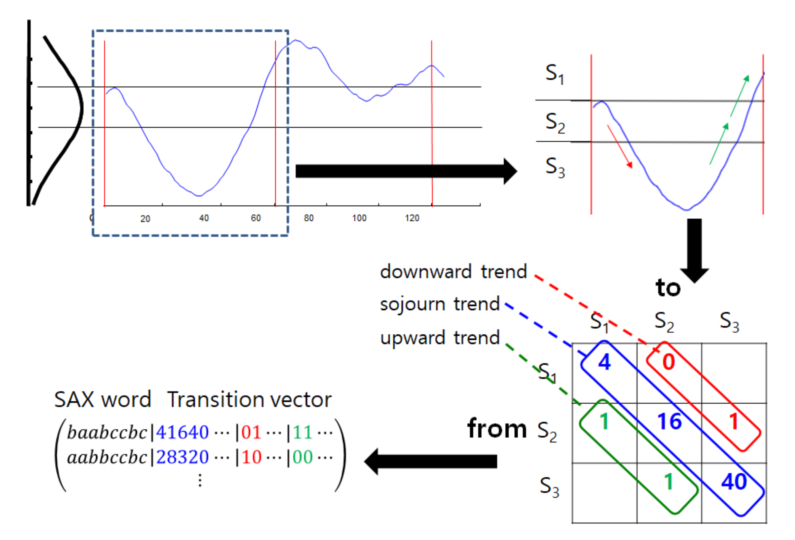
When applying all combinations of sub value spaces, $S_1,S_2,\dots ,S_{\alpha }$, we form a transition matrix, $\gamma =\left[{\gamma }_{i,j}\right]$ of size $\alpha \times \alpha$: element ${\gamma }_{i,j}$ means the number of transitions from $S_i$ to $S_j$. The use of transition matrix $\gamma$ enables us to state terms relating to trend. We call the collection of ${\gamma }_{i,j}$ in which $|i-j|$ is constant a trend. In particular, ${\sum }_{i=1}^{\alpha }{\gamma }_{i,i}$ defines a sojourn trend as the sum of each piece of sojourn information ${\gamma }_{i,i}$. In Figure 1, for instance, $\alpha$ is set to 3, and three sub value spaces, $S_1$, $S_2$, and $S_3$, exist. For the first segment $X_1$, the transitional information of values moving in sub value spaces is stored in $\gamma =\left[\right[4,0,0],[1,16,1],[0,1,40\left]\right]$. While all transitional elements ${\gamma }_{i,j}$ are worthwhile, we focus on one-step upward and downward transitional information with sojourn information. For example, ${\gamma }_{2,1}(=1)$ represents the frequency of one-step upward transitions from the sub value space $S_2$, and ${\gamma }_{2,3}(=1)$ represents that of one-step downward transitions from $S_2$. The diagonal elements, ${\gamma }_{1,1}(=4)$, ${\gamma }_{2,2}(=16)$, and ${\gamma }_{3,3}(=40)$, represent the sojourn trends in the three subspace spaces, respectively. If the sum of one-step upward transitions ${\gamma }_{2,1}+{\gamma }_{3,2}$ is zero, it means non-existence of upward trend and possible downward or steady trend. Observe that $0\le {\gamma }_{i,j}\le n-1$ since the most continuous transition pattern is to remain in a sub value space.

We apply the above-mentioned transitional information to SAX, denoting the proposed approach transitional SAX. The overall algorithm is summarized in Algorithm 1. We notice that, as shown in Algorithm 1, a new representation for time series X of size N is the output in Algorithm 1, $V=[W,Z]$ of size $n(1+{\alpha }^2)$ since each segment produces a symbol for the local average plus ${\alpha }^2$ of the transitional information. Unless N is large enough, meaning a long time series, we recommend the use of one-step upward and downward transitions, $\alpha -1$ counts for each, plus the sojourn transitions instead of all ${\alpha }^2$ counts, which brings the dimensionality of V to $n(3\alpha -1)$. In contrast with SAX which is able to handle incremental data, the proposed transitional SAS is not fully online but segment-wise online, since it is able to append a SAX word and a transition vector of a segment to its representation V. One needs to avoid a quite large n to prevent possible delay for online usage. On the contrary, a quite small n hardly captures transitional movements in the sub value spaces.

As shown in line 12 of Algorithm 1, we use letter symbols ${\alpha }_1=k_1$ and ${\alpha }_2=k_2$ if ${\overline{x}}_{p_1}\in S_{k_1}=[y_{k_1-1},y_{k_1})$ and ${\overline{x}}_{p_2}\in S_{k_2-2}=[y_{k_2-1},y_{k_2})$, respectively, and their distance is given by

$$\begin{array}{c}\hfill dist({\alpha }_1,{\alpha }_2)=max\{y_{max\{k_1,k_2\}-1}-y_{min\{k_1,k_2\}},0\}.\end{array}$$

(3)

The letter distance, if located in either the same value sub space, is zero, and otherwise, it is set by the intermediary value spaces between two sub spaces $S_{k_1}$ and $S_{k_2}$. For example, if ${\overline{x}}_{p_1}\in S_3$ and ${\overline{x}}_{p_2}\in S_3$, i.e., in the same value sub space, the distance becomes zero. For value sub spaces right adjacent to each other, ${\overline{x}}_{p_1}\in S_3$ and ${\overline{x}}_{p_2}\in S_4$, the distance becomes zero since the in-between sub value space does not exist. For ${\overline{x}}_{p_1}\ge {\overline{x}}_{p_2}$, it straightforwardly follows that $k_1\ge k_2$, ${\overline{x}}_{p_1}\ge y_{k_1-1}$, and ${\overline{x}}_{p_2}\le y_{k_2}$, leading to ${\overline{x}}_{p_1}-{\overline{x}}_{p_2}\ge y_{k_1-1}-y_{k_2}=dist({\alpha }_1,{\alpha }_2).$

Algorithm 1 Transitional SAX.

1: Input: time series data $X{\left\{x\left(t\right)\right\}}_{t=1,\dots ,N}$         the length of a segment n,         the number of sub value spaces $\alpha$ 2: Output: transitional symbolic representation V 3: procedure TransitionalSAX($X,n,\alpha$) 4:     Initialize $V\leftarrow \left[\right]$, $W\leftarrow \left[\right]$, $Z\leftarrow \left[\right]$, and set $K=N/n$ 5:     Create sub value spaces $S_k,k=1,\dots ,\alpha$, with equal probability $1/\alpha$ by fitting $x\left(t\right)$ values     to normal distribution 6:     for $p=1,\dots ,K$ do 7:         $X_p{\left\{x\left(t\right)\right\}}_{t=K(p-1)+1,\dots ,Kp}$ 8:         ${\overline{x}}_p=\frac{1}{K}{\sum }_{j=K(p-1)+1}^{Kp}x\left(j\right)$ 9:     end for 10:     Set $\rho ={min}_{p,p^{\prime }=1,\dots ,K}\left\{\right|{\overline{x}}_p-{\overline{x}}_{p^{\prime }}\left|\right\}$ 11:     for each segment $X_p,p=1,\dots ,K$ do 12:         Compute local average ${\overline{x}}_p$ and assign a symbol ${\alpha }_k(=w)$ if ${\overline{x}}_p\in S_k$ 13:         $W\leftarrow [W,w]$ 14:         for each $i,j=1,\dots ,\alpha$ do 15:            Compute transitional information                ${\gamma }_{i,j}={\sum }_{t=K(p-1)+1}^{Kp}\mathbf{I}(x\left(t\right)\in S_i)\mathbf{I}(x(t+1)\in S_j)$ 16:            Update Z                $Z\leftarrow [Z,{\gamma }_{i,j}]$ 17:         end for 18:     end for 19:     Update $V\leftarrow [W,Z]$     return V 20: end procedure

3.2. Distance Measure for Transitional SAX

We evaluate the proposed method by how closely the new representation $V=[W,Z]$ of a time series, X, approximates the original time series X. The new distance measure associated with the new representation needs to satisfy a lower-bounding property to ensure no false dismissals [17,18]. For that purpose, we propose the following distance measure. Let us suppose that the transitional SAX method produces new representations $V^{\left(1\right)}=[W^{\left(1\right)},Z^{\left(1\right)}]$ and $V^{\left(2\right)}=[W^{\left(2\right)},Z^{\left(2\right)}]$ for $X_1$ and $X_2$, respectively, with the same size, in which $\tau$ is the size of $Z^{\left(1\right)}$ or $Z^{\left(2\right)}$, $\tau =|Z^{\left(1\right)}|=|Z^{\left(2\right)}|$; we define $D(·,·)$ to be:

$$D(V_1,V_2)=\sqrt{{\sum }_{i=1}^{n}K{(W^{\left(1\right)}\left(i\right)-W^{\left(2\right)}\left(i\right))}^2·{\sum }_{j=1}^{\tau }\frac{{(Z^{\left(1\right)}\left(j\right)-Z^{\left(2\right)}\left(j\right))}^2}{\tau {(n-1)}^2}}.$$

(4)

We compare the distance measure (4) with the Euclidean distance of the original time series to verify that it satisfies the lower-bound condition: we show that $D(V_1,V_2)\le D_{Euclidean}(X_1,X_2)$. The right-hand side of the inequality becomes:

$$\begin{array}{c}\hfill \begin{array}{cc}\hfill & D_{Euclidean}^2(X_1,X_2)={\sum }_{t=1}^N{(x_1\left(t\right)-x_2\left(t\right))}^2={\sum }_{p=1}^n{\sum }_{t=K(p-1)+1}^{Kp}{(x_1-x_2)}^2\hfill \\ \hfill & ={\sum }_{p=1}^n{\sum }_{t=K(p-1)+1}^{Kp}{(x_1\left(t\right)-{\overline{x}}_{1,p}+{\overline{x}}_{1,p}-x_2\left(t\right)+{\overline{x}}_{2,p}-{\overline{x}}_{2,p})}^2.\hfill \end{array}\end{array}$$

(5)

Since the sum of values centered by the average is zero, that is to say,

$$\begin{array}{c}\hfill \begin{array}{cc}\hfill & {\sum }_{p=1}^n{\sum }_{t=K(p-1)+1}^{Kp}(x_1\left(t\right)-{\overline{x}}_{1,p}-x_2\left(t\right)+{\overline{x}}_{2,p})\hfill \\ \hfill & ={\sum }_{p=1}^n{\sum }_{t=K(p-1)+1}^{Kp}(x_1\left(t\right)-{\overline{x}}_{1,p})-{\sum }_{p=1}^n{\sum }_{t=K(p-1)+1}^{Kp}(x_2\left(t\right)-{\overline{x}}_{2,p})=0,\hfill \end{array}\end{array}$$

the right-hand side of Equation (5) becomes

$$\begin{array}{c}\hfill \begin{array}{cc}\hfill & {\sum }_{p=1}^n{\sum }_{t=K(p-1)+1}^{Kp}{(x_1\left(t\right)-{\overline{x}}_{1,p}-x_2\left(t\right)+{\overline{x}}_{2,p})}^2+{\sum }_{p=1}^n{\sum }_{t=K(p-1)+1}^{Kp}{({\overline{x}}_{1,p}-{\overline{x}}_{2,p})}^2\hfill \\ \hfill & \ge {\sum }_{p=1}^n{\sum }_{t=K(p-1)+1}^{Kp}{({\overline{x}}_{1,p}-{\overline{x}}_{2,p})}^2\ge {\sum }_{p=1}^n{\sum }_{t=K(p-1)+1}^{Kp}{(W^{\left(1\right)}\left(p\right)-W^{\left(p\right)}\left(i\right))}^2\hfill \end{array}\end{array}$$

(6)

The last inequality ${({\overline{x}}_{1,p}-{\overline{x}}_{2,p})}^2\ge {(W^{\left(1\right)}\left(p\right)-W^{\left(2\right)}\left(p\right))}^2$ holds true by the letter-distance definition given in Equation (3). The value $Z\left(j\right)$ difference is lower bounded by ${|Z}^{\left(1\right)}\left(j\right){-Z}^{\left(2\right)}\left(j\right)|\le max\left\{Z^{\left(1\right)}\left(j\right)\right\}-min\left\{Z^{\left(2\right)}\left(j\right)\right\}=n-1$, ${\left(Z^{\left(1\right)}\left(j\right){-Z}^{\left(2\right)}\left(j\right)\right)}^2/{(n-1)}^2\le 1$, and

$$\begin{array}{c}\hfill 1\ge {\sum }_{j=1}^{\tau }\frac{{{(Z}^{\left(1\right)}\left(j\right){-Z}^{\left(2\right)}\left(j\right))}^2}{\tau {(n-1)}^2}.\end{array}$$

(7)

The combination of the right-hand sides of equations and (6) and (7) produces

$${\sum }_{p=1}^n{\sum }_{t=K(p-1)+1}^{Kp}{(W^{\left(1\right)}\left(i\right)-W^{\left(2\right)}\left(i\right))}^2\ge {\sum }_{p=1}^{n}K{(W^{\left(1\right)}\left(i\right)-W^{\left(2\right)}\left(i\right))}^2·{\sum }_{j=1}^{\tau }\frac{{{(Z}^{\left(1\right)}\left(j\right){-Z}^{\left(2\right)}\left(j\right))}^2}{\tau {(n-1)}^2},$$

finalizing the proof of $D(V_1,V_2)\le D_{Euclidean}(X_1,X_2)$. By admitting that tight lower-bounds bring forth better contractive property, the lower-bound relation of the associated distance measure implies the utility of the proposed transitional information in distance computation. We will elaborate on its attributes in more detail in the Experiments section.

4. Experiments

4.1. Dataset

We used twenty UCR time series benchmarking datasets [19] to compare the proposed method with the previous algorithms.

Table 1. The description of twenty UCR datasets.

No.	Name	# of Classes	Size of Training Set	Size of Test Set	Length of Time Series
1	Synthetic_control	6	300	300	60
2	GunPoint	2	50	150	150
3	CBF	3	30	900	128
4	FaceAll	14	560	1690	131
5	OSULeaf	6	200	242	427
6	SwedishLeaf	15	500	625	128
7	50Words	50	450	455	270
8	Trace	4	100	100	275
9	TwoPatterns	4	1000	4000	128
10	Wafer	2	1000	6164	152
11	FaceFour	4	24	88	350
12	Lighting2	2	60	61	637
13	Lighting7	7	70	73	319
14	ECG	2	100	100	96
15	Adiac	37	390	391	176
16	Yoga	2	300	3000	426
17	Fish	7	175	175	463
18	Beef	5	30	30	470
19	Coffee	2	28	28	286
20	OliveOil	4	30	30	570

describes the characteristics of the datasets, such as the number of classes, the size, and so forth. We split each dataset into training and testing sets as described in the table. The number of classes varied from 2 to 50. Training and testing set sizes were various from two dozen to thousands. The length of the time series ranged from 60 to 637.

4.2. Methods in Comparison and Parameter Settings

We compared the classification accuracy of our proposed method on one of the major time series data mining tasks symbolic, aggregate approximation, with the transition matrix (denoted as SAX-TM), the classic Euclidean distance (ED), SAX [10], SAX-TD [14], and SAX-SD [18]. We chose classification by one nearest neighbor (1NN) as the performance criterion, following most studies in time series representation [7,10,14]. The advantage of 1NN in time series representation is that the underlying distance measure is critical to the performance of the 1NN classifier. Therefore, the error rate of the 1NN classifier directly reflects the effectiveness of distance measures. Besides, the 1NN classifier is directly comparable with diverse distance measures, since it is parameter-free.

To obtain the best accuracy for each method, we used all training data to search for the best parameters n and $\alpha$. For a given time series of length N, we chose the two parameters n and $\alpha$ using the following criteria. To make the comparison fair, the criteria were the same as those in [17]: for n, we searched from 2 up to $N/2$, doubling the value each time; for $\alpha$, we searched from 3 up to 10. If two sets of parameter settings produced the same classification error rate, we chose the smaller set. We mention that, given labeled data, a training phase will boost not only SAX-TM but also other SAX methods; the traditional SAX needs to set the number of letters among other parameters. With the absence of labeled data, one needs to set the parameters for the SAX methods, including SAX-TM, according to other criteria in an unsupervised manner.

4.3. Experimental Results

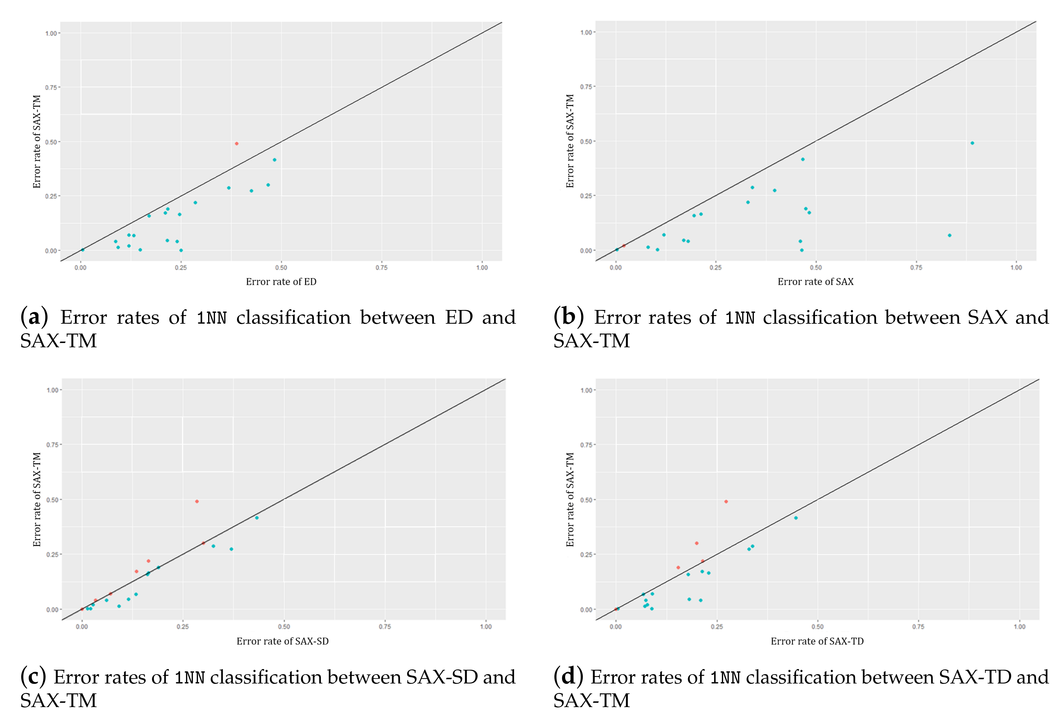
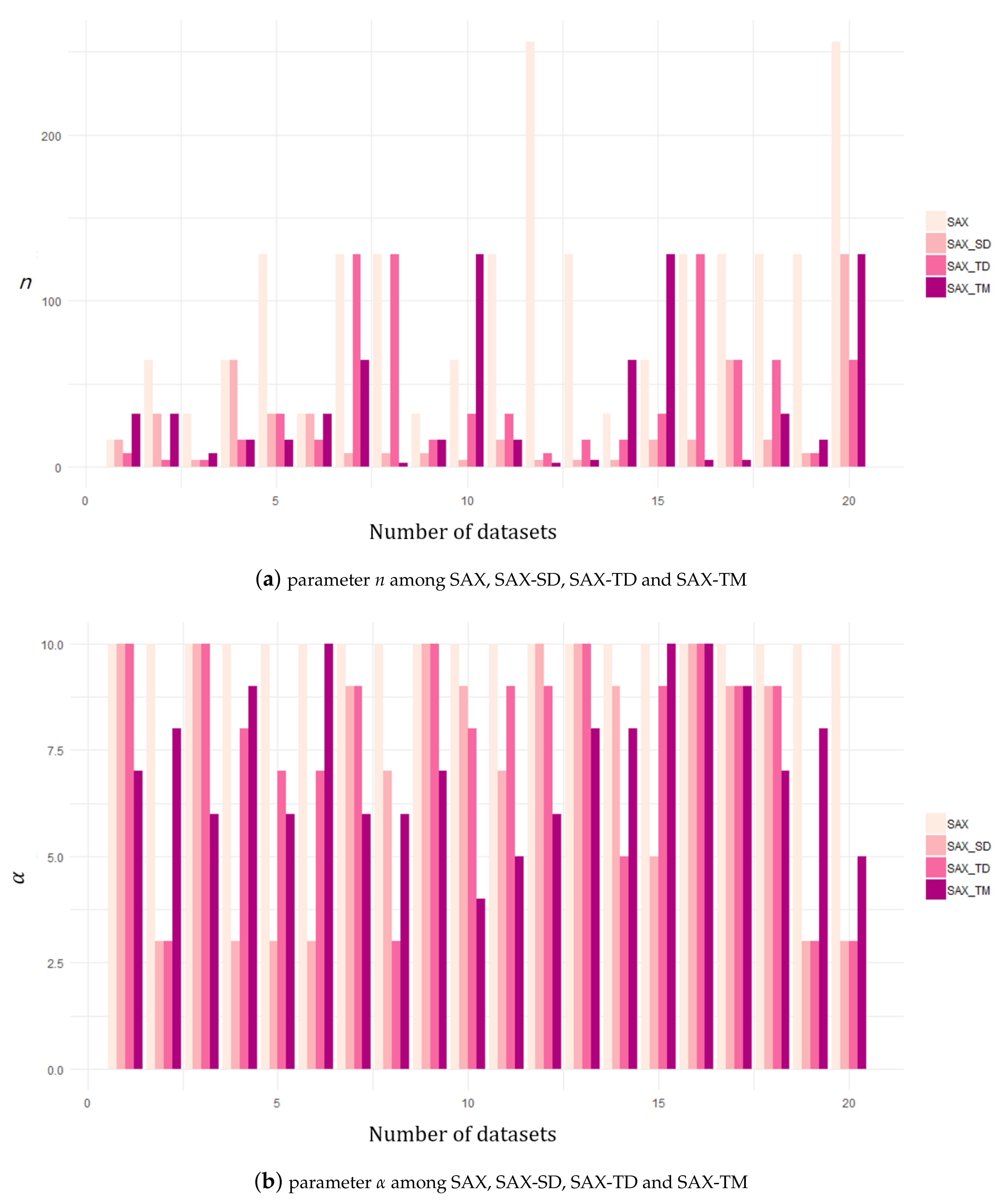
The overall classification results for the testing datasets are listed in

Table 2. 1NN classification error rates of ED (Euclidean distance); 1NN best classification error rates, length n, and dimensionality reduction ratio $\alpha$ of the SAX, SAX-TD, SAX-SD, and SAX-TM on 20 datasets. The lowest error rates are highlighted in bold.

No.	ED Error	SAX Error	SAX n	SAX $\mathit{\alpha }$	SAX -TD Error	SAX -TD n	SAX -TD $\mathit{\alpha }$	SAX -SD Error	SAX -SD n	SAX -SD $\mathit{\alpha }$	SAX -TM Error	SAX -TM n	SAX -TM $\mathit{\alpha }$
1	0.120	0.020	16	10	0.077	8	10	0.027	16	10	$\mathbf{0.020}$	32	7
2	0.087	0.180	64	10	0.073	4	3	$\mathbf{0.033}$	32	3	0.04	32	8
3	0.148	0.104	32	10	0.088	4	10	0.020	4	10	$\mathbf{0.001}$	8	6
4	0.286	0.330	64	10	0.215	16	8	$\mathbf{0.164}$	64	3	0.219	16	9
5	0.483	0.467	128	10	0.446	32	7	0.433	32	3	$\mathbf{0.417}$	16	6
6	0.211	0.483	32	10	0.213	16	7	$\mathbf{0.134}$	32	3	0.171	32	10
7	0.369	0.341	128	10	0.338	128	9	0.325	8	9	$\mathbf{0.286}$	64	6
8	0.240	0.460	128	10	0.21	128	3	0.060	8	7	$\mathbf{0.040}$	2	6
9	0.093	0.081	32	10	0.071	16	10	0.091	8	10	$\mathbf{0.013}$	16	7
10	0.005	0.003	64	10	0.004	32	8	0.013	4	9	$\mathbf{0.003}$	128	4
11	0.216	0.17	128	10	0.181	32	9	0.114	16	7	$\mathbf{0.045}$	16	5
12	0.246	0.213	256	10	0.229	8	9	$\mathbf{0.164}$	4	10	$\mathbf{0.164}$	2	6
13	0.425	0.397	128	10	0.329	16	10	0.370	4	10	$\mathbf{0.274}$	4	8
14	0.120	0.120	32	10	0.090	16	5	$\mathbf{0.070}$	4	9	$\mathbf{0.070}$	64	8
15	0.389	0.890	64	10	$\mathbf{0.273}$	32	9	0.284	16	5	0.491	128	10
16	0.17	0.195	128	10	0.179	128	10	0.162	16	10	$\mathbf{0.158}$	4	10
17	0.217	0.474	128	10	$\mathbf{0.154}$	64	9	0.189	64	9	0.189	4	9
18	0.467	0.567	128	10	$\mathbf{0.200}$	64	9	0.3	16	9	0.3	32	7
19	0.25	0.464	128	10	$\mathbf{0.000}$	8	3	$\mathbf{0.000}$	8	3	$\mathbf{0.000}$	16	8
20	0.133	0.833	256	10	$\mathbf{0.067}$	64	3	0.133	128	3	$\mathbf{0.0670}$	128	5
average	0.234	0.340			0.172			0.154			$\mathbf{0.148}$

, where the lowest classification error is highlighted. Clearly, SAX-TM has the lowest error in most of the datasets ($14/20$), followed by the SAX-SD ($6/20$). On average, the classification error for SAX-TM is lower than half of that for the original SAX in 19 datasets among the 20 datasets. The number of sub value spaces, i.e., the dimensionality reduction ratio, $\alpha$, for SAX-TM is smaller than those for the others except SAX-SD. Figure 2 shows comparisons of SAX-TM with ED, SAX, SAX-TD, and SAX-SD, respectively, in terms of error rates of 1NN classification. Figure 3a depicts changes of n parameters among SAX, SAX-SD, SAX-TD, and SAX-TM, and Figure 3b illustrates changes of parameter $\alpha$ among the comparative algorithms. In addition to the classification performance, we present the computation time of the proposed method in comparison with the original SAX. The comparison bears significance that SAX-TM requires a memory of size $n(1+{\alpha }^2)$ for symbols, whereas the original SAX requires that of size n, as mentioned in Section 3.1. For this comparison, we used three datasets (Lighting2, SpaceShuttle, ECG2) of lengths 637, 5000, and $21,600$; see the results in

Table 3. Comparison of computation time in seconds between SAX and SAX-TM for the three datasets (Lighting2, SpaceShuttle, ECG2) of length 637, 5000, and 21,600, respectively.

	Lighting2		SpaceShuttle		ECG2
$\mathit{n}$	SAX	SAX-TM	SAX	SAX-TM	SAX	SAX-TM
16	0.00071	0.00757	0.00169	0.06058	0.00143	0.2883
32	0.00047	0.00722	0.00128	0.05236	0.00060	0.2563
64	0.00057	0.01095	0.00260	0.05413	0.01102	0.2491
128	0.00129	0.01344	0.00419	0.05911	0.03463	0.2185
256	0.00342	0.01793	0.01397	0.05850	0.08983	0.2199
avg.	0.00129	0.01142	0.00475	0.05693	0.02750	0.2464
std.	0.00110	0.00397	0.00472	0.00314	0.03349	0.0258

. The environment for the comparison was Matlab R2020b and Intel(R) Xeon(R) Platinum 8259CL CPU @ 2.50GHz with $\alpha =10$. We observed that SAX is quite a lot faster than SAX-TM, which is reasonable since SAX-TM requires additional point-wise testing and storage for sub value spaces. The computation times for both methods, increasing according to the dataset length, are reasonably fast. Noticeably, the speed of SAX-TM is relatively robust against n; SAX becomes quite much slow when n changes from 128 to 256 and SAX-TM hardly changes in speed; the standard deviation of SAX-TM is smaller than that of SAX in SpaceShuttle and ECG2.

4.4. Information Analysis

Next, we evaluate the performance of SAX-TM from the viewpoint of information. SAX has been regarded as a de facto standard to reduce the dimensionality of time series data. Despite its popularity and universality, the structural properties of SAX from the information viewpoint have been rarely researched to the best of our knowledge.

Among the statistical facets, Song et al. proposed in the investigation of time-series dimensionality reduction [20] that we focus on information loss and efficiency of information embedding. Both minimizing the loss of useful information and preserving useful information in a raw time series are practical goals. Thus, we adopted procedures to discover intrinsic properties of the proposed method from the perspective of information loss and information embedding.

For this purpose, we calculated the information loss, denoted by $L_{info}$, by mean squared error (MSE) between a raw signal and reconstructed symbolic words:

$$L_{info}(\tilde{T},T)=\frac{\sum {({\tilde{t}}_i-t_i)}^2}{n-1},{\tilde{t}}_i\in \tilde{T},t_i\in T,$$

(8)

in which T is raw signal and $\tilde{T}$ is a reconstructed one. To conduct the comparison, we scaled raw time series and SAX words to $[0,1]$. We also calculated the Kullback–Leibler (KL) divergence, which is a non-symmetric similarity measure between two different probability distributions. For distributions P and Q with k points, the KL divergence is defined as follows:    

$$KL(P\Vert Q)={\sum }_{i=1}^k{p}_{i}log\frac{p_i}{q_i},p_i\in P,q_i\in Q$$

(9)

In our experiments, we take P as the distribution of the original signal T and Q as that of the reconstructed signal $\tilde{T}$ by a histogram with $\alpha$ as the number of bins.

Information loss measures the amount of information abandoned when converting the original time series to a symbolic representation. KL-divergence represents the closeness between the distribution of a raw signal and that of a reconstructed signal. To combine the two measures, Song et al. defined information embedding cost (IEC) as a ratio of KL-divergence and information loss as follows:

$$IE{C}_T(P,Q)=\frac{K{L}_T(P\Vert Q)}{1+L_{info}(\tilde{T},T)}.$$

(10)

Given a time series T in distribution P and reconstructed signal $\tilde{T}$ with distribution Q, the IEC score describes the number of extra bits needed to transform the output $\tilde{T}$ when information loss incurs by one unit, revealing how much useful information is abandoned when transforming a raw signal [20]. A higher value of information loss and a lower value of KL-divergence imply that the reconstruction preserves a large quantity of information while reducing complexity. Hence, we prefer a representation method with lower IEC.

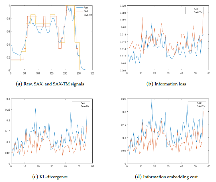
For intuitive understanding, we graphically compare SAX with the proposed method using one representative coffee dataset, providing only performance summaries for the others. Figure 4a shows the raw time series together with representations by SAX and SAX-TM for the coffee dataset. SAX and SAX-TM affordably follow up the shape of the raw signal. In Figure 4b, the information loss of SAX-TM is higher than that of SAX. This means SAX-TM lost much more information than SAX. However, the KL-divergence value of SAX-TM is lower than that of SAX, as shown in Figure 4c. The tendency is also preserved in the IEC scores shown in Figure 4d.

We used twelve datasets in total, including the coffee one, to see the amount of useful information preserved in terms of the information loss, KL-divergence, IEC score, and 1NN classification error. The comparative results between SAX and the proposed method are shown in

Table 4. Information loss and efficiency of information embedding in SAX and SAX-TM.

Dataset	N	Information Loss		KL-Divergence		IEC Score		Classification Error
		SAX	SAX-TM	SAX	SAX-TM	SAX	SAX-TM	Raw Data	SAX	SAX-TM
50words	270	0.056	0.06	0.323	0.355	0.304	0.332	0.361	0.338	0.286
Adiac	176	0.009	0.189	0.07	0.103	0.07	0.087	0.407	0.383	0.491
Beef	470	0.038	0.03	0.346	0.493	0.332	0.477	0.4	0.466	0.3
Coffee	286	0.014	0.016	0.123	0.088	0.122	0.086	0.25	0.107	0
ECG	96	0.053	0.084	0.504	0.44	0.474	0.405	0.11	0.22	0.07
Face(four)	350	0.069	0.104	0.597	0.702	0.556	0.631	0.276	0.171	0.158
Gun-point	150	0.025	0.027	0.357	0.35	0.346	0.338	0.13	0.17	0.04
Lighting2	637	0.112	0.387	0.969	0.934	0.862	0.666	0.197	0.229	0.164
Lighting7	319	0.123	0.232	0.912	0.898	0.8	0.716	0.37	0.397	0.274
Oliveoil	570	0.064	0.121	0.261	0.342	0.246	0.305	0.233	0.166	0.067
SwedishLeaf	128	0.025	0.015	0.174	0.142	0.169	0.14	0.201	0.441	0.171
Synthetic control	60	0.092	0.073	0.2	0.158	0.182	0.148	0.12	0.02	0.02
Average		0.057	0.112	0.403	0.417	0.372	0.361	0.255	0.259	0.17

, where N is the data length. We applied the same parameter settings for SAX as in [20] and applied the combination of parameters from Table 2 for SAX-TM.

Overall, in Table 4, information loss of SAX is lower than that of SAX-TM. That is, SAX loses smaller quantities of information than SAX-TM. However, the KL-divergence values of SAX-TM are mostly lower than those of SAX: the number of lower KL-divergence for SAX-TM ($7/12$) is larger than that for SAX ($5/12$). This tendency is preserved in the IEC score. Even the average IEC scores for SAX-TM are lower than those for SAX. That is, SAX-TM loses less useful information than SAX. Nevertheless, the 1NN classification error of SAX-TM is considerably lower than that of SAX. By appending transitional information to the original SAX, we obtained substantial gains in accuracy.

5. Conclusions

In this work, we described the popularity and universality of SAX, which is a symbolic aggregate approximation in the field of dimensionality reduction for time series data. The original SAX barely captures trend information from the perspective of time-series shape. Therefore, we proposed a symbolic aggregate approximation with transitional information, which can represent trend information by appending transition information to basic SAX.

In a given time window, a SAX word is created, and we can trace how data points travel from the current quantile region to the next location. We call this moving behavior from the current location to the next location a transition. When in a current location, data points in a window can choose from three movements—upward transition, downward transition, and sojourn transition. These movements are saved in the data format of a matrix. First, we conducted experiments to verify the effectiveness of SAX-TM compared with other state-of-the-art methods such as SAX-TD and SAX-SD. The experimental results show SAX-TM has the lowest 1NN classification error among the algorithms. Next, we identified intrinsic statistical properties of SAX-TM. From [20], we selected information loss, KL-divergence, and information embedding cost as important measurements. Overall, the information loss of SAX is lower than that of SAX-TM. However, the number of datasets with lower KL-divergence for SAX-TM is slightly larger than that for SAX. This tendency is also preserved in terms of the IEC score. Nonetheless, SAX-TM substantially reduces classification error compared with SAX. SAX-TM shows explicit increases in accuracy even while appending transition information to SAX.

In spite of the aforementioned advantages, the proposed algorithm has several limitations. Basically, SAX compresses raw data for smoothing. However, SAX-TM increases the complexity of SAX representation by appending a transition matrix. We plan to investigate the minimal effective information to add to SAX and compare it with well-known non-SAX methods. In addition, future research directions include the theoretical aspects of the transition information in several time-series models.

References

- Agrawal, R.; Faloutsos, C.; Swami, A.N. Efficient similarity search in sequence databases. In Proceedings of the 4th International Conference on Foundations of Data Organization and Algorithms FODO’93, 1993, Chicago, IL, USA, 13–15 October 1993; Springer: Berlin/Heidelberg, Germany, 1993; pp. 69–84. [Google Scholar]
- Chan, K.P.; Fu, A.W.-C. Efficient time series matching by wavelets. In Proceedings of the 15th International Conference on Data Engineering (Cat. No.99CB36337), Sydney, Australia, 23–26 March 1999; pp. 126–133. [Google Scholar]
- Korn, F.; Jagadish, H.V.; Faloutsos, C. Efficiently supporting ad hoc queries in large datasets of time sequences. SIGMOD Rec. 1997, 26, 289–300. [Google Scholar] [CrossRef]
- Kanth, K.V.R.; Agrawal, D.; Singh, A. Dimensionality reduction for similarity searching in dynamic databases. In Proceedings of the 1998 ACM SIGMOD International Conference on Management of Data, SIGMOD’98, Seattle, WA, USA, 2–4 June 1998; ACM: New York, NY, USA, 1998; pp. 166–176. [Google Scholar]
- Keogh, E.J.; Chakrabarti, K.; Pazzani, M.J.; Mehrotra, S. Dimensionality reduction for fast similarity search in large time series databases. Knowl. Inf. Syst. 2001, 3, 263–286. [Google Scholar] [CrossRef]
- Chakrabarti, K.; Keogh, E.; Mehrotra, S.; Pazzani, M. Locally adaptive dimensionality reduction for indexing large time series databases. ACM Trans. Database Syst. 2002, 27, 188–228. [Google Scholar] [CrossRef]
- Lin, J.; Keogh, E.; Lonardi, S.; Chiu, B. A symbolic representation of time series, with implications for streaming algorithms. In Proceedings of the 8th ACM SIGMOD Workshop on Research Issues in Data Mining and Knowledge Discovery, DMKD ’03, San Diego, CA, USA, 13 June 2003; ACM: New York, NY, USA, 2003; pp. 2–11. [Google Scholar]
- Barnaghi, P.M.; Ganz, F.; Henson, C.A.; Sheth, A.P. Computing perception from sensor data. In Proceedings of the 2012 IEEE Sensors, Taipei, Taiwan, 17 January 2013; pp. 1–4. [Google Scholar]
- Tayebi, H.; Krishnaswamy, S.; Waluyo, A.B.; Sinha, A.; Gaber, M.M. Ra-sax: Resource-aware symbolic aggregate approximation for mobile ecg analysis. In Proceedings of the 2011 IEEE 12th International Conference on Mobile Data Management, Lulea, Sweden, 6–9 June 2011; Volume 1, pp. 289–290. [Google Scholar]
- Li, H.; Yang, L. Time series visualization based on shape features. Knowl.-Based Syst. 2013, 41, 43–53. [Google Scholar] [CrossRef]
- Butler, M.; Kazakov, D. Sax discretization does not guarantee equiprobable symbols. IEEE Trans. Knowl. Data Eng. 2015, 27, 1162–1166. [Google Scholar] [CrossRef]
- Fuad, M.M.M. Genetic algorithms-based symbolic aggregate approximation. In Proceedings of the 14th International Conference on Data Warehousing and Knowledge Discovery, Vienna, Austria, 3–6 September 2012; Springer: Berlin/Heidelberg, Germany, 2012; pp. 105–116. [Google Scholar]
- Lkhagva, B.; Suzuki, Y.; Kawagoe, K. New time series data representation esax for financial applications. In Proceedings of the 22nd International Conference on Data Engineering Workshops (ICDEW’06), Atlanta, GA, USA, 3–7 April 2006; p. x115. [Google Scholar]
- Sun, Y.; Li, J.; Liu, J.; Sun, B.; Chow, C. An improvement of symbolic aggregate approximation distance measure for time series. Neurocomputing 2014, 138, 189–198. [Google Scholar] [CrossRef]
- Yin, H.; Yang, S.; Zhu, X.; Ma, S.-B.; Zhang, L. Symbolic representation based on trend features for knowledge discovery in long time series. Front. Inf. Technol. Electron. Eng. 2015, 16, 744–758. [Google Scholar] [CrossRef]
- Malinowski, S.; Guyet, T.; Quiniou, R.; Tavenard, R. 1d-sax: A novel symbolic representation for time series. In Proceedings of the 12th International Symposium on Advances in Intelligent Data Analysis XII—Volume 8207, London, UK, 17–19 October 2013; Springer: Berlin/Heidelberg, Germany, 2013; pp. 273–284. [Google Scholar]
- Lin, J.; Keogh, E.J.; Wei, L.; Lonardi, S. Experiencing sax: A novel symbolic representation of time series. Data Min. Knowl. Discov. 2007, 15, 107–144. [Google Scholar] [CrossRef] [Green Version]
- Zan, C.T.; Yamana, H. An improved symbolic aggregate approximation distance measure based on its statistical features. In Proceedings of the 18th International Conference on Information Integration and Web-based Applications and Services, Singapore, 28–30 November 2016; ACM: New York, NY, USA, 2016; pp. 72–80. [Google Scholar]
- Chen, Y.; Keogh, E.; Hu, B.; Begum, N.; Bagnall, A.; Mueen, A.; Batista, G. The Ucr Time Series Classification Archive. July 2015. Available online: www.cs.ucr.edu/~eamonn/time_series_data/ (accessed on 5 October 2020).
- Song, W.; Wang, Z.; Zhang, F.; Ye, Y.; Fan, M. Empirical study of symbolic aggregate approximation for time series classification. Intell. Data Anal. 2017, 21, 135–150. [Google Scholar] [CrossRef]
Figure 1.
Graphical description of transitional SAX.
Figure 2.
Comparison of error rates in 1NN classification between the existing methods and the proposed algorithm.
Figure 3.
Parameters among SAX, SAX-SD, SAX-TD, and SAX-TM.
Figure 4.
Performance comparison of SAX and the proposed method on the coffee dataset.