Performance Degradation Analysis and Optimization of the Stepless Capacity Regulation System for Reciprocating Compressors

Abstract

The regulating performance degradation of the stepless capacity regulation system for reciprocating compressors occurs frequently in long-term operations. It affects the safe and stable operation of the compressor seriously. The degradation mechanisms in a stepless capacity regulation system are mainly caused by valve leakage, degeneration of the reset spring of the unloader, and (or) deviation of the solenoid valve’s characteristic parameters. In this study, to research the system performance degradation mechanisms and the influence of control parameters on system behavior, a multi-subsystem mathematics model which integrates compressor, gas pipeline, buffer tank, and actuator was built. In order to calculate the rate of degradation, a load prediction model based on a modified back-propagation neural network was established. The rate of degradation can be calculated using the predicted results. In order to optimize system regulation performance, a degradation-based optimization framework was developed which determines optimum control parameter compensation to achieve a minimum degradation rate. In addition, in order to avoid over-compensation, an adaptive control parameter compensation optimization method was adopted. According to the deviation between the given load and the prediction load, the control parameter compensations are obtained adaptively. Finally, two optimization experiments are carried out to show the effectiveness of the developed framework. The optimization results illustrate the degradation rate of the system gradually returning to normal during 60s without any over-compensation.

1. Introduction

Reciprocating compressors are key equipment most commonly used in oil extraction, gas production, oil refining, chemical industries, refrigeration, and gas transmission. The rated capacity of the reciprocating compressor is fixed, which was determined at the time of design. However, the actual demand is lower than the rated capacity of the compressor due to a change in the production process or an insufficient air source; therefore, the capacity of compressor needs to be adjusted. However, the capacity of the compressor is usually regulated by means of bypass backflow which results in a large amount of wasted energy. In order to solve the problem of the reciprocating compressor’s high energy waste, many capacity regulation methods for reciprocating compressors have been developed, including intermittent operation of the compressor, a suction-gas throttling scheme, a compressed-gas by-pass scheme, and a cylinder unloading scheme [1]. These technologies have their own disadvantages and suitable application conditions. With the advantages of a wide, adjustable range and high energy savings, the method of controlling the suction valve has become the most popular method to solve the reciprocating compressor’s high energy consumption.

In his invention which relates to a system for the infinitely variable capacity control of compressors, Richard first proposed the compressor capacity control method based on controlling the suction valve in 1966 [2]. In the literature [3,4], a mathematical model was established to theoretically deduce the principle and the method of capacity regulation for reciprocating compressors. In addition, a stepless capacity regulation system (SCRS) for reciprocating compressors was designed based on the regulation method of suction valve unloading. The movement rule of the inlet valve plate, the cylinder’s thermodynamic characteristics, and the system dynamic characteristics were essentially analyzed under variable load conditions based on the system [5,6,7,8]. Li et al. took the influence of variable load conditions on the compressor’s mechanical characteristics into account. The variation rules of some important parameters of compressor were analyzed and compared under different load conditions, such as piston rod stress and reversal angle [9].

Other researchers also focused on the joint modeling of a reciprocating compressor equipped with the SCRS and on the optimization of operating parameters. Wang et al. presented a modified reciprocating compressor model to analyze the suction valve plate movement rule under variable load. Some important parameters of SCRS, such as unloader speed, unloader displacement, and oil pressure, were optimized [10]. The influence of key design parameters of the SCRS, such as oil pressure, stiffness of the unloader reset spring, hydraulic cylinder diameter, and flow diameter of the solenoid valve, on the motion characteristics of the inlet valve were analyzed with the help of the proposed model coupling a hydraulic actuator and a compressor [11]. The optimized operating parameters made the system have higher security, economy, and reliability at the beginning of the system’s operation. However, the influence of the parameter changes due to the degradation of system components in long-term operation on the system regulation performance had not been considered.

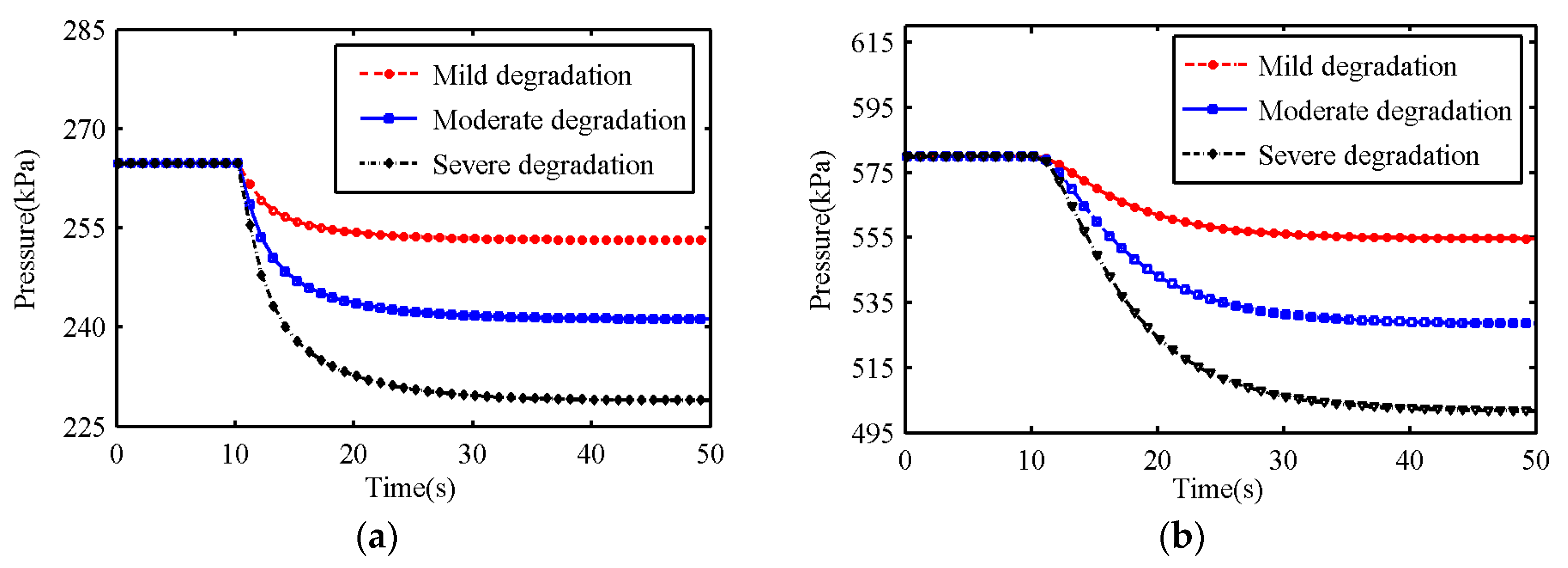
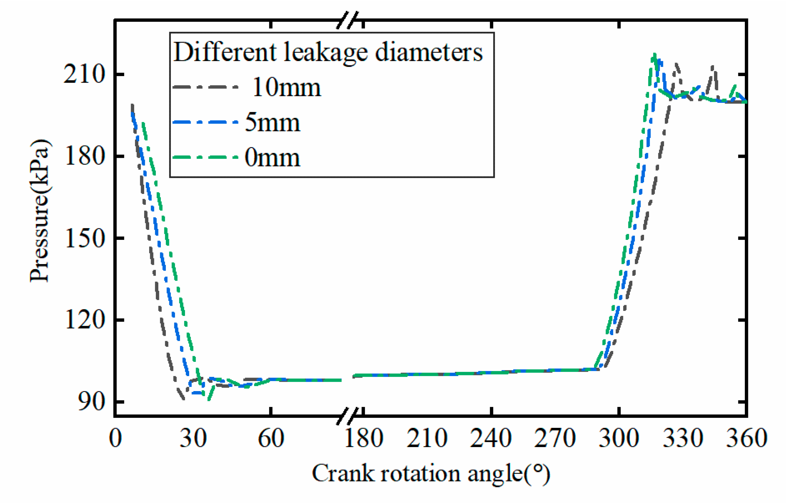
Nevertheless, investigating the field application of SCRS, the regulation failure and (or) performance degradation often occurred in long-term operation. The failure of capacity regulation extremely affected the safe and stable operation of the reciprocating compressor. According to statistics, there are many factors that affect the regulation performance of the system. The main factors and their effects are listed in

Table 1. The main factors that affect the regulation performance.

Factors	Location	Effect
reset spring stiffness	electro-hydraulic actuator	affects actuator withdrawal resulting in decreased precision or regulation failure
solenoid valve response	electro-hydraulic actuator	affects actuator withdrawal resulting in decreased precision or regulation failure
partial actuator failure	electro-hydraulic actuator	regulation accuracy decreases or fails
oil supply pressure too low	hydraulic system	fails to regulate
valve leakage	compressor	regulation accuracy decreases
controller failure	computer-controlled system	fails to regulation

. Among these factors, the most commonly encountered factors include valve leakage, deviation of the solenoid valve’s characteristics, and degradation of the unloader reset spring. An electro-hydraulic actuator is a high frequency action part, and its action frequency is directly related to the compressor speed. The high frequency action inevitably leads to the fatigue degradation of the reset spring of the unloader in long-term operation. The solenoid valve dynamic characteristics also offset due to continuous charging and discharging. Unfortunately, since the SCRS is a complex system with mechanical, electrical, and hydraulic coupling, the characteristic parameters of the reset spring and solenoid valve cannot be directly measured during system operation. Therefore, if there is a decrease in system regulation performance, it is extremely challenging, even impossible, to locate the fault through the technical method of single factor analysis.

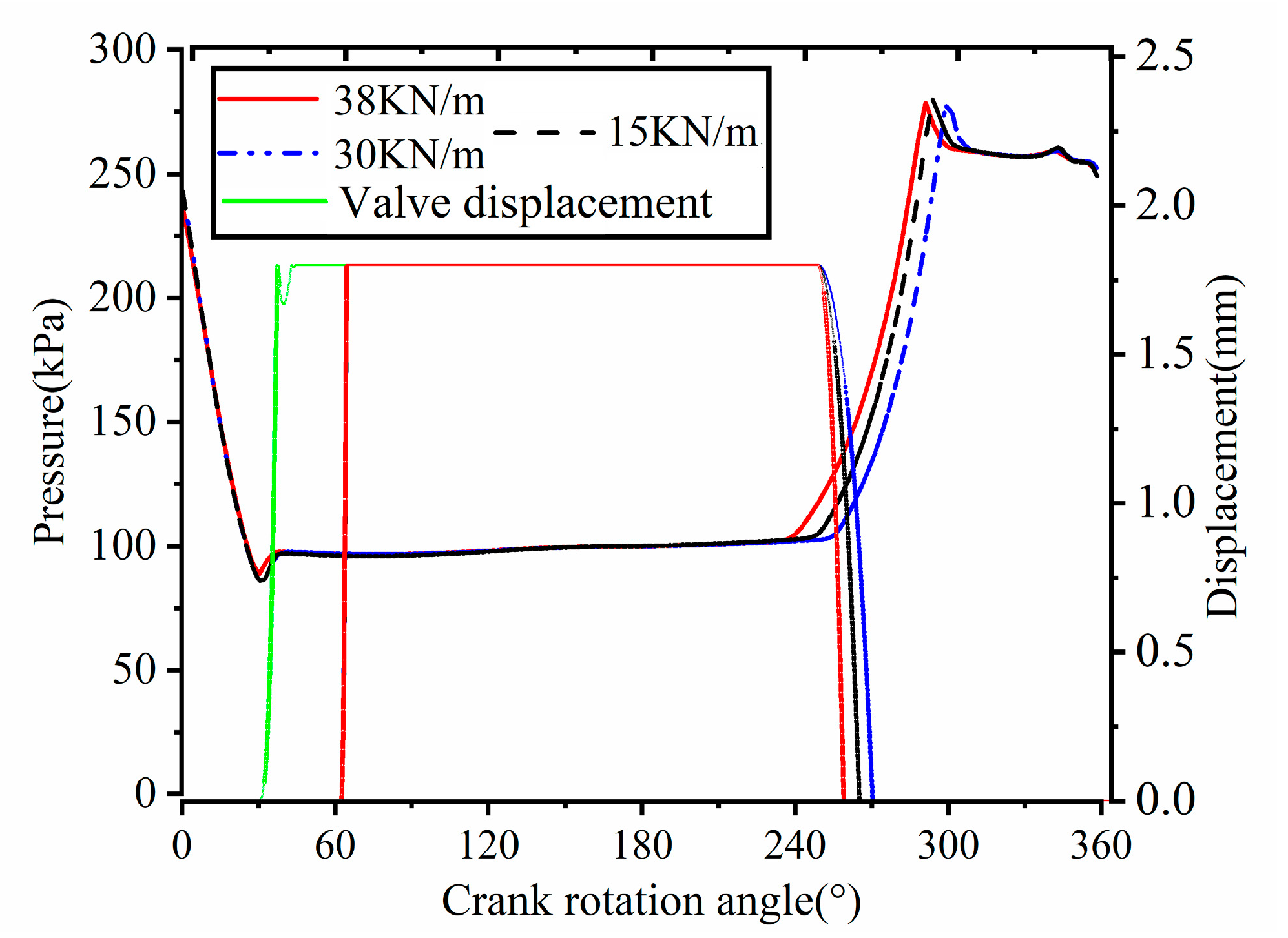
To address this issue, it is necessary to study the influence law between the system regulation performance and each coupling component and explore the degradation law of system performance caused by valve leakage, characteristic parameter deviation of the solenoid valve, and reset spring stiffness degradation. Therefore, this paper develops a multi-subsystem coupling model to analyze the relationship between the system regulation performance and the parameters of each component.

Some research has been done on system modeling. Liu et al. proposed a mathematical model that is coupled with a control system, hydraulic system, actuator, buffer tank, and other components [12]. However, the coupling model did not take the influence of the gas pipeline between compressor and buffer tank and the valve leakage into account. The opening and closing processes of the solenoid valve were also ignored. Based on the coupling multi-system model established in [12], an improved multi-subsystem integrated mathematical model, including compressor, gas pipeline, buffer tank, and actuator, was established, which took the solenoid valve dynamics and valve leakage into consideration.

Here, the framework of degradation-based optimization (DBO) was developed. The flow diagram of the developed DBO framework for SCRS is shown in Figure 1. In the operation of the SCRS, the load prediction model predicts the actual load of the compressor, and the degradation model calculates the degradation rate of the system based on the prediction results. At the initial time, the degradation rate of the system was very low and close to zero. With the degradation of the system’s regulating performance, the degradation rate gradually increased. The adaptive optimization compensation model generates control parameter compensation to compensate for the degraded part, which minimizes the degradation rate of the whole system and ensures the acceptable regulation accuracy and performance of the system.

The load prediction model is the most important part of the whole compensation-based optimization framework. Generally speaking, the load prediction model can be realized through mechanism modeling, but the mechanism model requires a large number of system structure parameters and process parameters which are not even measurable. Therefore, these models are unsuitable for engineering applications, especially in real-time control systems. Encouragingly, artificial neural networks (ANNs) have been widely used in reciprocating compressor modeling and system optimization due to their advantages of being adaptive, self-learning, and fault-tolerant and working with nonlinear mapping. Belman et al. set up a physical mechanism model and an artificial neural network model of a reciprocating compressor, respectively, with an experimental refrigeration device as the research object and analyzed and compared these models through parameters such as exhaust volume, exhaust temperature, and energy consumption [13]. Barroso-Maldonado et al. developed two models: one using an artificial neural network and another one using a probabilistic neural network to predict and simulate the behavior of a reciprocating compressor [14]. The artificial neural network models for the non-injection, vapor injection, and two-phase injection heat pumps were developed to predict the performance indexes during cooling and heating seasons [15]. An ANN was trained and validated with the experimental data and the same was proposed for the predicting performance of a work recovery scroll expander in closed-loop operation with a CO₂ refrigeration system in the sub-critical zone [16]. In addition, artificial neural networks are also widely used in parameter and system optimization. Mohammadi et al. assigned an ANN to investigate a logical interaction among dependent and independent variables and to define a cost function based on the empirical data; then the function was optimized by Genetic Algorithm to determine the best amount for each parameter [17]. A hybrid ANN model was trained as well as tested with experimental data sampled from statistical methods, and the model was used to predict the optimal process parameters of injection molding process of a bi-aspheric lens [18].

Hence, this study proposes an ANN-based model to predict the load of a compressor for evaluating the degradation rate of the SCRS. Although various methods have been developed to improve the prediction accuracy of ANN models, a back propagation (BP) neural network is still one of the most popular techniques in this field [19]. A gradient descent algorithm is usually used in a typical BP neural network. However, the typical BP neural network has the limitation of slow convergence speed and is easy to fall into a local extremum. As is well known, the particle swarm optimization (PSO) has the advantages of good global search capability and fast convergence speed. Therefore, PSO is used to optimize the initial connection weight and threshold of BP neural networks. Comparing an ANN model with and without PSO, the prediction error of an ANN model with PSO is lower than without using PSO. Since the optimization is a steady-state optimization, an adaptive optimization method based on the degradation rate is proposed to avoid the over-optimization caused by the load prediction error.

In this work, a multi-subsystem coupling mathematical model including compressor, gas pipeline, buffer tank, actuators, and other components is developed to study the performance degradation law of the SCRS caused by changes in the actuator’s dynamic characteristic parameters and valve leakage. Then the degraded performance of the SCRS is optimized based on the developed DBO framework. The objective of performance optimization is to minimize the degradation rate of the SCRS. The key outcomes resulting from the proposed DBO framework are the control parameter compensation which leads the SCRS to operate at minimum degradation rate and to guarantee acceptable regulation accuracy. The effectiveness of the proposed DBO framework was verified by the implementation results.

This paper is organized as follows: Section 2 introduces the composition and working principle of the SCRS. Section 3 describes the multi-subsystem coupling model. The law of performance degradation is analyzed in Section 4. Section 5 provides the load prediction model based on improved PSO-BP and proposes an optimization method. The model prediction accuracy and implementation results of the proposed optimization method are also discussed in Section 5. Finally, Section 6 concludes the paper.

2. System Description

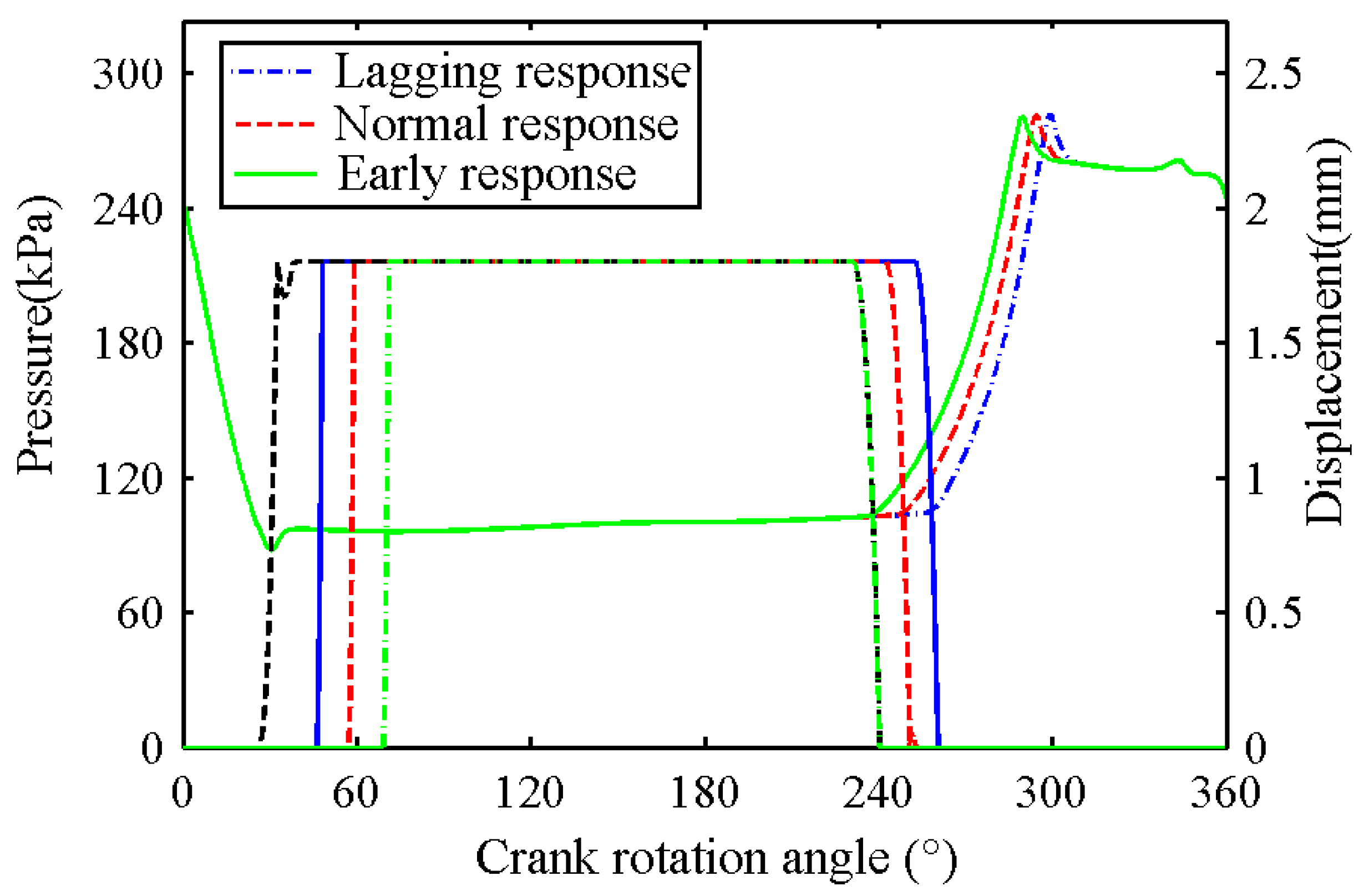
The basic principle of capacity regulation of a reciprocating compressor is that the movement of the suction valve is controlled by external forces which delay its closure [6]. A part or all of the gas in the cylinder flows back to the inlet line before it is compressed, and only the required gas is compressed. The power consumption and actual volume gas are directly proportional [1]. Therefore, the power consumption of the compressor is reduced when it is not under full load.

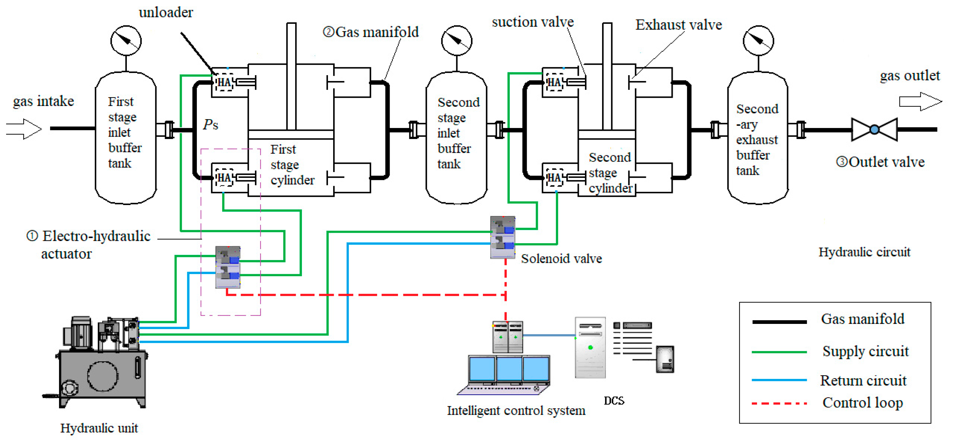
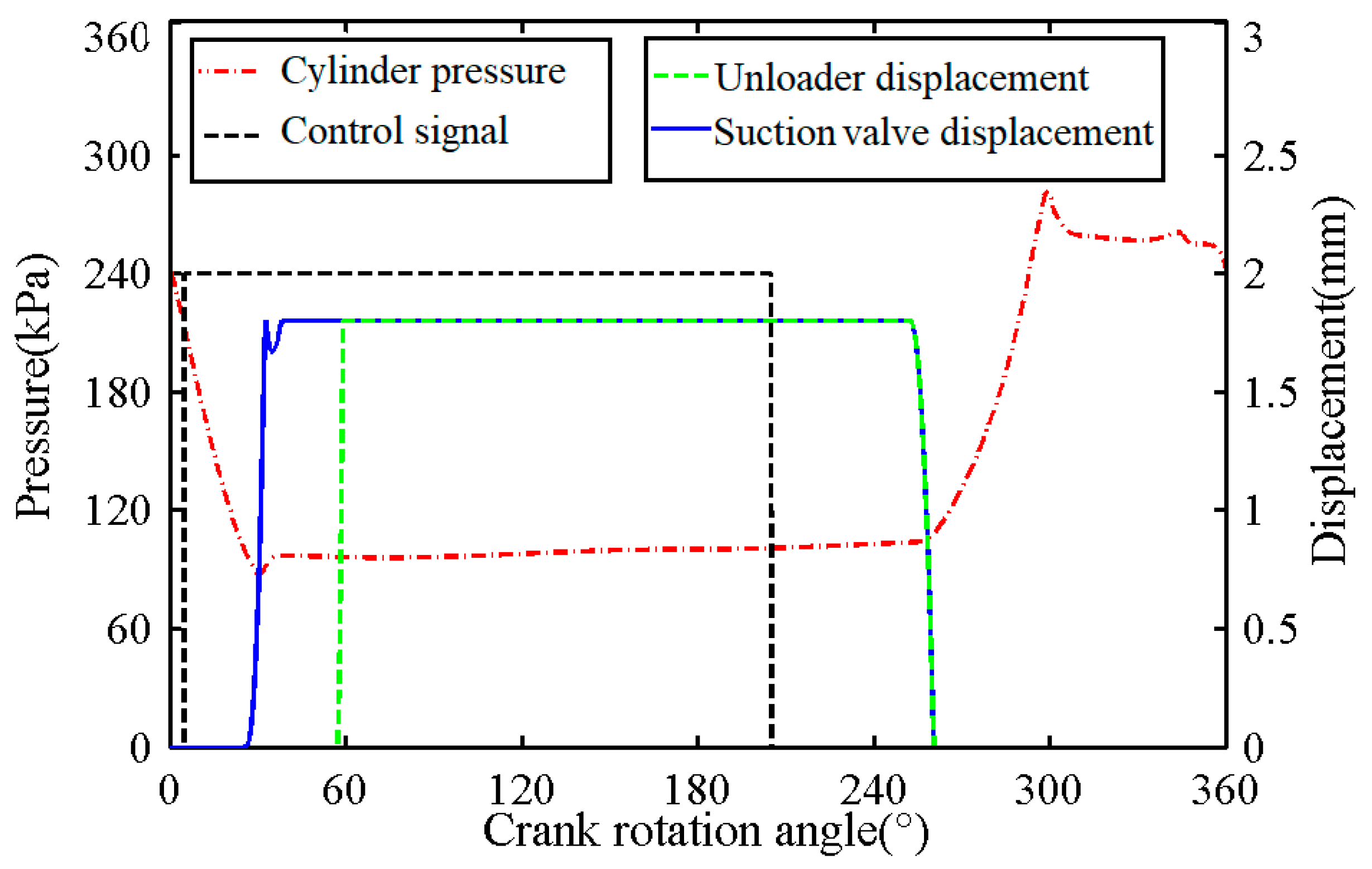
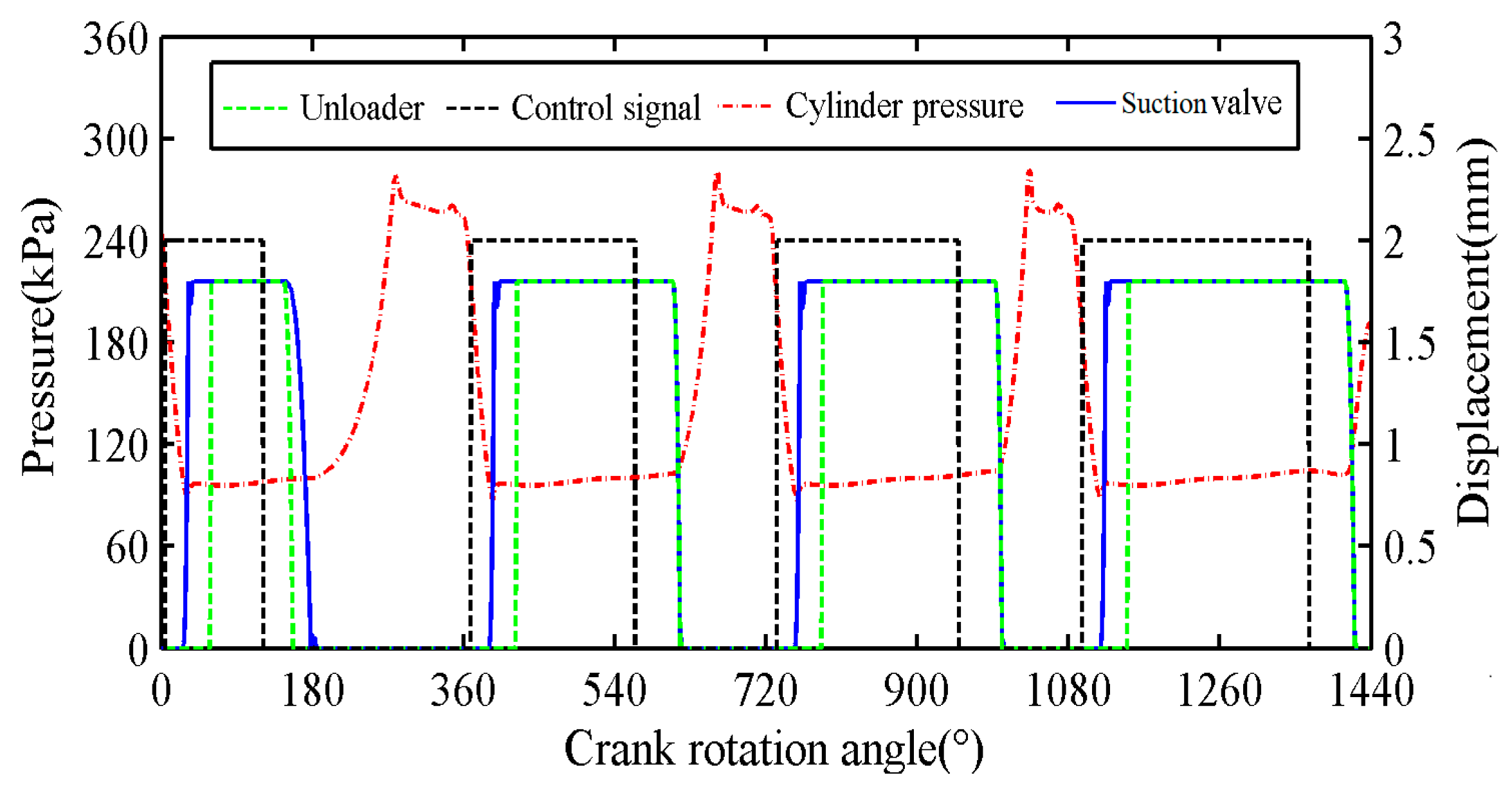
The reciprocating compressor pressure system with SCRS can be called the variable capacity reciprocating compressor pressure system (VCRCPS). The VCRCPS consists of a reciprocating compressor, buffer tanks, an outlet valve, and a SCRS which is integrated with a hydraulic system, an intelligent control system, and an electro-hydraulic actuator, as shown in Figure 2. The gas is compressed by a reciprocating compressor to realize a pressure boost. The hydraulic system provides the hydraulic driving force. The intelligent control system records the exhaust pressure, temperature, and the signal of the top dead center (TDC) of the compressor to calculate the load and output-corresponding control signal. The electro-hydraulic actuator responds according to the control signal to make part of the gas return into the inlet line without compressing, so as to realize capacity regulation.

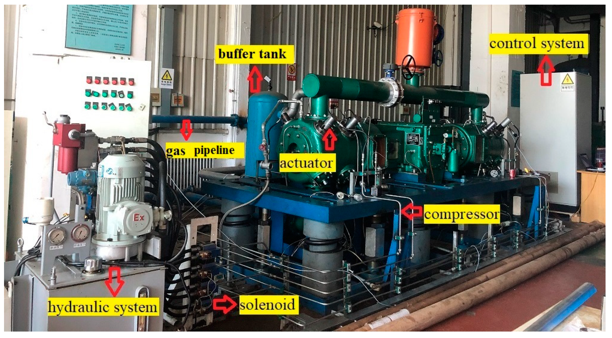
The object studied in this paper is a two-stage reciprocating compressor with SCRS, as shown in Figure 3, including a control system, hydraulic system, gas pipeline, buffer tank, electro-hydraulic actuator, etc. The main operating parameters are listed in

Table 2. Operation parameters of the compressor and the SCRS.

Item	Value
Rated speed (r/min)	300
Stage number	2
Number of cylinders	2
Buffer tank capacity (m3)	0.3/0.16
Spring stiffness (kN/m)	38
Hydraulic pressure (MPa)	7
Suction pressure (kPa)	101
Exhaust pressure (kPa)	27/700
Exhaust volume (m3/min)	12
Number of suction valves	4/4
Number of exhaust valves	4/4

.

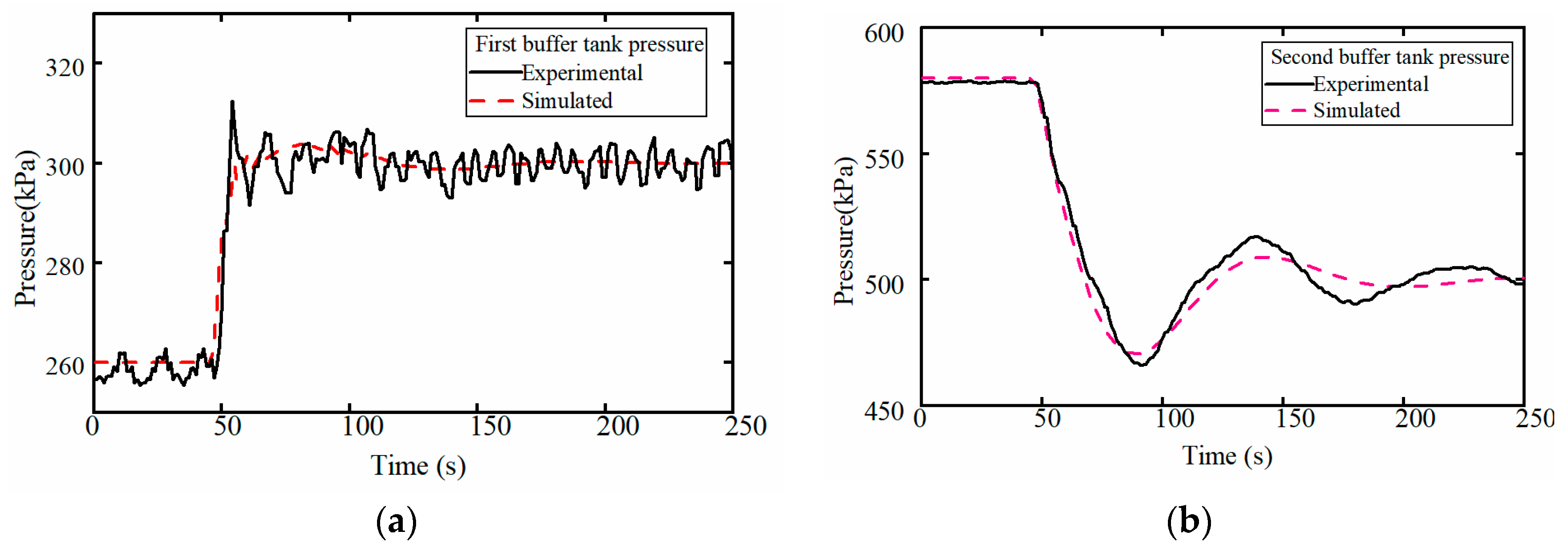
The load regulation experiments were carried out on the test bench to verify the modified multi-subsystem mathematical model. The performance optimization method proposed in this paper was also verified on this test bench.

3. Mathematical Model

This section summarizes the mechanism mathematical model to describe the dynamic characteristics and analyze the effects of valve leakage and actuator parameter changes on the SCRS performance. For this, modeling of all subsystems is presented below.

3.1. Compressor

In order to establish the mechanism’s mathematical model of the compressor, some basic assumptions were made for the working process of the compressor:

• Ideal homogeneous medium is in the cylinder, that is, the pressure, temperature, and density are the same at any two points of the medium;
• The flow process of gas in and out of the cylinder is adiabatic and stable;
• Energy transfer in the working cylinder is uniform.

The chamber of the compressor is taken as a control volume, and the inlet valve leakage is considered. It is modelled as an additional flow through an orifice in parallel to the normal valve flow [20]. The equation for the cylinder pressure $P_{cy}$ can be derived from the continuity and the first law of thermodynamics as

$$\frac{d{p}_{cy}}{d\theta }=\frac{1}{V_{cy}\left(\theta \right)}\left(\begin{array}{l}{c}_i^2\frac{d{m}_{cin}}{d\theta }-c_{{}_{cy}}^2\frac{d{m}_{cd}}{d\theta }-\gamma p_{cy}\frac{d{V}_{cy}}{d\theta }-\\ c_i^2\frac{d{m}_{iL}}{d\theta }-c_{{}_{cy}}^2\frac{d{m}_{dL}}{d\theta }\end{array}\right),$$

(1)

where the instantaneous volume of the cylinder $V_{cy}(\theta )$ and its change rate $\frac{d{V}_{cy}}{d\theta }$ can be calculated by the clearance volume and piston motion, respectively.

$$V_{cy}(\theta )=V_{c0}+S_{cy}{x}_{cy}(\theta ),$$

(2)

$$\frac{d{V}_{cy}(\theta )}{d\theta }=S_{cy}\frac{d{x}_{cy}(\theta )}{d\theta },$$

(3)

where $\theta =\omega t$ represents the rotation angle of the crankshaft relative to the top dead center. $\frac{d{m}_{cin}}{d\theta }$ and $\frac{d{m}_{cd}}{d\theta }$ are the mass flow through the inlet and discharge valves, respectively. $\frac{d{m}_{iL}}{d\theta }$ and $\frac{d{m}_{dL}}{d\theta }$ are the mass flow rate of inlet and discharge valve leakage, respectively. $\gamma$ = 1.4 is the ratio of specific heats. $c_i{}^2=\gamma R{T}_i$ is the squared speed of sound in the inlet chamber. $c_{{}_{cy}}^2=\gamma R{T}_{cy}$ is the squared speed of sound in the cylinder. $V_{c0}$ is the clearance volume. R is the gas constant.

In full load condition, inlet and discharge valves of the reciprocating compressor are automatic valves. For the inlet valve, the driving force is the difference value between the suction pressure and the gas pressure in the cylinder. However, the additional force provided by the hydraulic system acts on the valve plate under the regulation condition. The movement of the suction valve plate can be described as:

$$M_{sv}{\omega }^2\frac{d^2{x}_{sv}}{d{\theta }^2}+c_{ss}\omega \frac{d{x}_{sv}}{d\theta }+k_{sv}{x}_{sv}-F_{hu}={\displaystyle \sum f_{sv}},$$

(4)

where $F_{hu}$ is the additional hydraulic force; $M_{sv}$ represents the total equivalent motion mass of suction valve and actuator; $\frac{d^2{x}_{sv}}{d{\theta }^2}$, $\frac{d{x}_{sv}}{d\theta }$, and $x_{sv}$ are the valve plate acceleration, velocity, and displacement, respectively; $c_{ss}$ is the damping coefficient; ${\displaystyle \sum f_{sv}}$ represents the resultant force on the valve which is from three forces: gravity of valve, the preset force, and differential pressure force; and $k_{sv}$ is equivalent spring stiffness.

The mass flow rate through the inlet valve and discharge valve can be expressed as Equations (5) and (6), respectively.

$$\frac{d{m}_{cin}}{d\theta }=C_i{A}_{fs}\frac{1}{\omega }\sqrt{2{\rho }_{cy}|p_i-p_{cy}|},$$

(5)

$$\frac{d{m}_{cd}}{d\theta }=C_d{A}_{fd}\frac{1}{\omega }\sqrt{2{\rho }_{cy}|p_d-p_{cy}|},$$

(6)

where $A_{fs}$ is the maximum flow area of all inlet valves; $p_i$ and $p_d$ represent the suction and exhaust pressures, respectively; $A_{fd}$ is the maximum flow area of all discharge valves; ${\rho }_{cy}$ is the density of the gas in the cylinder; $C_d$ is a variable discharge coefficient which accounts for the reduced flow area resulting from the separated flows and changes with the valve lift; and $C_i$ is a variable suction coefficient. The mass flow rate of inlet and discharge leakage can also be calculated according to Equations (5) and (6) by using the leakage flow area instead of the flow area of valve. In this study, the influence of leakage on the capacity regulation effect is studied.

3.2. Gas Pipeline

The gas pipeline is mainly connected to the exhaust chamber, exhaust buffer tank, separator, heat exchanger, and the inlet buffer tank of the next stage. For the gas pressure and temperature in the gas pipeline, the polytropic equation is used for modeling analysis. The gas pipeline model is shown in Figure 4. The pipeline length is assumed to be L and the pipe diameter to be D. In the gas pipeline, the mass flow equation of gas is given by [21].

$${\dot{m}}_{tout}(q,L,t)=\{\begin{array}{cc}0& if\hspace{1em}t<L/c\\ e^{-\frac{R_{t}RT}{2p}\frac{L}{c}}q(t-\frac{L}{c})& if\hspace{1em}t\ge L/c\end{array},$$

(7)

where ${\dot{m}}_{tout}(q,L,t)$ represents the mass flow rate flowing out through the gas pipeline, $q(t)$ represents the inlet flow of pipeline, $R_t$ is the pipeline impedance, $c$ is the airflow speed in the gas pipeline, and P and T represent the inlet pressure and temperature, respectively.

3.3. Electro-Hydraulic Actuator

The electro-hydraulic actuator is a key part of the SCRS, which consists of a mechanical unloader, a hydraulic cylinder, and a high-speed solenoid valve. When the regulating system is working, the high-pressure hydraulic oil flows into and out of the hydraulic cylinder through the high-speed solenoid valve and controls the extension and retraction of the mechanical unloader.

The dynamic response performance of the solenoid valve has a great influence on the system’s performance. The dynamic performance of the solenoid valve mainly includes four parts: opening delay, opening moving time, closing delay, and closing moving time. If the excitation voltage is fixed, the supply hydraulic pressure has little effect on the opening delay and opening moving time, but it has a great influence on the closing delay and closing moving time [22]. Hence, the dynamic performance of the solenoid valve is determined and can be obtained by model calculation or experimental test, as mentioned in the literature [22].

In order to simplify the mathematical model of the electro-hydraulic actuator, the opening and closing processes of the solenoid valve are simplified. The opening delay, opening moving time, closing delay, and closing moving time are $t_1$, $t_2$, $t_3$, and $t_4$, respectively. The solenoid valve control port flow area can be expressed on the time axis of a single operation cycle T of the compressor as follows.

$$A\left(t,t_c\right)=\{\begin{array}{cc}{A}_h& t_{on}\le t\le t_c+t_{off}\\ 0& otherwise\end{array},$$

(8)

where $t_{on}=t_1+t_2/2$ is the equivalent opening delay of the solenoid valve. Similarly, $t_{off}=t_3+t_4/2$ represents the equivalent closing delay of the solenoid valve. $t_c$ is the hold time of switching on the control signal output from the solenoid valve driver.

The dynamic characteristic model of the electro-hydraulic actuator can be expressed as follows.

$$\{\begin{array}{l}{Q}_h(u)=C_h{A}_h\left(t,t_c\right)\sqrt{\frac{2(P_{oil}-P_A)}{{\rho }_{oil}}+C_h{\tilde{A}}_h\left(t,t_c\right)\sqrt{\frac{2}{{\rho }_{oil}}{P}_A}}\\ Q_h(u)=A_A\dot{x}+C_l{P}_A\\ \\ F_{hu}=P_A{A}_A-K_f\left(x+x_0\right)=m_A\ddot{x}+B\dot{x}\end{array},$$

(9)

where $Q_h$ represents the hydraulic fluid flow of the control port of the high-speed solenoid valve, $C_h$ represents the flow coefficient, $P_{oil}$ represents the supply pressure, $P_A$ represents the pressure in the hydraulic cylinder, ${\rho }_{oil}$ represents the hydraulic oil density, $A_A$ represents the piston area of the oil cylinder, $x$ is the load displacement, $C_l$ is the oil cylinder leakage coefficient, B represents the cylinder damping coefficient, $x_0$ represents the pre-compression amount of the loaded spring, $m_A$ represents the equivalent mass of the cylinder piston and load, and $K_f$ represents the reset spring stiffness of the unloader, which is an extremely important parameter that has a great impact on the regulation effect, but it is also a component that easily degrades. Therefore, the influence of the reset spring stiffness is thoroughly analyzed in the following Section 4.

At a certain time, the switch-off control signal output is sent from the solenoid valve driver. The hydraulic force is released, and the mechanical unloader is lifted up by the spring force. Then all the suction valves will close together with the mechanical unloader. The hold time $t_c$ is determined by the compressor load ratio η, as indicated below [10].

$$\eta V_s+V_{exp}+V_{cle}=V_{cle}+V_{str}\left(1-cos{\theta }_r+\frac{\lambda }{2}{sin}^2{\theta }_r\right),$$

(10)

$$t_c=30{\theta }_r/n\pi -t_{off}-t_0,$$

(11)

where n represents compressor speed, ${\theta }_r$ is the inlet valve plate closing angle, and $t_0$ is a constant dependent on where the actuator is extended. The influence of parameters $t_{on}$ and $t_{off}$ on the system regulation effect is analyzed in Section 4.

3.4. Outlet Valve

The final exhaust buffer tank of the reciprocating compressor is connected with the process pipeline through a one-way valve. When the pressure of the buffer tank is greater than the pressure behind the valve, the gas in the buffer tank is vented outward through the one-way valve. The standard equation for the mass flow through an orifice of an area $A_v$ is [21]:

$${\dot{m}}_v\left(P_u,P_d\right)=\{\begin{array}{l}{C}_f{A}_v{C}_1\frac{P_u}{\sqrt{T}}\begin{array}{cc}& if\frac{P_d}{P_u}\end{array}\le P_{cr}\\ C_f{A}_v{C}_2\frac{P_u}{\sqrt{T}}{\left(\frac{P_d}{P_u}\right)}^{1/k}\sqrt{1-{\left(\frac{P_d}{P_u}\right)}^{\left(k-1\right)/k}}\begin{array}{cc}& if\end{array}\frac{P_d}{P_u}>P_{cr}\end{array},$$

(12)

where ${\dot{m}}_v$ is the mass flow through the valve orifice; $P_u$ and $P_d$ represent the upstream pressure and the downstream pressure, respectively; k is the specific heat of an ideal gas; and C₁ and C₂ are constants for a given fluid. For air (k = 1.4), we have $C_1$ = 0.040418, $C_2$ = 0.15617, and $P_{cr}$ = 0.528. $C_f$ is a non-dimensional discharge coefficient which is generally in the range of 0.8–0.85.

3.5. Buffer Tank

Considering the control volume V with a density ρ, mass m, pressure P, and temperature T, the time derivative of the chamber pressure can be obtained by using three important equations: the equation of state (ideal gas) law, the conservation of mass equation, and the energy equation. The unified form of the dynamic pressure equation in the control volume is Equation (13). The detailed derivation process can be seen in [21].

$$\dot{P}=\frac{RT}{V}\left({\alpha }_{in}{\dot{m}}_{in}-{\alpha }_{out}{\dot{m}}_{out}\right)-\alpha \frac{P}{V}\dot{V},$$

(13)

where $\alpha$, ${\alpha }_{in}$, and ${\alpha }_{out}$ represent the coefficients of gas inflow and outflow, whose value depends on the heat transfer process in the actual process, and their values range are between 1 and k.

The volume of the inlet and exhaust buffer tank is fixed, and the gas in the tank can fully exchange heat with the outside through the pipe wall, which can be approximately regarded as an isothermal process, namely ${\alpha }_{in}$ = ${\alpha }_{out}$ = 1. The pressure of the buffer tank can be expressed as:

$${\dot{P}}_{buff}=\frac{RT}{V_{buff}}\left({\dot{m}}_{in\_buff}-{\dot{m}}_{out\_buff}\right),$$

(14)

where, ${\dot{P}}_{buff}$ represents the change of pressure in the buffer tank, $V_{buff}$ represents buffer tank volume, and ${\dot{m}}_{in\_buff}$ and ${\dot{m}}_{out\_buff}$ represent the gas mass flow into and out of the buffer tank, respectively.

3.6. Overall Model

The pipeline length between the first-stage cylinder and inter-stage buffer tank is L₁. The pipeline length between the second-stage cylinder and inter-stage buffer tank is L₂. The pipeline length between the secondary cylinder and the exhaust buffer tank is L₃. The back pressure behind the outlet valve of the second-stage exhaust buffer tank is $P_{dd}$, and the volumes of the first-stage buffer tank and the second-stage buffer tank are V₁ and V₂, respectively.

Combining Equations (1)–(14), the multi-system coupling mathematical model of the two-stage compressor is introduced below.

$$\{\begin{array}{l}{\dot{P}}_1=\frac{R{T}_1}{V_1}\left({\dot{m}}_{1out}({\dot{m}}_{cd1},L_1,t)-{\dot{m}}_{2in}({\dot{m}}_{c1n2},L_2,t\right)\\ {\dot{P}}_2=\frac{R{T}_2}{V_2}\left({\dot{m}}_{2out}({\dot{m}}_{cd2},L_3,t)-{\dot{m}}_v(P_2,P_{dd})\right)\end{array},$$

(15)

where P₁ and P₂ represent the pressure of the first-stage exhaust buffer tank and the second exhaust buffer, respectively.

4. System Simulation and Performance Analysis

The model simulation was performed in a MATLAB/SIMULINK environment. The dynamic characteristics of the system and the key parameters that affect the system regulation performance were analyzed. The key structural parameters of the models are shown in Table 2.

4.1. Model Validation and Dynamic Characteristics of SCRS

Under full load condition, four operating processes were completed in one cycle of the compressor, namely suction, compression, discharge, and expansion. Under part-load conditions, a reverse stroke followed after the suction process [10]. The movement of the suction valve plate was changed by the actuator when the capacity regulation system was operated. The movement of the actuator was determined by the hydraulic pressure and the reset spring force, which influenced the working process of regulation system.

The measured and predicted cylinder pressure in one cycle of the compressor under three typical load conditions (100%, 70%, 40%) is shown in Figure 5. A step decrease was designed for the first-stage load ratio (80–60%) and the second-stage load ratio (80–50%) at 50 s, respectively. The change of the buffer tank pressure is shown in Figure 6. Compared with the measured results, the simulation results exhibit good consistency over different load conditions. The results verify that the presented model is acceptable and valid.

The relationship among the control signal (60% load), the displacement of the suction valve plate, the displacement of actuator, and the pressure in cylinder with a crank angle under the capacity regulation condition is shown in Figure 7. It can be clearly seen that the delay from the high-level control signal to the start of the movement of the unloader is about 50° caused by the opening delay of the solenoid valve, and the moving time of the unloader is about 6°. The delay from the low-level control signal to the start of the reset of the unloader is about 47° caused by the closing delay of the solenoid valve, and the reset action time of the unloader is about 12°.

In order to study the influence of the control parameter characteristics on the system’s dynamic performance and controllability [23], different loads and a different exhaust flow were realized by changing the duty cycle of the control signal. As shown in Figure 8, when the duty cycle of the control signal was too low (less than 30%), the unloader reset before the compression process started, and the valve plate reset automatically. Hence, the cylinder was working at full load, and the exhaust flow was not adjusted. When the duty cycle was large enough (greater than 75%), the suction valve plate could not be withdrawn during the whole operation cycle of the compressor, all gas was returned, nothing was compressed, and the exhaust flow of the compressor was zero.

4.2. Performance Degradation Analysis

The regulating performance of the SCRS is mainly affected by the dynamic characteristics of the electro-hydraulic actuator (including the reset spring and the dynamic characteristics of the solenoid valve) and the running state of the valve. If the dynamic characteristic of the electro-hydraulic actuator changes or there is valve leakage, the system regulation performance will degrade and even cause capacity regulation failure. Therefore, this section analyzes the degradation law of system regulation performance.

4.2.1. Effect of Reset Spring

The actuator performance degrades due to wear and aging in the long running process. Especially, the stiffness of the reset spring in the actuator changes greatly due to fatigue caused by the repetitive duty cycle, which affects system regulation accuracy. Hence, the system dynamic characteristics and the variation law of the buffer tank pressure under different degradation degrees of the reset spring stiffness were studied.

The reset spring acts as the reverse force in the ejection process of the actuator and as the driving force in the reset process of the actuator. Combined with the oil supply pressure, the limit of the withdrawal speed of the actuator, and the inlet pressure, the optimal design stiffness of the low-pressure stage reset spring can be calculated, and its value is 38 kN/m. Figure 9 indicates that the change of spring stiffness mainly affected the reset process of the valve plate but had no effect on the opening process of the valve plate. The greater the spring stiffness was, the shorter the reset time. The response times of the valve plate were 12° (6.6 ms), 18° (10 ms), and 24° (13 ms) when the reset spring stiffness was 38 kN/m, 30 kN/m, and 15 kN/m, respectively.

Figure 10 displays the pressure change rules of both the first-stage exhaust buffer tank and the second-stage exhaust buffer tank, respectively, when the spring stiffness of the high-pressure stage actuator is normal, and the spring of the low-pressure stage actuator has different degradations (slight degradation: 38 kN/m–30 kN/m; moderate degradation: 38 kN/m–25 kN/m; severe degradation: 38 kN/m–15 kN/m). The first-stage load and second-stage load were set as 85% and 80%, respectively. Under normal regulation conditions, the pressure of the first-stage exhaust buffer tank was 264 kPa, and the pressure of the second-stage exhaust buffer tank was 580 kPa. When the spring of the low-pressure stage actuator degenerated, both the pressure of the first-stage exhaust buffer tank and the pressure of the second-stage exhaust buffer tank decreased significantly. The more the spring degraded, the more the pressure dropped. The exhaust buffer tank pressure in stable state under different stiffness values is summarized in

Table 3. The pressure varies with the stiffness of the spring.

Spring Stiffness	First Stage Buffer Tank Pressure	Second Stage Buffer Tank Pressure
38 kN/m	264 kPa	580 kPa
30 kN/m	253 kPa	555 kPa
25 kN/m	241 kPa	542 kPa
15 kN/m	230 kPa	508 kPa

. As can be seen from the table, the spring stiffness changed from the design value of 38 kN/m to 15 kN/m, and the pressure of the first- and the second-stage exhaust buffer tank decreased by 34 kPa and 72 kPa, respectively. It means that the actual control load decreased with the degeneration of the spring. Therefore, it is conceivable that capacity regulation will fail if the reset spring stiffness degrades severely.

4.2.2. Effect of Solenoid Valve Performance Parameters

The solenoid valve is an important part of the electrohydraulic actuator. The dynamic characteristics of the high-speed solenoid valve have a significant effect on the action characteristics of actuator. There are many influencing factors in its dynamic change [11]. This paper does not discuss the factors that affect the dynamic response of the high-speed solenoid valve but only the influence of the dynamic response of the high-speed solenoid valve on system capacity regulation performance.

The influence of the dynamic response of the solenoid valve on the dynamic process of the suction valve plate, and the dynamic pressure in the cylinder is illustrated in Figure 11. The dynamic characteristics of the solenoid valve affect both the actuator’s extension and retraction movements.

The high-pressure stage actuator was normal, and the solenoid valve response of the low-pressure stage actuator with different degree changes of response is shown in Figure 12. The load of the first stage and the second stage were both set as 80%. Under normal regulation conditions, the pressure of the first and second exhaust buffer tanks were 270 kPa and 533 kPa, respectively. The pressure variation of the buffer tank under different solenoid valve responses is shown in

Table 4. Buffer tank pressure variation under different responses of the solenoid valve.

Change in Response	First-Stage Buffer Tank Pressure	Second-Stage Buffer Tank Pressure
0 ms	270 kPa	533 kPa
3 ms	262 kPa	545 kPa
5 ms	253 kPa	555 kPa
8 ms	245 kPa	563 kPa

.

When the solenoid valve responded 8 ms in advance of the normal response, the pressure of the first-stage exhaust buffer tank was reduced by 25 kPa, and the pressure of the second-stage exhaust buffer tank was increased by 30 kPa. Therefore, if the solenoid valve changed in response, the accuracy of the capacity regulation decreased under the original design parameters. If the response changes greatly, control instability will be caused, which will affect the safe and stable operation of the compressor.

4.2.3. Effect of Valve Leakage

In addition to the system components’ characteristic parameter change, the compressor valve’s working state also has a certain influence on the capacity regulating effect.

Figure 13 displays the pressure in the cylinder with different suction valve leakage diameters when the compressor was fully loaded. As can be seen from the figure, the expansion process decreased and the suction valve plate was opened in advance caused by the leakage of the suction valve. A larger leakage resulted in the expansion process to occur earlier and consequently introduced a larger loss of discharge efficiency. The compression process increased, and the discharge process decreased due to the leakage of high-pressure gas from the cylinder, which is equivalent to the reduction of the actual capacity of the compressor. When the diameter of the leakage orifice of the suction valve is increased from 3 to 7 mm, the angle at the end of the expansion process is advanced by 3°, and the angle at the beginning of the exhaust process is delayed by 5°.

Under 40% load regulation condition, the comparison of the pressure curves in the leakage holes of the suction valves with different diameters is shown in Figure 14. The angle at the end of the expansion process is advanced from 35° to 25°, and the angle at the beginning of the exhaust process is delayed from 315° to 327° when the diameter of the leakage hole of the suction valve changed from 0 to 10 mm. In order to further analyze the influence of the leakage on capacity regulation, the changing trend of the ratio between the area of the indicator diagram with different leakage diameters and the area of the indicator diagram without leakage at full load is shown in Figure 15. It can be seen that the capacity control effect was larger than the design value caused by the suction valve leakage.

It can be concluded from the above analysis that the reset spring of the unloader, the performance parameters of solenoid valve, and valve leakage will all cause system regulation performance degradation and decrease the regulation accuracy. It also indicates that the same control signal will generate different regulation results if the operation parameters are different. To address this problem, it is necessary to evaluate and optimize the system performance in real time to ensure the accuracy and performance of the system.

5. Prediction Modeling and System Optimization

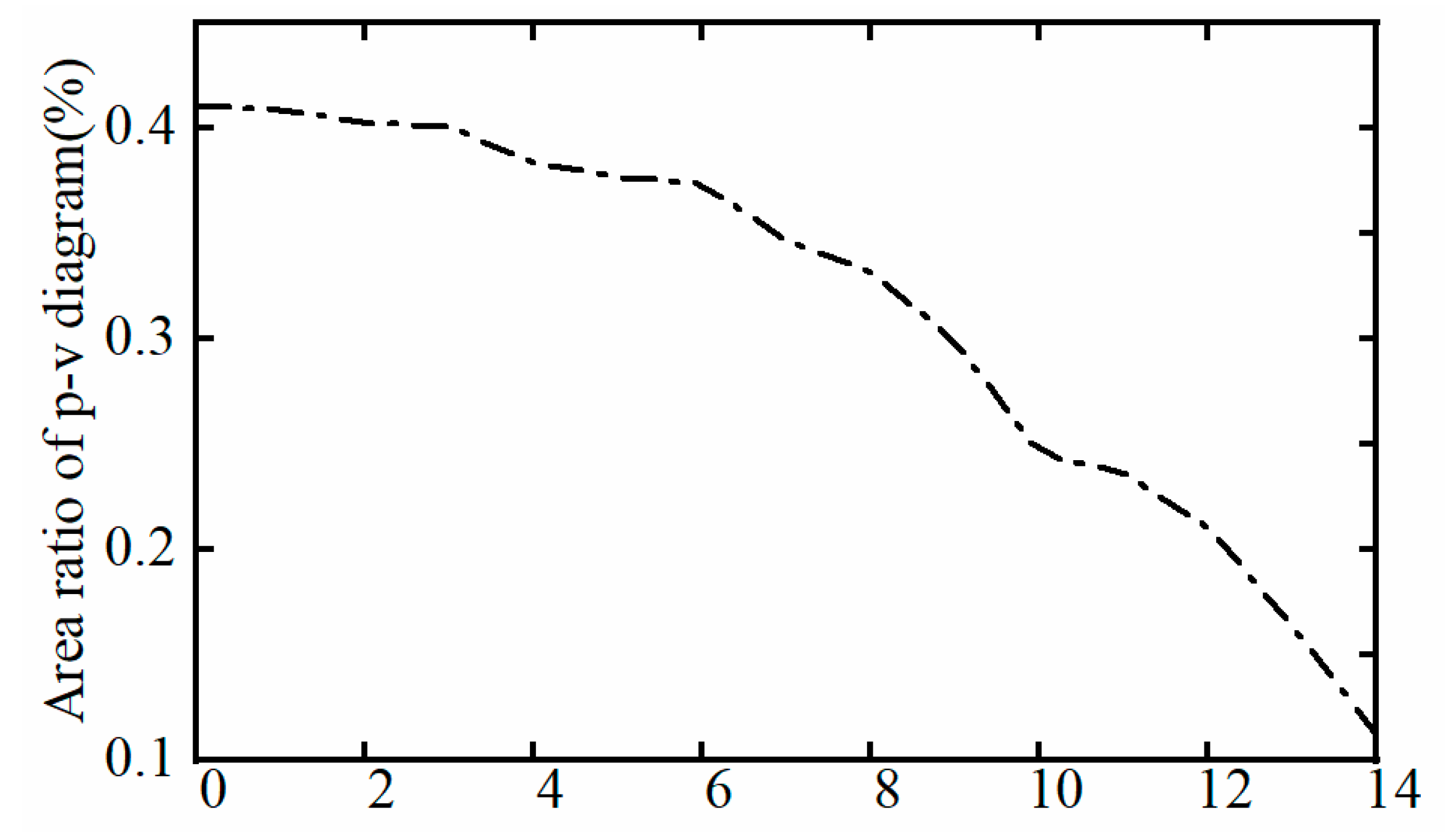
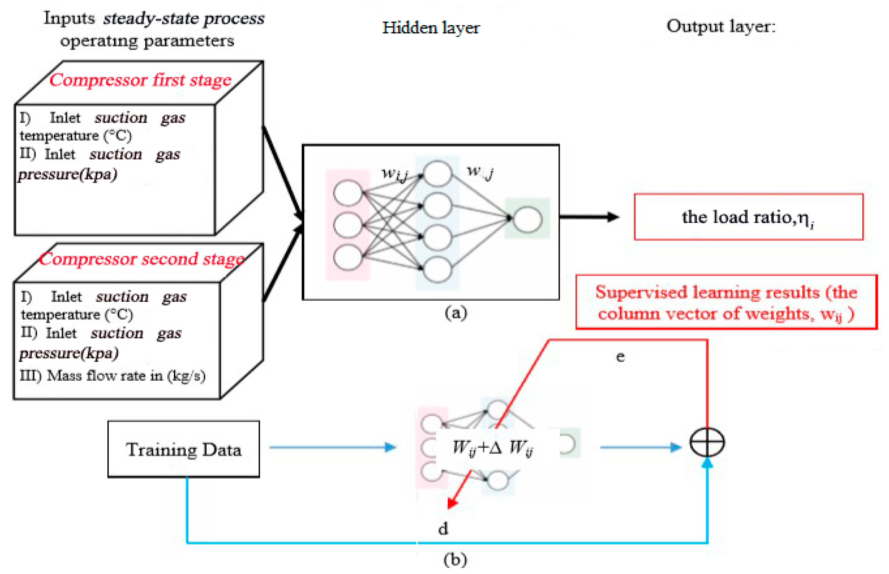
Fortunately, by studying the dynamic characteristics and the degradation law of the system and combining the actual operation experience, it is found that there are corresponding relations among exhaust flow, inlet and outlet pressure, inlet temperature, and compressor load. The load prediction model can be constructed by using the inlet and outlet pressure $P_i$, the inlet and outlet temperature $T_i$, and the exhaust flow Q. Under capacity regulation condition, the performance of the SCRS can be predicted, and the estimated value ${\tilde{\eta }}_i$ of the actual operating load of the cylinder can be obtained. Through the estimated value of the load ${\tilde{\eta }}_i$, the control parameters of the SCRS can be optimized online.

5.1. Load Predicting Model

A BP neural network is an artificial neural network based on a back-propagation learning algorithm, which is the main component of an artificial neural network [24]. Most of the existing BP neural network models are variations or improvements of the standard BP neural network model. In this study, the improved PSO-BP neural network is used to build the load prediction model. 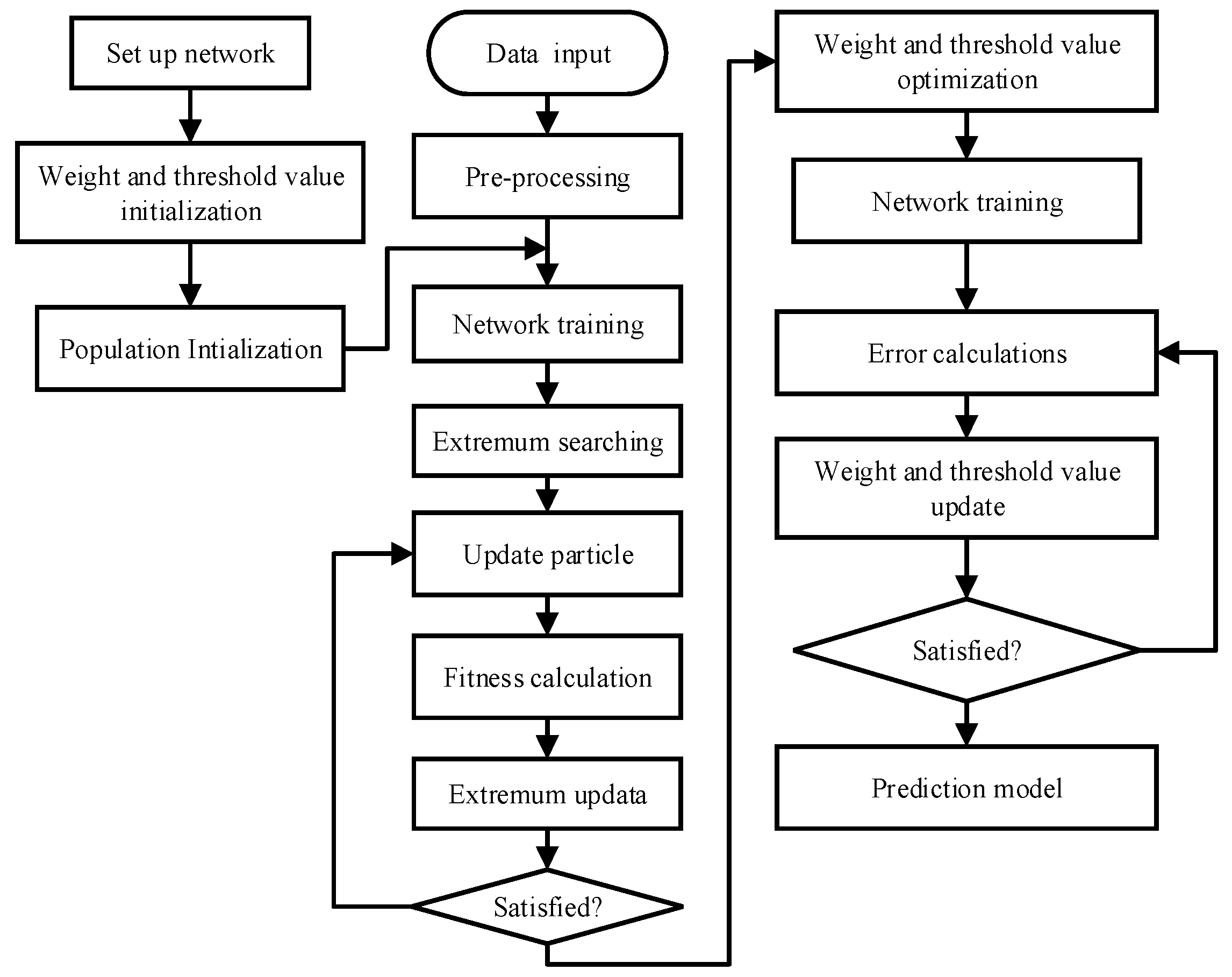The structure of the prediction model is illustrated in Figure 16. The initial thresholds and weights of the BP neural network are obtained through PSO optimization. Then the improved BP neural network is trained. The flow chart is plotted in Figure 17.

The particle swarm optimization (PSO) algorithm presents an efficient technique for solving optimization problems, especially the problem of a non-differentiable function where it is hard to find the optimum. PSO is a swarm intelligence algorithm inspired by the foraging behavior of birds. The position and the velocity of the population members are calculated by using a mathematical operator so they can be expected to head toward the best solution. The updating operation is defined as follows:

$$\begin{array}{c}{V}_i\left(k+1\right)=\omega \left(k\right)V_i\left(k\right)+c_1{r}_1\left(G_{best.i}-x_i\left(k\right)\right)+c_2\left(k\right)r_2\left(P_{best.i}-x_i\left(k\right)\right),\\ x_i\left(k+1\right)=x_i\left(k\right)+V_i\left(k+1\right),\end{array}$$

(16)

$$\begin{array}{c}\omega \left(k\right)={\omega }_{start}-\left({\omega }_{start}-{\omega }_{end}\right){\left(\frac{k}{T_{\max }}\right)}^2,\\ c_2\left(k\right)=\beta \left(k\right)c_2\end{array}$$

(17)

where $\omega \left(k\right)$ presents the inertia weight, ${\omega }_{start}$ is the initial weight, ${\omega }_{end}$ is the inertia weight when the iteration reaches the maximum number, $T_{max}$ is the maximum number of iterations, $c_1$ and c₂ are positive constant parameters usually in the range of [0 2] called acceleration coefficients and known also as the cognitive and collective parameters, $\beta \left(k\right)$ is the adaptive descending factor of the optimal solution of individual history, and its value is in the range of [0 1], r₁ and r₂ are random variables generated for each velocity update between [0 1], $V_i\left(k\right)$ is the velocity of the ith particle at each iteration k, and x_i(k) is the position of the ith the particle at each iteration k. In order to prevent the particle from searching blindly, the position and speed of the particle are limited as follows:

$$x_i\left(k\right)\in \left[X_{min},X_{max}\right]$$

$$V_i\left(k\right)\in \left[V_{min},V_{max}\right]$$

where $V_{max}$ is maximum rate of velocity of particle, $V_{min}$ is minimum rate of velocity of particle, and $X_{\min }$ and $X_{\max }$ are minimum and maximum position values, respectively. Last, $P_{best.i}$ denotes the local best position of the ith particle at each iteration k, and $G_{best.i}$ defines the global best position at each iteration k.

In the traditional BP neural network method, the selection of the learning rate depends on experience. If the selection is too small, the convergence rate will be slow. If the selection is too large, it will lead to oscillation or even divergence. For this problem, this paper applies the adaptive learning rate, which is expressed as follows.

$$\{\begin{array}{l}\mu \left(k\right)=2^{\alpha }\mu \left(k-1\right)\\ \alpha =sgn\left(D\left(k\right)D\left(k-1\right)\right)\end{array},$$

(18)

where $\mathit{sgn}(•)$ is a symbolic function, $D\left(k\right)=-\partial J/\partial W_j\left(k\right)$ is the negative gradient of weight $W_j\left(k\right)$ of the index function at the time k, and $D\left(k-1\right)$ is the negative gradient at time k − 1. As can be seen from Equation (18), when the gradient direction of two consecutive iterations is the same, the descent speed is too slow, and the learning rate can be doubled. When the gradient direction of two successive iterations is the opposite, the decreasing speed is too fast, and the learning rate can be halved to achieve an adaptive adjustment of the learning rate.

5.2. Testing the Performance of the ANN Models

Simulation experiments of different loads were carried out through the established multi-subsystem coupling model (15) and collected dynamic data of inlet temperature, pressure, and exhaust flow. Then the data on temperature, pressure, and flow were preprocessed under a stable state of each load segment. A total of 47 groups of experimental data were obtained and are listed in

Table 5. Part of the training and test data.

No	P1-in (kPa)	P2-in (kPa)	P2-out (kPa)	T1-in (K)	T2-in (K)	Q (m3/h)	${\mathit{\eta }}_1(\%)$	${\mathit{\eta }}_2(\%)$
1	101	270.4	677.1	316.8	325.0	693.3	100	100
2	101	265.6	597.3	313.3	329.5	600.8	88.5	88
3	101	263.6	571.0	311.7	325.0	580,7	84.5	83
4	101	250.5	521.4	315.7	323.6	540.9	77	78.5
5	101	273.7	540.2	309.6	327.6	567.7	82	74.5
⋮	⋮	⋮	⋮	⋮	⋮	⋮	⋮	⋮
46	101	242.7	414.6	309.9	322.5	421.5	62	62
47	101	236.7	374.0	309.7	318.4	400.4	56	56

. A total of 24 experimental data sets were selected as the training dataset, and the other 23 experimental data sets were used to test the ANN model. The conventional ANN model and the modified ANN model using PSO were both trained by the training data.

After a lot of trial and error, the initial fixed learning rate was selected as 0.2 and the number of hidden layers was eight. The particle cycle number was 60. The number of iterations was 40. During the training process, it was found that the BP neural network with PSO-optimized initial parameters converges faster. After the training process was completed, both ANN models were tested with the 23 experimental data sets. A prediction performance comparison of the ANN models with and without PSO is presented in this subsection.

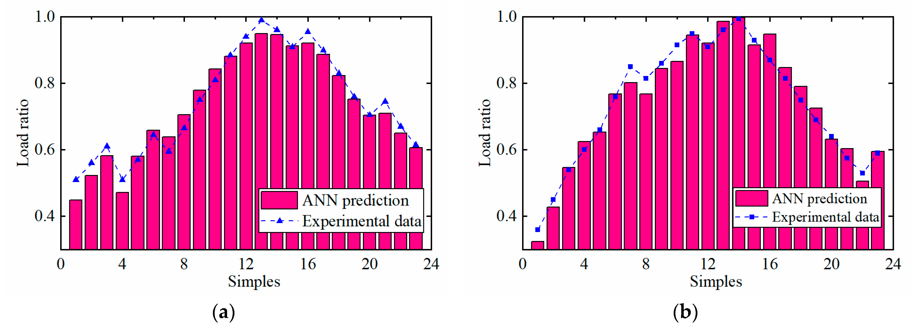
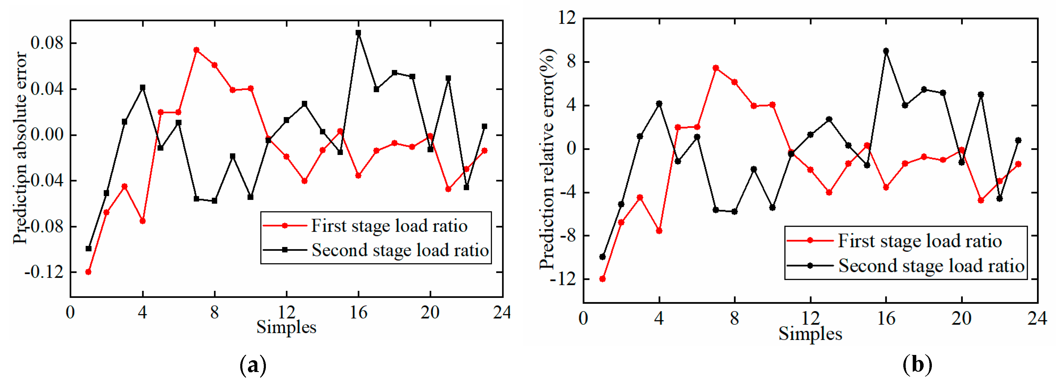
Figure 18 displays the comparison of the test results of the conventional ANN model and the experimental data. It can be seen that the overall prediction trend is acceptable. To further evaluate the conventional ANN model, prediction errors are shown in Figure 19. It can be concluded that the ANN model had high prediction errors at some points. As can be seen in Figure 19a, the maximum prediction absolute error of the first-stage load ratio reached up to −0.12, and the maximum prediction absolute error of the second-stage load ratio was −0.1. Most of their absolute prediction errors were between −0.05 and 0.05. Figure 19b indicates the relative prediction errors. It can be observed that their relative prediction errors were in the range of −12% to 8%.

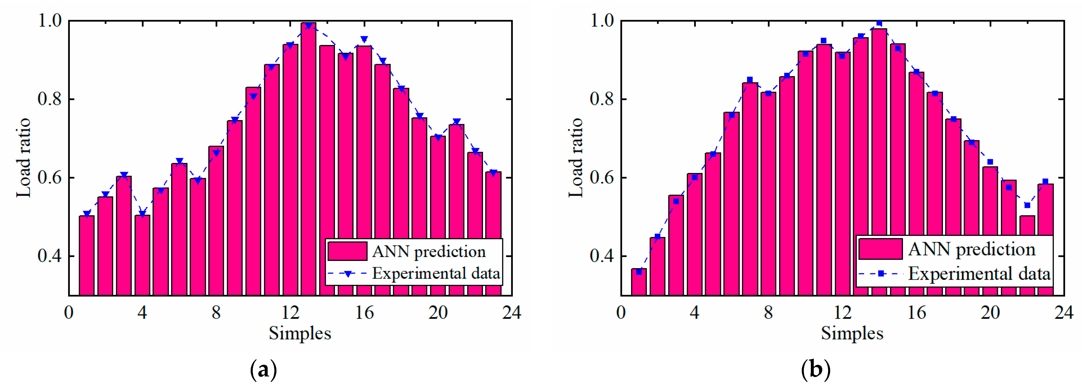
To improve the prediction precision, particle swarm optimization is used to optimize the initial weight and threshold of the ANN model. Figure 20 shows a comparison of ANN test results with PSO and experimental data. Compared with Figure 18, ANN predictions with PSO matched better with the experimental data. Therefore, it can be concluded from Figure 18 and Figure 20 that the ANN model established in this work shows great robustness no matter whether PSO is adopted or not. 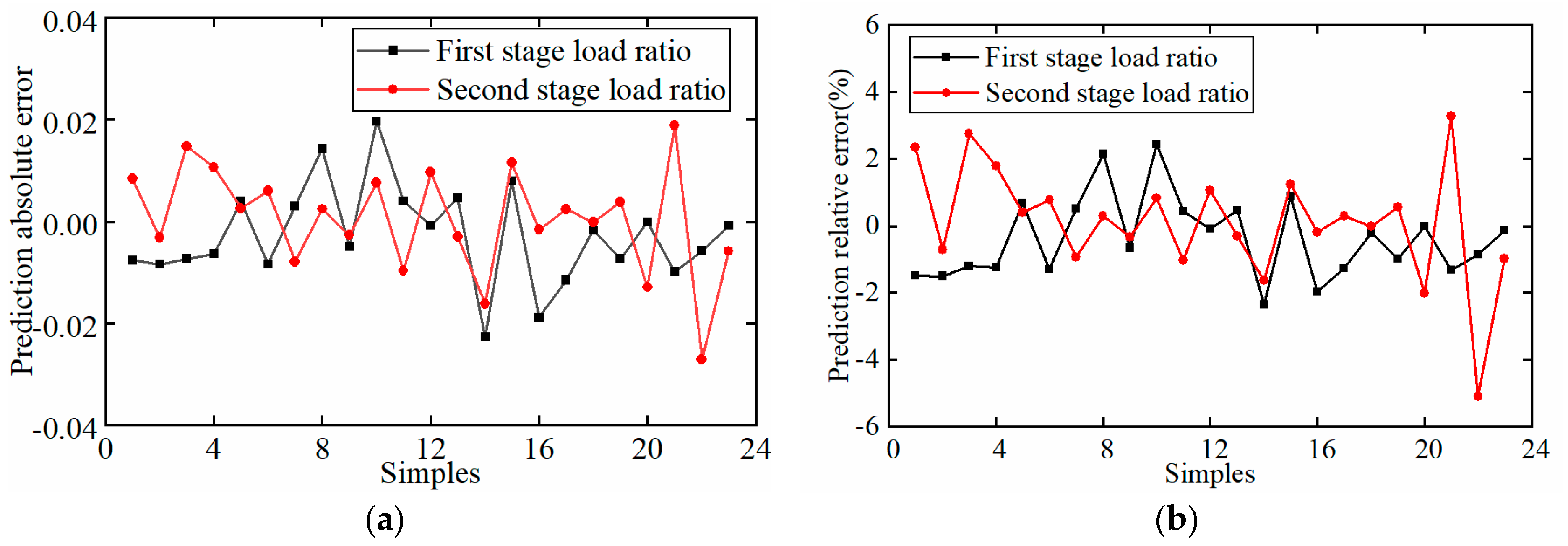Figure 21 displays the prediction errors of the ANN model with PSO. It can be seen that the prediction errors of the ANN model with PSO were lower than without PSO, as shown in Figure 21. Most of the absolute prediction errors of the ANN model with PSO were between −0.02 and 0.02, while the relative prediction errors ranged from −2% to 2%. Compared with the experimental data, the maximum relative error was less than 4%. Therefore, the proposed ANN model with PSO shows strong learning ability and good generalization performance and can be used to predict the power output of the capacity regulation system.

To verify the consistency of the optimization results, the conventional ANN model and the modified ANN model with PSO were trained repeatedly (five times). After each training, the test data were tested, and it was found that in different tests, the prediction deviation of the traditional ANN model was larger at some points, while the improved ANN model was close to the real value every time. Therefore, the optimization results show a good consistency.

5.3. Parametric Optimization Based on ANN Model

It is explained in Section 3 that the capacity regulation system realizes the capacity regulation of the compressor by controlling the energizing time of the high-speed solenoid valve. The calculation formulas of the energizing time of solenoid valve are Equations (10) and (11). In order to facilitate the compensation optimization of control parameters, Equations (10) and (11) are converted into the following forms.

$$\begin{array}{c}{T}_{control}=T_{c0}+f\left(\eta \right)\\ T_{c0}=\frac{60}{n}-t_0-t_{off}\end{array}$$

(19)

where $T_{control}$ represents the output control signal, that is, the solenoid valve total energizing time, T₀, representing the shortest energized time of the solenoid valve, is determined by the initial response characteristic of the solenoid valve and the designed stiffness of the actuator spring and the phase of the actuator to complete the ejection action. f (η) is the relationship between the load and the increase in energized time and can be expressed as:

$$f\left(\eta \right)=\frac{1}{\omega }\{\arccos \left(\frac{1}{\lambda }-\sqrt{1+\frac{2}{\lambda }-\frac{4\eta }{\lambda }+\frac{1}{{\lambda }^2}}\right).$$

(20)

In order to realize system regulation optimization, the optimization compensation item is introduced into Equation (19) to overcome system regulation degradation caused by spring stiffness degradation or (and) changes in the dynamic characteristics of the electro-hydraulic actuator.

$$T_{control}=T_{c0}+f\left(\eta \right)+\Delta T_c.$$

(21)

To obtain the system optimization compensation parameter $\Delta T_c$ and to evaluate the degradation efficiency of the capacity regulation system, the deviation of the load was taken into account. To simplify the optimization objective, we computed the degradation rate of the SCRS as follows:

$$E=\frac{100\sqrt{{{\displaystyle \sum _{i=1}^m\left({\tilde{\eta }}_i-{\eta }_i\right)}}^2}}{m},$$

(22)

where ${\tilde{\eta }}_i$ is the load feedback value which can be calculated by the ANN prediction model, ${\eta }_i$ is the given load output to the actuator, and m is the number of compressor stages. The optimization objective is the minimized degradation rate E in (22). Since the optimization is a steady-state optimization, an adaptive optimization method based on the degradation rate of SCRS is proposed to reduce the over-optimization caused by the load prediction error. If the degradation rate is low, the compensation amount of the control signal is small, ensuring no over-optimization. On the contrary, when the degradation rate is high, a large amount of compensation is generated to accelerate the system performance recovery. Therefore, the following adaptive adjustment formula can be used to optimize control signal compensation.

$$\Delta T_{ci}=\frac{2}{\pi }arctan\left({\alpha }_{i}E\right)\left[f\left({\eta }_i\right)-f\left({\tilde{\eta }}_i\right)\right],$$

(23)

where ${\alpha }_i$ is a constant that influences the speed of parameter optimization, and E is the degradation rate. The parameter ${\alpha }_i$ can be adjusted according to the performance of the system optimization.

5.4. The Implementation Effect of the Optimization Method

In order to verify the proposed system parameter optimization method, two experimental tests were carried out on a two-stage reciprocating compressor test bench equipped with SCRS as shown in Figure 3.

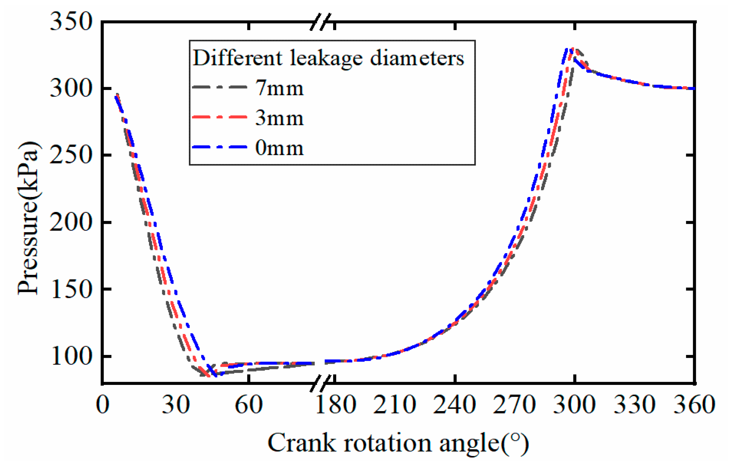
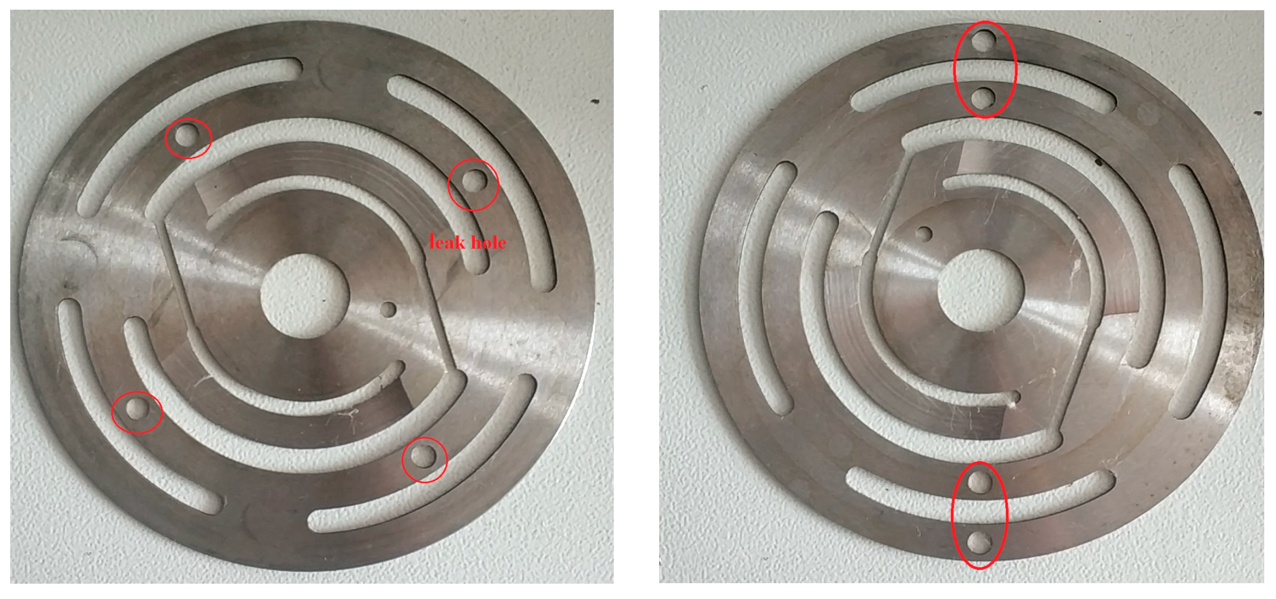
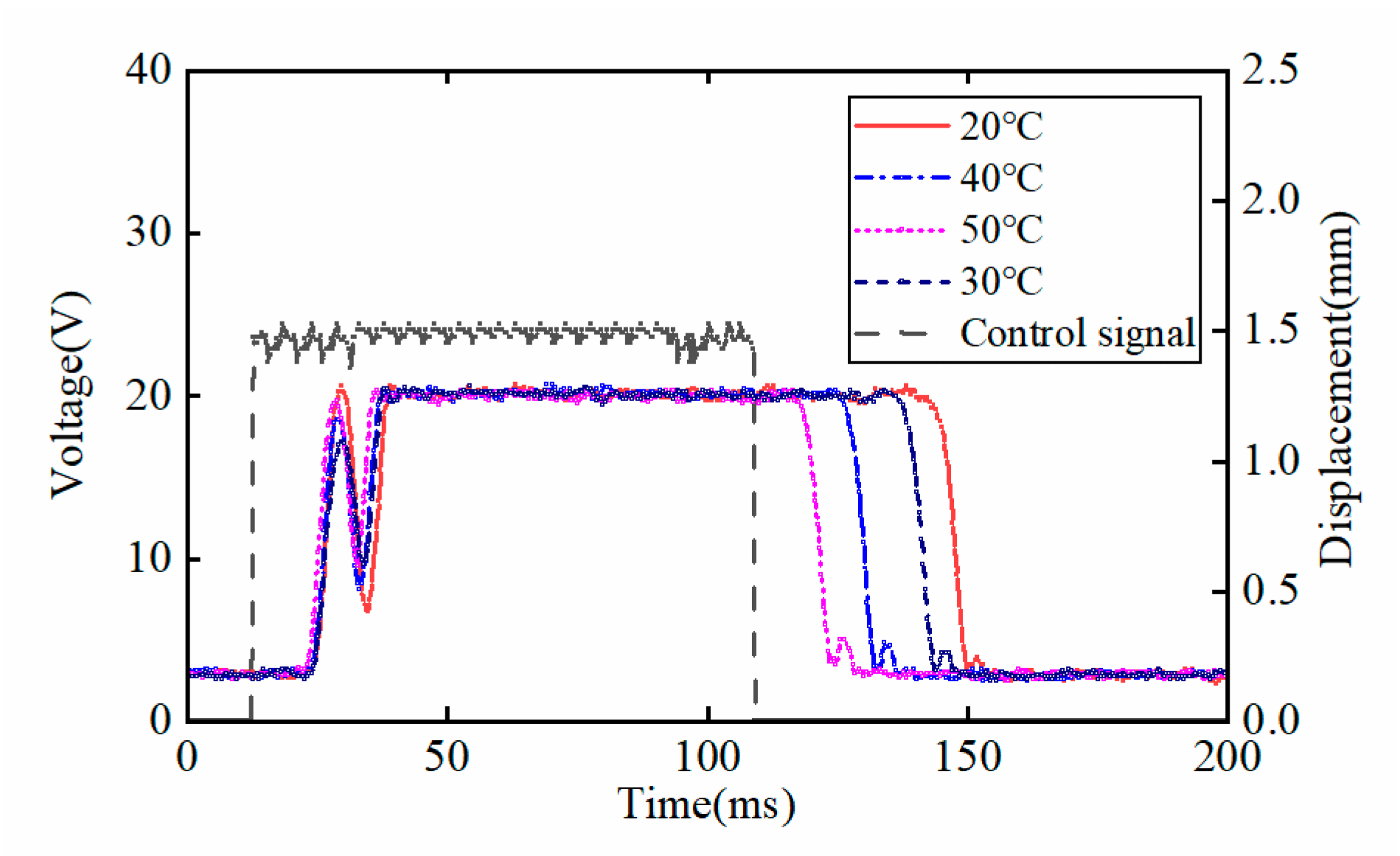
In order to accurately know the delayed closing phase of the valve plate, a displacement sensor was installed inside the actuator to test the real-time displacement of the valve plate which is extremely dangerous in practical applications and is not allowed. Figure 22 shows the simulation of valve leakage by making leak holes into the suction valve plate. The comparison of the actuator response tested by the displacement sensor at different hydraulic oil temperatures is shown in Figure 23. It was found that under the same control signal, the actuator’s response became faster as the temperature of the hydraulic oil increased. Therefore, it is possible to change the temperature of the hydraulic oil to replace the change in solenoid valve performance and spring stiffness to affect the system regulation performance.

Under the normal condition of the SCRS, the given load of the first and the second stage are both 80%. After the capacity regulation was stable, the operating condition of the SCRS was changed. The normal operation condition of the SCRS is that all valves have no leakage and the temperature of the hydraulic oil is 35 °C. The effectiveness of the optimization method was proved by the following two test experiments.

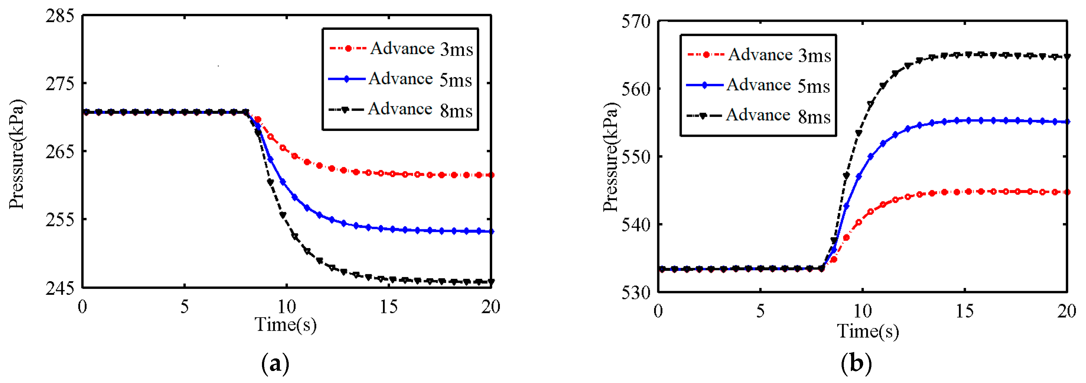
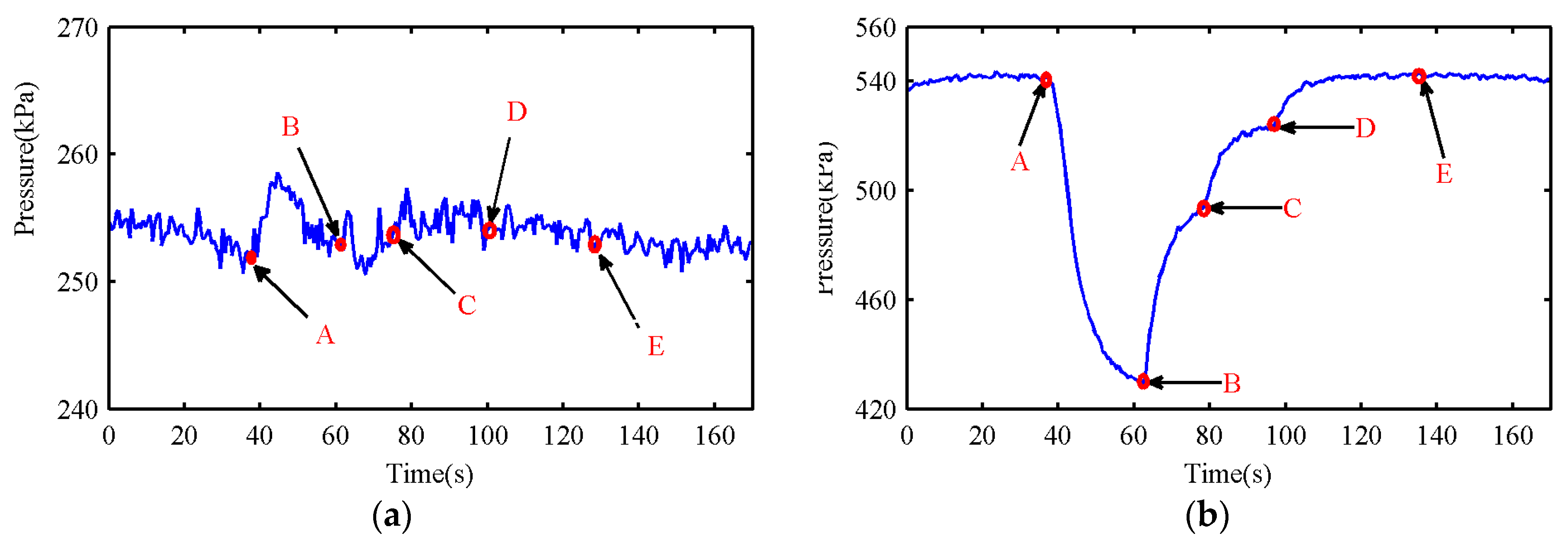
Experiment 1.

Valve leaks in the first stage caused the hydraulic temperature driving the high-pressure stage actuator to rapidly drop from 35 to 25 °C. The optimization result was adjusted by adjusting the adaptive optimization parameter. In this study, the parameter was set as α = [0.6, 0.6].

Figure 24 shows that the system was in normal operation until point A, and the pressure of the first and the second exhaust buffer tank were stable at 251 kPa and 541 kPa, respectively. Leakage holes were made in the first-stage suction valve between point A and point B, and at the same time the second-stage hydraulic oil was rapidly cooled from 35 to 25 °C. When the steady-state point B was reached, the system optimization function started to work, and the adaptive control parameter compensations were generated. Similarly, the optimized compensations were generated at the stable point C and point D, respectively. The compensation amount and predicted load at different points are shown in

Table 6. Implementation optimization results of Experiment 1.

Curve Position	Pressure (kPa)	Temperature (°C)	Prediction Load (%)	Load Deviation	Degradation Rate E	Parameter Compensation (ms)
A	251/541	33/33	77.5/83.2	2.5/−3.2	2.03	−0.6/1.56
B	252/429.7	33/33	64.8/60.7	15.2/19.3	12.28	−10/−12.1
C	254/494	33/34	72.7/72.3	7.3/7.7	5.31	−5/−4.9
D	254/524	33/34	76.1/78.3	3.9/2.7	2.32	−1.3/−0.67
E	252/542	33/35	78/82	2/−2	1.41	−0.5/1.24

. Since the compensation amount was generated adaptively according to the degradation rate of the system, the compensation amount decreased with the decrease of the degradation rate. At point B, the system degradation rate was 12.28. With the help of optimization, the system degradation rate eventually decreased to 1.41, which is very close to 2.03 under normal conditions. The deviation between the final pressure at the optimized completion point E and the pressure under normal working conditions was 1 kPa. The adaptive optimization strategy ensured that there was no over-optimization in the case of errors in the load prediction, and the duration of the whole optimization was 50 s.

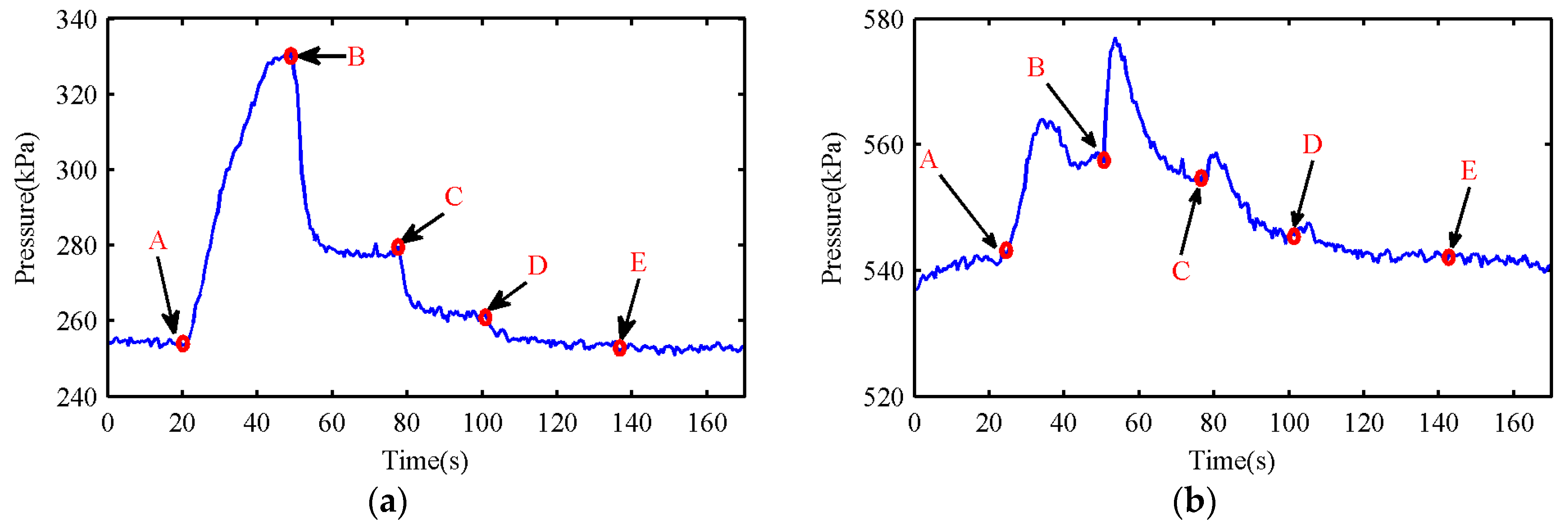
Experiment 2.

The temperature of the hydraulic oil driving the low-pressure stage actuator increased rapidly from 35 to 45 °C, while the temperature of the hydraulic oil driving the high-pressure stage actuator decreased rapidly from 35 to 25 °C.

The temperature of the hydraulic oil was 35 °C under normal working conditions. The given load of the first and the second stage were both 80%, and the pressure in the steady state was 253 kPa and 543 kPa, respectively. The temperature of the hydraulic oil driving the first actuator was raised from 35 to 45 °C, and the temperature of the hydraulic oil driving the second actuator was lowered from 35 to 25 °C. Figure 25 shows that the pressure of the first exhaust buffer tank rose rapidly, and the pressure of the second exhaust buffer tank rose slightly. When it reached the stable point B, the system started to optimize to overcome the load deviation caused by the change of hydraulic temperature. After repeated optimization, the pressure of the first-stage exhaust buffer tank decreased from 331 to 252 kPa and returned to the normal range. The results of multiple optimizations are shown in

Table 7. Implementation optimization results of Experiment 2.

Curve Position	Pressure (kPa)	Temperature (°C)	Prediction Load (%)	Load Deviation	Degradation Rate E	Parameter Compensation (ms)
A	253/541	33/35	78.2/82.1	2/−2	1.41	−0.5/1.2
B	331/557	33/36	92/56.2	−12/24.8	13.78	11.7/−14
C	279/554	33/36	88.2/73.8	−8.2/6.2	5.14	6.3/−4
D	261/546	33/36	83/82	−3/−2	1.80	1.45/1.45
E	252/542	33/36	78.5/82.6	1.5/−2.6	1.50	−0.51/1.29

. After optimizing twice, the degradation rate of the system decreased from the maximum 13.78 to 1.8, and the duration of the whole optimization was 60 s.

6. Conclusions

Aiming to overcome the performance degradation and the regulation accuracy decrease of SCRS for reciprocating compressors in long-term running processes, in this paper, the mathematical model of multi-subsystem coupling was established to analyze the key components and parameters that affect the regulating performance of the system, such as dynamic characteristics of the solenoid valve, reset spring stiffness, and valve leakage. The law of system performance degradation was obtained.

In order to restore the regulation performance and precision of the system when the system degenerates, firstly, the PSO-BP load prediction model was established, and the model was trained and tested with experimental data. The results show that the load prediction error of the improved PSO-BP model was less than 2%. The actual load of the compressor was predicted online by using steady state pressure, temperature, and flow rate, and the system degradation rate was calculated. A system control parameters compensation optimization method based on predictive load and system degradation rate was proposed. Secondly, in order to prevent overcompensation of the control parameters, an adaptive optimization compensation method was developed, and the compensation amount of the control parameters was adjusted adaptively according to the degradation rate. Finally, two system optimization experiments were set up, and the experimental results verified the feasibility and effectiveness of the compensation optimization method in this paper.

Therefore, the system compensation optimization framework proposed in this paper provides an effective solution to the field performance degradation of the stepless capacity regulating system for reciprocating compressors. However, this framework can be expanded to any other complex mechatronics system.

References

1. Li, D.; Wu, H.; Gao, J. Experimental study on stepless capacity regulation for reciprocating compressor based on novel rotary control valve. Int. J. Refrig. 2013, 36, 1701–1715. [Google Scholar] [CrossRef]
2. Richard, B. Infinitely Variable Capacity Control System for Compressors and Device for Stepless Regulating According to this System. US Patent 3,255,955, 14 June 1966. [Google Scholar]
3. Hong, W.; Jin, J.; Wu, R. Theoretical analysis and realization of stepless capacity regulation for reciprocating compressors. Proc. Inst. Mech. Eng. Part E J. Process Mech. Eng. 1996, 223, 205–213. [Google Scholar] [CrossRef]
4. Jin, J.; Hong, W. Valve dynamic and thermal cycle model in stepless capacity regulation for reciprocating compressor. Chin. J. Mech. Eng. 2012, 25, 1151–1160. [Google Scholar] [CrossRef]
5. Tang, B. Dynamic Analysis of Valve with Stepless Capacity Control for Reciprocating Compressor. J. Mech. Eng. 2011, 47, 136–141. [Google Scholar] [CrossRef]
6. Tang, B.; Zhao, Y.; Li, L. Thermal performance analysis of reciprocating compressor with stepless capacity control system. Appl. Therm. Eng. 2013, 54, 380–386. [Google Scholar]
7. Tang, B.; Zhao, Y.; Li, L. Dynamic characteristics of suction valves for reciprocating compressor with stepless capacity control system. Proc. Inst. Mech. Eng. Part E J. Process Mech. Eng. 2014, 228, 104–114. [Google Scholar] [CrossRef]
8. Zhao, Y.; Tang, B.; Liu, G. Experimental research on dynamic response of capacity system in reciprocating compressor. Proc. Inst. Mech. Eng. Part C J. Mech. Eng. Sci. 2014, 228, 358–365. [Google Scholar]
9. Li, Y.; Xuan, H.J.; Hong, W.R. Analysis of rod reversal in reciprocating compressor with capacity regulating system. J. Process Mech. Eng. 2017, 231, 131–137. [Google Scholar] [CrossRef]
10. Wang, Y.; Jiang, Z.N.; Zhang, J.J.; Zhou, C. Performance analysis and optimization of reciprocating Compressor with stepless capacity control system under variable load conditions. Int. J. Refrig. 2018, 94, 174–185. [Google Scholar] [CrossRef]
11. Liu, G.B.; Zhao, Y.Y.; Tang, B. Dynamic performance of suction valve in stepless capacity regulation system for large-scale reciprocating compressor. Appl. Therm. Eng. 2016, 96, 167–177. [Google Scholar] [CrossRef]
12. Liu, G.B.; Tang, B. Dynamic Performance of Reciprocating Compressor with Capacity Stepless Regulation System. J. Mech. Eng. 2017, 53, 26–31. [Google Scholar] [CrossRef]
13. Belman-Flores, J.M.; Ledesma, S. A comparison between the modeling of a reciprocating compressor using artificial neural network and physical model. Int. J. Refrig. 2015, 59, 144–156. [Google Scholar] [CrossRef]
14. Barroso-Maldonado, J.M.; Belman-Flores, J.M.; Ledesma, S.; Rangel-Hernández, V.H.; Cabal-Yépez, E. Predicting the energy performance of a reciprocating compressor using artificial neural networks and probabilistic neural networks. Rev. Mex. De Ing. Quim. 2017, 16, 679–690. [Google Scholar]
15. Kim, D.W.; Song, K.S.; Lim, J.; Kim, Y. Analysis of two-phase injection heat pump using artificial neural network considering APF and LCCP under various weather conditions. Energy 2018, 155, 117–127. [Google Scholar] [CrossRef]
16. Singh, S.; Dasgupta, M.S. Performance evaluation of a CO2 scroll expander for work recovery using artificial neural network. Sci. Technol. Built Environ. 2018, 24, 580–587. [Google Scholar] [CrossRef]
17. Mohammadi, M.; Lakestani, M.; Mohamed, M.H. Intelligent parameter optimization of Savonius rotor using Artificial Neural Network and Genetic Algorithm. Energy 2018, 143, 56–68. [Google Scholar] [CrossRef]
18. Bensingh, R.J.; Machavaram, R.; Boopathy, S.R.; Jebaraj, C. Injection molding process optimization of a bi-aspheric lens using hybrid artificial neural networks (ANNs) and particle swarm optimization (PSO). Measurement 2019, 134, 359–374. [Google Scholar] [CrossRef]
19. Yang, F.B.; Cho, H.; Zhang, H.G. Artificial neural network (ANN) based prediction and optimization of an organic Rankine cycle (ORC) for diesel engine waste heat recovery. Energy Convers. Manag. 2018, 164, 15–26. [Google Scholar] [CrossRef]
20. Elhaj, M.; Gu, F.; Ball, A.D. Numerical simulation and experimental study of a two-stage reciprocating compressor for condition monitoring. Mech. Syst. Signal Process. 2008, 22, 374–389. [Google Scholar] [CrossRef]
21. Richer, E.; Hurmuzlu, Y. A High Performance Pneumatic Force Actuator System: Part I—Nonlinear Mathematical Model. J. Dyn. Syst. Meas. Control 2000, 122, 416–425. [Google Scholar] [CrossRef]
22. Zhang, B.; Zhong, Q. Self-correcting PWM control for dynamic performance preservation in high speed on/off valve. Mechatronics 2018, 55, 141–150. [Google Scholar] [CrossRef]
23. Zhang, C.W. Control Force Characteristics of Different Control Strategies for the Wind-Excited 76-Story Benchmark Building Structure. Adv. Struct. Eng. 2014, 17, 543–559. [Google Scholar] [CrossRef]
24. Wu, J.; Li, Z.; Zhu, L.; Li, G.Y. Optimized BP neural network for dissolved oxygen prediction. IFAC Pap. 2018, 51, 596–601. [Google Scholar] [CrossRef]
Figure 1. Proposed framework for compensation optimization.
Applsci 10 00704 g001
Figure 2. The variable capacity reciprocating compressor pressure system.
Applsci 10 00704 g002
Figure 3. Two-stage reciprocating compressor with a stepless capacity regulation system (SCRS).
Applsci 10 00704 g003
Figure 4. Simplified physical model of gas pipeline.
Applsci 10 00704 g004
Figure 5. Dynamic pressure in the cylinder under different loads.
Applsci 10 00704 g005
Figure 6. Simulation and experimental data of buffer tank pressure; (a) the first stage; (b) the second stage.
Applsci 10 00704 g006
Figure 7. Control signal, suction valve plate, unloader, and cylinder dynamic pressure.
Applsci 10 00704 g007
Figure 8. Dynamic process under different control signals.
Applsci 10 00704 g008
Figure 9. Valve plate, actuator displacement, and cylinder pressure under different spring stiffness values.
Applsci 10 00704 g009
Figure 10. (a) First-stage exhaust buffer tank pressure; (b) second-stage exhaust buffer tank pressure.
Applsci 10 00704 g010
Figure 11. Solenoid valve response, valve plate displacement, and dynamic pressure.
Applsci 10 00704 g011
Figure 12. (a) First-stage exhaust buffer tank; (b) second-stage exhaust buffer tank.
Applsci 10 00704 g012
Figure 13. The cylinder pressure with different diameter leakage hole under full load condition.
Applsci 10 00704 g013
Figure 14. The cylinder pressure with different leakage diameter holes under the regulating condition.
Applsci 10 00704 g014
Figure 15. Area ratio of p-v diagram under different leakage diameters.
Applsci 10 00704 g015
Figure 16. Prediction model structure diagram. (a) three-layer artificial neural network model; (b) the training process.
Applsci 10 00704 g016
Figure 17. The calculation procedure of particle swarm optimization back propagation (PSO-BP) method.
Applsci 10 00704 g017
Figure 18. Comparison of conventional artificial neural network (ANN) predictions and experimental data; (a) the first stage; (b) the second stage.
Applsci 10 00704 g018
Figure 19. (a) Prediction absolute error of conventional ANN model; (b) relative prediction error of conventional ANN model.
Applsci 10 00704 g019
Figure 20. Comparison of modified ANN predictions and experimental data with PSO; (a) the first stage; (b) the second stage.
Applsci 10 00704 g020
Figure 21. (a) Absolute prediction error of the ANN model with PSO; (b) relative prediction error of the ANN model with PSO.
Applsci 10 00704 g021
Figure 22. Suction valve plate leakage hole.
Applsci 10 00704 g022
Figure 23. Solenoid valve response curve at different temperatures.
Applsci 10 00704 g023
Figure 24. (a) First-stage exhaust buffer tank pressure of Experiment 1; (b) second-stage exhaust buffer tank pressure of Experiment 1.
Applsci 10 00704 g024
Figure 25. (a) First-stage exhaust buffer tank pressure of Experiment 2; (b) second-stage exhaust buffer tank pressure of Experiment 2.
Applsci 10 00704 g025