Stochastic Recognition of Physical Activity and Healthcare Using Tri-Axial Inertial Wearable Sensors


1
Department of Computer Science, Air University, Islamabad 44000, Pakistan
2
Department of Human-Computer Interaction, Hanyang University, Ansan 15588, Korea
*
Author to whom correspondence should be addressed.
Appl. Sci. 2020, 10(20), 7122; https://0-doi-org.brum.beds.ac.uk/10.3390/app10207122
Submission received: 11 August 2020
/
Revised: 18 September 2020
/
Accepted: 10 October 2020
/
Published: 13 October 2020
(This article belongs to the Section Electrical, Electronics and Communications Engineering)
Abstract
:Featured Application
The proposed technique is an application of physical activity detection, analyzing three challenging benchmark datasets. It can be applied in sports assistance systems that help physical trainers to conduct exercises, track functional movements, and to maximize the performance of people. Furthermore, it can be applied in surveillance system for abnormal events and action detection.
Abstract
The classification of human activity is becoming one of the most important areas of human health monitoring and physical fitness. With the use of physical activity recognition applications, people suffering from various diseases can be efficiently monitored and medical treatment can be administered in a timely fashion. These applications could improve remote services for health care monitoring and delivery. However, the fixed health monitoring devices provided in hospitals limits the subjects’ movement. In particular, our work reports on wearable sensors that provide remote monitoring that periodically checks human health through different postures and activities to give people timely and effective treatment. In this paper, we propose a novel human activity recognition (HAR) system with multiple combined features to monitor human physical movements from continuous sequences via tri-axial inertial sensors. The proposed HAR system filters 1D signals using a notch filter that examines the lower/upper cutoff frequencies to calculate the optimal wearable sensor data. Then, it calculates multiple combined features, i.e., statistical features, Mel Frequency Cepstral Coefficients, and Gaussian Mixture Model features. For the classification and recognition engine, a Decision Tree classifier optimized by the Binary Grey Wolf Optimization algorithm is proposed. The proposed system is applied and tested on three challenging benchmark datasets to assess the feasibility of the model. The experimental results show that our proposed system attained an exceptional level of performance compared to conventional solutions. We achieved accuracy rates of 88.25%, 93.95%, and 96.83% over MOTIONSENSE, MHEALTH, and the proposed self-annotated IM-AccGyro human-machine dataset, respectively.
1. Introduction
Chronic and physical fitness-related diseases are rapidly increasing as the population increases. Physical activities are directly associated with human health benefits. Therefore, many researchers strongly recommend 30 to 40 minutes of physical activity regularly for a healthier life, since it can reduce the risk of many diseases, such as heart attacks, diabetes, cancer, cardiovascular disease, and so on [1]. In hospitals, many patients need continuous monitoring, which is quite expensive and inconvenient, especially for children and elderly people [2]. Instead of relying on expensive treatments and delayed intervention, healthcare sensing technology can inform doctors of escalated incidents beforehand. Among the primary health-care sensing categories, wearable inertial sensors show promising potential for human locomotion tracking [3]. These sensors can monitor human activities conveniently and effectively in a free living environment, and their use is rapidly increasing, representing up to 97% of the market volume by 2020 [4].
Human activity recognition (HAR) can be broadly classified into template matching, generative and discriminative categories [5,6]. Firstly, template matching algorithms, such as the K-Nearest Neighbors classifier, compute the distances between the event data. Secondly, generative algorithms, e.g., the Bayes network, use probabilistic graphs to classify human activities. Finally, discriminative approaches model the boundaries between data events [7,8,9]. Although these machine learning algorithms operate with little prior information, they nevertheless provide good classification results [10,11,12,13,14,15]. However, their feature engineering requires deep expertise that can significantly reduce discriminant errors and improve the performance of a recognition system.
In this paper, we propose new robust ‘multi-combined’ features to represent human body movements and to classify human activity patterns using the time-series data from tri-axial inertial signals via wearable sensors. These new features are combinations of 14 different kinds of features, including statistical features, the Mel Frequency Cepstral Coefficients (MFCC), Electrocardiogram (ECG) features, and Gaussian Mixture Model (GMM) features, which efficiently reduce discriminant errors and improve the performance of the activity recognition system. For HAR, novel combined classifiers such as Binary Grey Wolf Optimization (BGWO) and Decision Trees (DTs) are applied. To examine the performance, a new continuous wearable human activity dataset (i.e., the IM-AccGyro dataset) that contains 1D segmented signal sequences is provided; this can be used for the training and testing data of different physical exercises. This will become a benchmark dataset in the field of the wearable activity recognition of physical exercises based on inertial sensors. Additionally, we apply the proposed method to public datasets such as the MOTIONSENSE and MHEALTH datasets. For comparison studies, we consider state-of-the-art methods such as a Genetic algorithm optimized by Ant Colony Optimization (ACO) and a Support Vector Machine (SVM) optimized by Particle Swarm Optimization (PSO). We obtained remarkable improvements in the recognition rates over current state-of-the-art methods.
The rest of this paper is organized as follows. Section 2 presents related works. Section 3 presents the complete system methodology, which is comprised of physical activity detection, preprocessing, feature extraction, optimization, and classification methodologies. Section 4 explains the complete experimental setting and describes the datasets. Section 5 describes the results and evaluation. Finally, Section 6 presents the conclusion.
2. Related Works
Several studies have classified human activity patterns. These activity patterns have been classified using two major categories of sensor devices: vision sensors and wearable sensors. In vision-based HAR, video cameras are used to capture image data. Babiker et al. [16] proposed digital image processing techniques including background subtraction, binarization, and morphological operations. Then, a multilayer feed-forward perceptron network is applied to recognize daily human movements and to conduct HAR in indoor environments with a single static camera. Jalal et al. [17] obtained video-based invariant features by applying the R transform to depth silhouettes. These silhouettes are encoded into feature values using depth images. Then, the scaling invariant features are calculated by computing the 2D and 1D features using Radon transform and R transform. Finally, principal component analysis and the Hidden Markov Model are applied to the computed features to train and recognize different human activities. Liu et al. [18] focused on the shapelet-based method to recognize four different types of human activities. They evaluated their proposed approach on two public datasets. Experimental results showed their proposed approach was efficient to handle complex activities.
Instead of relying on image data, many researchers have designed wearable sensor technologies for activity monitoring and classification. Jansi et al. [19] presented a multi-feature (time and frequency) domain to enhance the classification of eight different human activities from inertial sensors installed in smartphones. Tian et al. [20] proposed a two-layer diversity-enhanced multi-classifier recognition method from one triaxle accelerometer to classify four different activities. Furthermore, they extracted three-domain features (time, frequency, and AR coefficients) to optimize the performance of the multi-classifier recognition system. Tahir et al. [21] proposed a multifused model to maximize the optimal features values. The extracted features values are then optimized and classified using adaptive moment estimation and a maximum entropy Markov Model. This method achieved an accuracy of 90.91% over the MHEALTH dataset. Haresamudram et al. [22] introduced a masked reconstruction-based BERT model for human activity recognition activities. The activities are pre-trained as a self-supervised approach. The transformer encoder architecture is also applied for continuous data from body worn sensors and achieved an accuracy of 79.86% over a MOTIONSENSE dataset. Jordao et al. [23] implemented convolution neural network for wearable sensors human activity recognition data. The authors evaluated the implemented methodology on an MHEALTH dataset by using the “leave one subject out” validation protocol; they achieved an accuracy rate of 83%. Batool et al. [24] proposed a physical activity detection model based on Mel Frequency Cepstral Coefficients (MFCC) and statistical features. The extracted features were then optimized and classified with a PSO and SVM algorithm. The implemented methodology was later evaluated over a MOTIONSENSE dataset, giving an accuracy of 87.50%. Zha et al. [25] presented Logical Hidden Semi-Markov Models (LHSMMs), which are a combination of Logical Hidden Markov Models (LHMMSs) and Hidden Semi-Markov Models, to segment the duration of each activity. Moreover, a comparison of LHSMMs and LHMMs proved that the given method is more robust and has higher probability results than the LHMM method.
Optical sensors like digital and bumblebee cameras can be used to improve human lifestyles. However, there are limitations to the use of optical sensors for detecting human activities. With those sensors, the detection of subject’s movements is restricted to a particular range and they have privacy issues, e.g., recording in private places like restrooms or intruding on the user’s personal life. It is uncomfortable for the subjects to carry optical sensors around with them because sensors are bulky, invasive, and are not easily worn during working hours. Additionally, such cameras are relatively more expensive than other wearable sensors. Despite previous human activity classification research, there are still challenges in computation, multi-sensor support, and precise signal data acquisition. Therefore, we suggest a novel method for human activity classification in this paper.
3. Methodology
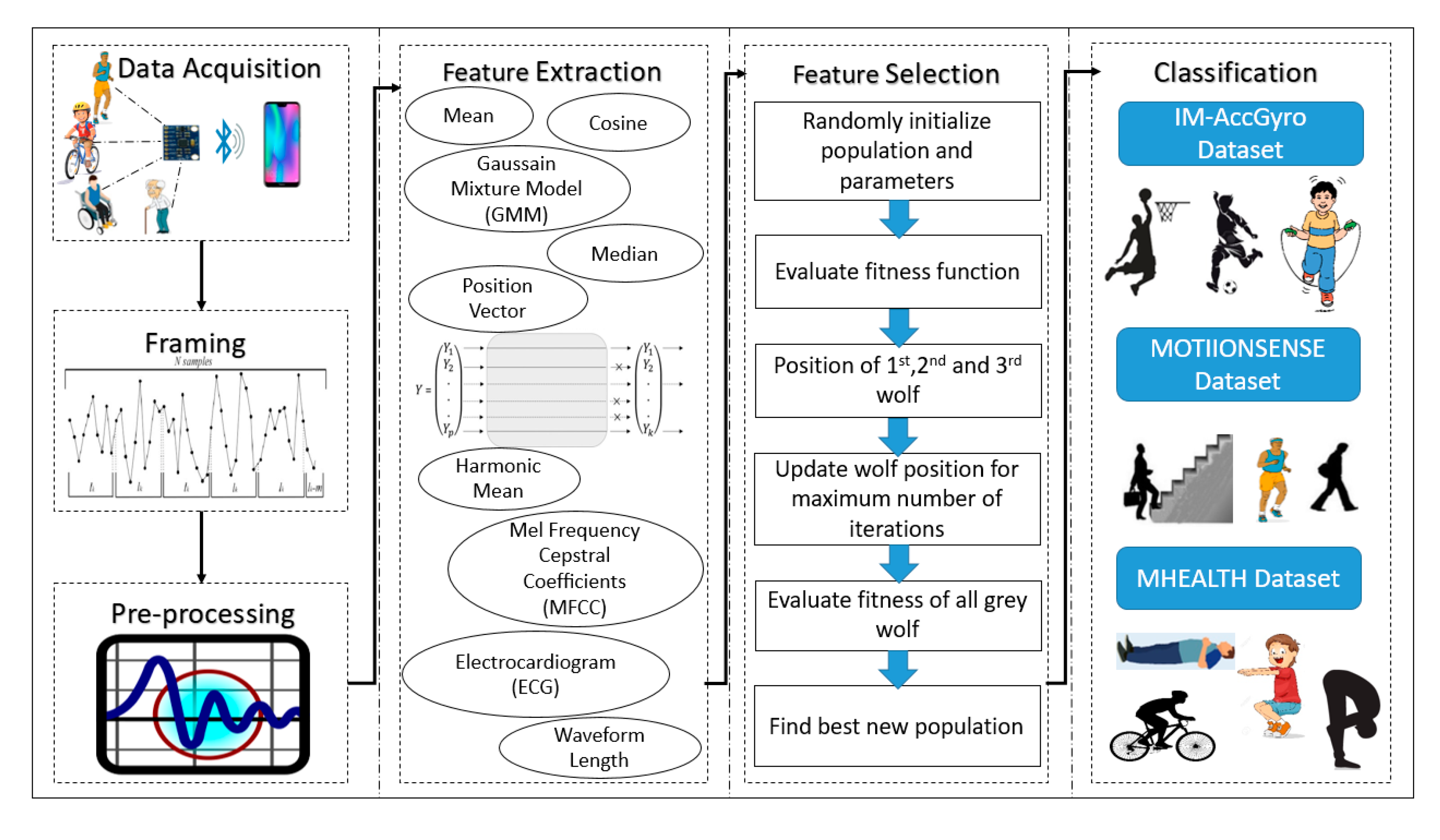
The complete framework for human activity recognition using wearable inertial sensors is depicted in Figure 1. Data are first collected by inertial sensors attached at the wrist, the knee, and the back of the participants. The collected data are preprocessed using a band-stop filter. Fourteen different features are extracted from the filtered data. Subsequently, the extracted features are optimized using BGWO. Finally, the optimized features are fed to a DT classifier to obtain the final classification. A detailed description of the system is given in the following section.
3.1. Preprocessing and Filtration of Sensor Data
Initially, signal enhancement is applied to the inertial sensor data to eliminate redundancy, irrelevancy, and inconsistency in the framed data. The band stop notch filter [26] is used for signal representation to improve the quality of data. A second-order band stop (notch) filter has two cut-off frequencies, lower cut-off and upper cut-off, which are applied to the framed data. Such a filter passes all frequencies from zero to both cutoff frequencies. All the frequencies between the lower cutoff and the upper cutoff are rejected. The bandwidth of the notch-filter is calculated by subtracting the lower cut-off frequency from the higher cut-off frequency, as shown in Figure 2. The filtered data and unfiltered data of the accelerometer signal are plotted on the same axis. The red signal represents the filtered data and the blue signal represents the unfiltered data. Moreover, an on-figure magnifier is added on the plotted accelerometer data showing the zoom-in area of the graph.
3.2. Feature Extraction and Selection
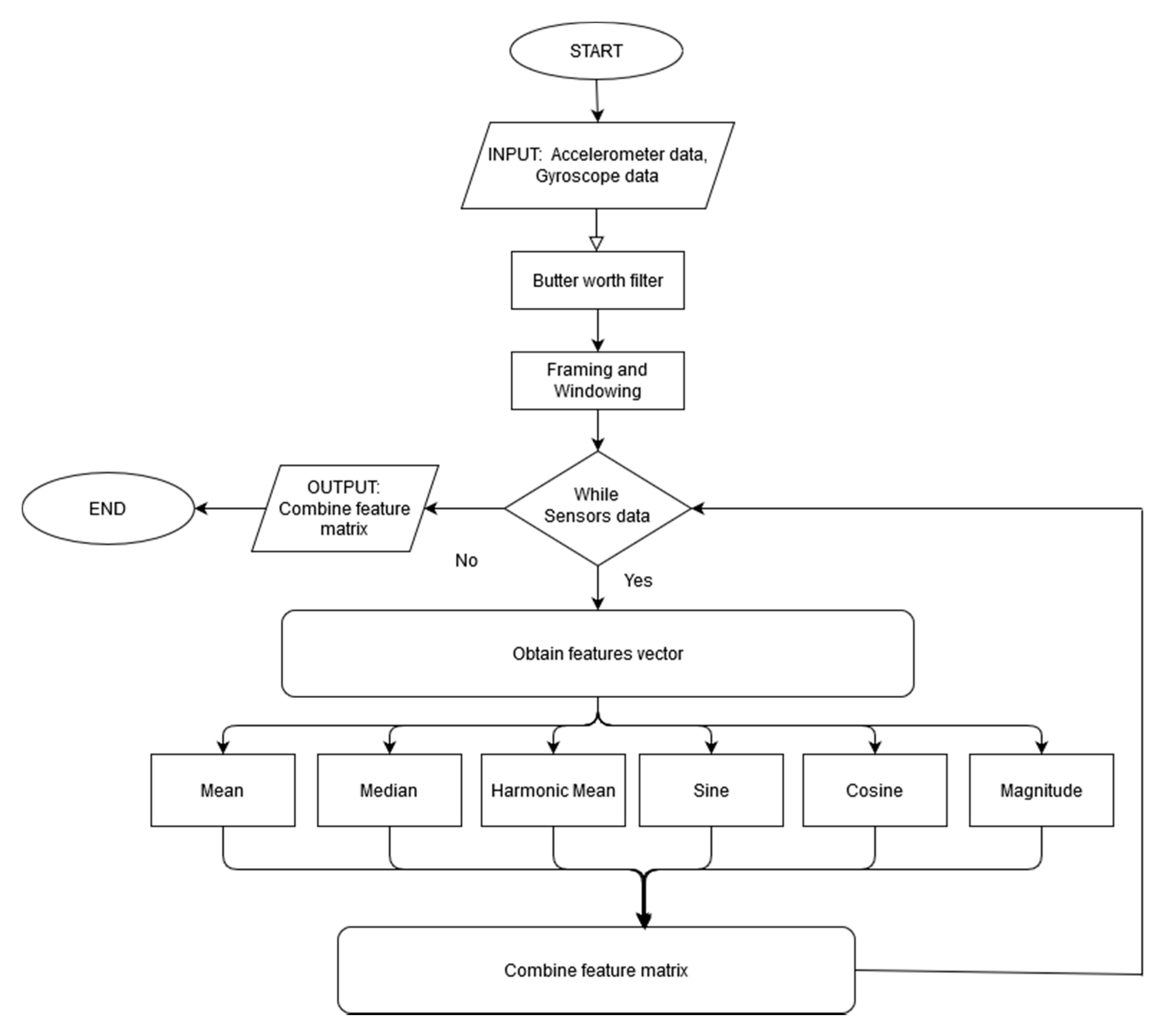
After framing and preprocessing the data, fourteen different features are extracted in each frame, including statistical features, Mel Frequency Cepstral Coefficients (MFCC) features, ECG features, and GMM features. The statistical features are computationally less intensive and can be easily extracted in real time [26,27,28]. The statistical features applied in this paper are the mean, median, harmonic mean, position vector, sine, and cosine. The MFCC features represent the frequency and amplitude of the sensor signals and are individually helpful in finding the pattern of each activity. The ECG features are commonly used to find the absolute pattern of a signal. In this paper, the ECG features include the autoregressive, waveform length, slope sign change, and Willison amplitude, which can efficiently detect the specific pattern of each activity. Furthermore, the GMM features include the weighting ratio, mean, and covariance for activity recognition. Figure 3 defines the flowchart of feature combinations as:
3.2.1. Mean Feature
The mean feature is the average value of the sampled signal in each frame [29]. It is calculated by taking the sum of the features and dividing it by the total number of samples.
3.2.2. Median Feature
The median feature is the middle value of the samples, which divides the data sample into two halves with equal numbers of observations [29]. It separates the higher half from the lower half of the sample data.
3.2.3. Harmonic Mean Feature
The harmonic mean feature HMi(t) specifically measures the reciprocal of the arithmetic mean as a ratio that gives equal weight to each data point in the sample data. It is defined as:
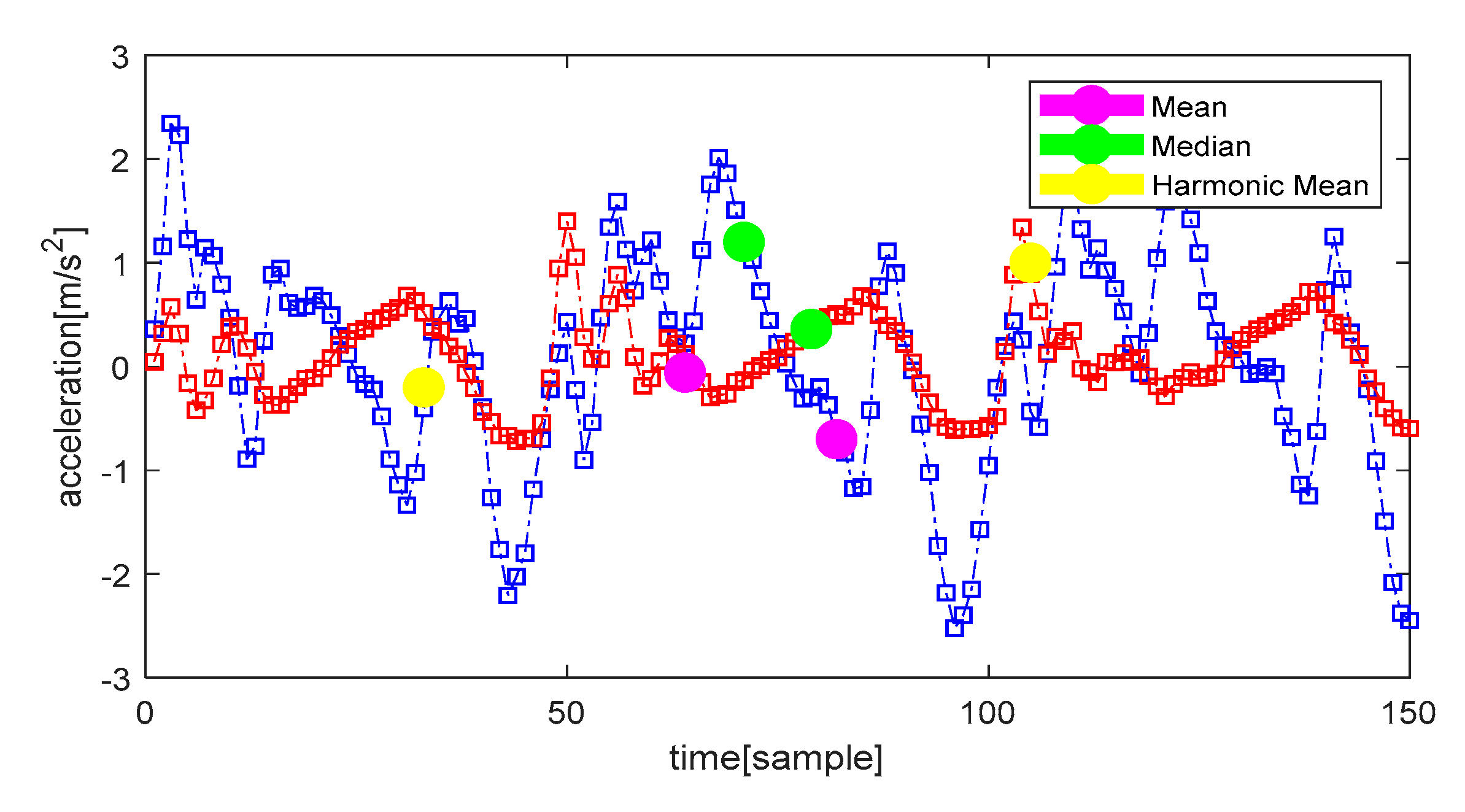
where fn is the total number of samples in each frame and fi corresponds to the current sample of the signal and ranges from fi to fi+N. Figure 4 represents the overall 1D plot of the means, medians, and harmonic means. The blue signal and red signal represent the sitting down and standing up data taken from the accelerometer. Moreover, purple dots, green dots, and yellow dots on accelerometer signals represent mean, median, and harmonic mean value, respectively.
3.2.4. Sine Feature
The sine feature SinӨ measures the angle along the x-axis by calculating the magnitude and direction angle along SinӨ. The magnitude of the sine vector measures the length of a line segment and the direction measures the angle of the ith coefficient signal values between two consecutive sample values t−1 and t. The sine magnitude and angle are defined as:
where fi and fi+1 represent the current samples of the signal, and tan−1 represents the return angle between two corresponding feature vectors fi and fi+1.
3.2.5. Cosine Feature
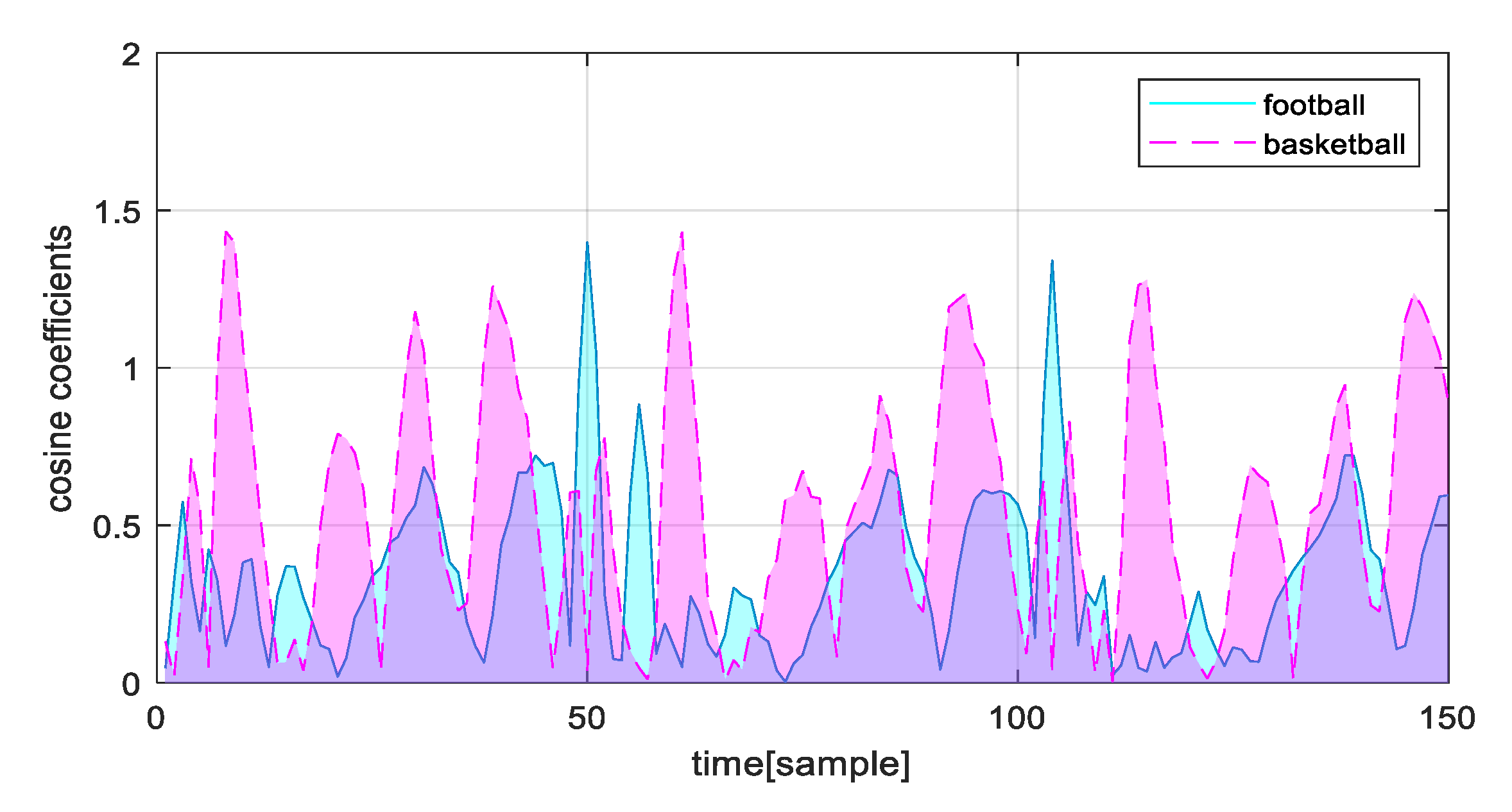
The cosine feature CosӨ measures the angle along the y-axis and calculates the magnitude and angle of a vector using the cosine feature. The magnitude of the cosine vector represents the length of a line segment from its origin to a target point (see Figure 5). Meanwhile, the direction represents the angle of the line formed along the y-axis. The cosine is defined as:
3.2.6. Position Vector Feature
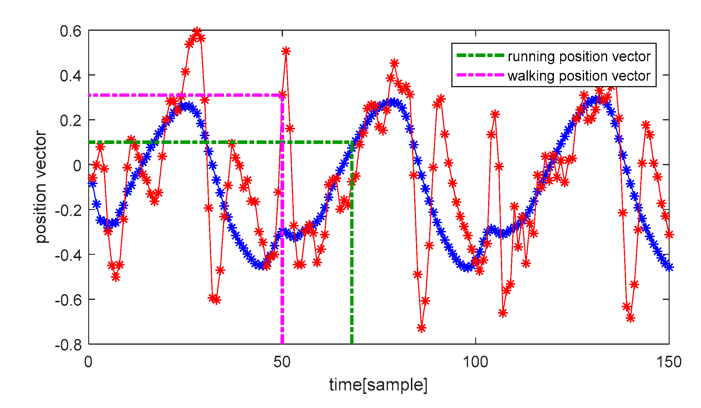
The position vector feature Pi measures the difference between the ith coefficient values between two consecutive sample values. It generates a straight line between two points and is defined as:
where fi, fi+1, and fi+2 represent the current three samples of the sensor signal, as shown in Figure 6. The running and walking activities are represented by a red signal and a blue signal. The position vector of the running activity is represented with a purple dotted line and the position vector of the walking activity is represented with a green dotted line. The purple and green dots are further extended along the x-axis and y-axis to represent them more precisely.
3.2.7. MFCC Vector Feature
The Mel Frequency Cepstral Coefficients (MFCC) measure the rate of change of information in a spectral band. These features calculate the peak values in the periodic element of a sensor signal and the resulting signal is neither in the frequency domain nor in the time domain but is in the quefrency domain. The MFCC relates the perceived signal to the actual sensor signal and is defined as:
where fn is the log filter bank amplitude, which is calculated by using a discrete cosine transform. Meanwhile, N represents the total number of filter bank channels.
3.2.8. Autoregressive Feature
The autoregressive (AR) feature samples each activity signal as a linear combination of the previous sample plus the error sequence. These features map the particular pattern of an activity and return a true value if the pattern is detected. It is specifically used for feature extraction and it is defined as:
where fn-i is the n-i feature of the sample data, ai represents the AR coefficient and the current sample of the sensor signal n is the error sequence. The second- and fourth-order ARs are used in this paper since they give the best results for each activity pattern.
3.2.9. Waveform Length Feature
The Waveform Length (WL) features are mainly used in ECG signals to measure the complexity of a signal. These are used to detect human physical activities using wearable inertial sensors. Additionally, they efficiently estimate the complexity of each activity signal by taking the negative of the current sample from the last sample and summing them. These features give the amplitude, frequency, and time information. Its formula is:
where fi is the feature vector of the current sample, fi−1 is the past sample, and N is the total number of samples in the current frame.
3.2.10. Slope Sign Change Feature
The slope sign change feature is the ratio of the vertical and horizontal changes between two sample points of a window segment. The vertical change between two sample points is called the rise, and the horizontal change is known as the run. The slope sign change is defined as:
where h and k are the x and y coordinates of a point in the signal sample in the current frame, respectively. f1 and f2 represent the current sample points.
3.2.11. Willison Amplitude Feature
The Willison amplitude is used for the detection of ECG signals. In HAR, it is defined as the number of counts for each change in the inertial sensor signal that exceeds the threshold. We used thresholds ranging from 0.01 to 0.27 to detect different human activities since they give efficient performance over time. It is defined as:
where fn and fn+1 are the current and previous samples, respectively. Meanwhile, N is the total number of samples in the current frame.
3.2.12. GMM Mean Feature
The GMM is statistically used for density estimation and clustering models. It consists of covariance matrices, a mixture weight, and a mean vector. In this paper, the GMM mean vector is calculated by using the maximum likelihood estimation that effectively estimates the mean vector of the inertial signal. It is defined as:
3.2.13. GMM Weighting Ratio Feature
The GMM weighting ratio calculates the maximum likelihood probability for the detection of each activity signal. In this paper, the GMM weighting ratio is calculated using the iterative maximization method and is defined as:
where fi is the current feature of the signal and is subtracted from the next predicted fi+1 feature of the signal to estimate the weighted ratio of the current feature.
3.2.14. GMM-Based Covariance Ratio Feature
The GMM covariance measures the joint variability of two samples in the current window. The result of the covariance is always positive for a greater value of the second data sample and vice versa.
where µx is the mean of the current sample fi, and µy is the mean of the previous sample fi−1.
3.3. Basic Classifier
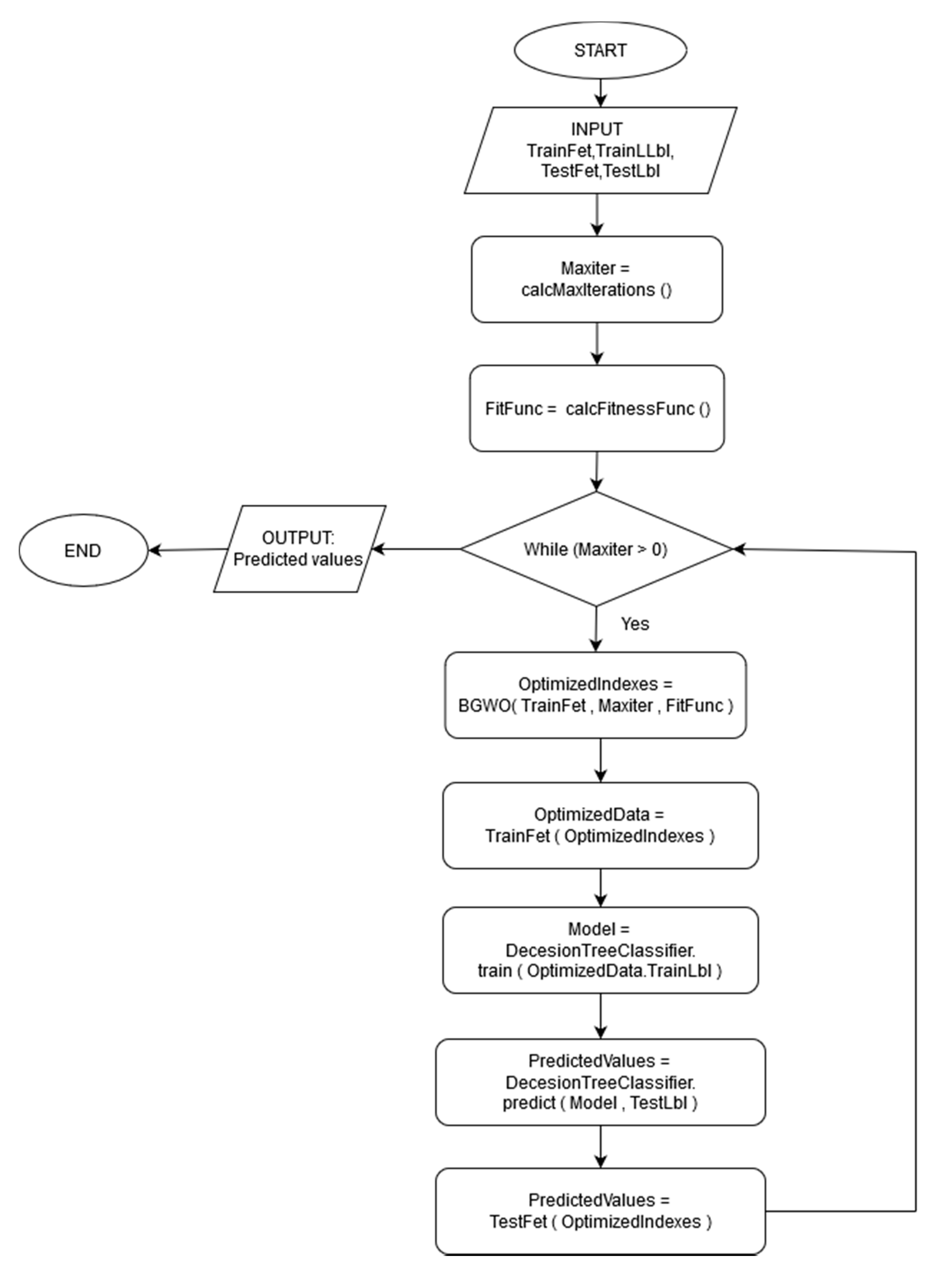
In this paper, three basic classifiers, along with optimization algorithms, were used to evaluate the proposed preprocessing and feature extraction methodology. These are the Decision Tree classifier optimized by BGWO, the SVM optimized by particle PSO, and the Genetic Algorithm optimized by ACO. Figure 7 defines the flowchart of feature optimization and classification.
3.4. Pre-Classification Using Binary Grey Wolf Optimization
Binary Grey Wolf Optimization (BGWO) is an optimization algorithm inspired by grey wolves that live in groups of 5 to 12 [30]. To estimate the leadership in an individual group, four levels named alpha, beta, delta, and omega are considered. Alpha includes the leaders of the individual group of males and females. Beta gives suggested feedback to the alpha when making decisions. Delta includes the roles of sentinels, elders, caretakers, and scouts. The omega wolves only obey other groups of wolves [31]. The BGWO algorithm is calculated as:
where Xp is the prey’s position vector. X mimics the position of wolves in n-dimensional space. r1 and r2 are random vectors that lie from 0 to 1 in each iteration. In the hunting process, alpha is the optimal solution, while beta and delta need to know the possible position of prey. Out of all possible solutions, only the three best possible solutions are selected to modify the decision space consistent with the best [32].
In BGWO, a is the main component of the algorithm. a is processed from increase to decrease vector of each dimension using the following formula to obtain the optimal solution [33]. The equation is defined as:
where t is the total number of iterations and maxiter is the maximum number of iterations in the optimization algorithm.
3.5. HAR Using a Decision Tree
The Decision Tree (DT) classifier [34] is commonly used as a predictive model for clustering, prediction, and recognition. A tree is built based on divide-and-rule, and certain parameters are applied to the DT to get the classification result.
The internal nodes of a DT are compared to the attribute values, and the decisions of the branches are made for the current node according to certain attribute conditions [35]. Finally, the leaf nodes provide conclusions. The above-defined process is repeated on a new node and forms a child of the root tree. Every non-leaf node is an input attribute of the sample data, and every leaf node is an output attribute of the sample data.
In a Decision Tree, each path from a root node to a leaf node resembles a set of attributes of conjunctions, while the tree itself represents the disjunction of these attributes of conjunctions [36]. Therefore, a DT is easily converted from IF-THEN statements to classification procedures and rules. The Decision Tree algorithm is described as follows.
3.5.1. Initialization of Attributes
In this case, every internal node is named attribute Ai. Every arc is marked as a predicate, which is applied to the corresponding attribute of the parent node. Finally, each node is named as a class as C1, C2, ..., and CN, respectively.
3.5.2. Classification and Prediction
A Decision Tree is built using training data, and this is commonly known as the induction of a decision tree. Classification and prediction methods are based on the given induction data matrix.
3.5.3. Building a DT from Training Data
To build a DT from training data, DT is built based on gain and gain ratio. The training data is divided into two classes Pi (acceptable level) and Ni (unacceptable level). The information needed to identify the classes of an element is made based on the following information.
The training set is partitioned based on features Xi. into different classes based on the weighted average. The Info(Pi,Ni) is represented with Info(TS) as follows:
Next, the information gain is calculated with the difference in the basis of features to identify the desired elements. The information gain on each element of the feature Xi is defined as:
The classification decisions are made based on the greatest value of the gain. Such a decision process is repeated until all the features are properly classified. Each node in DT is located with the greatest gain. The gain has a shortcoming effect, where the number of features is too big. To cope with this issue, the gain ratio is calculated based on gain information and split information. The split information is the split values of two classes Pi (acceptable level) and Ni (unacceptable level), which are represented with TS. The gain ratio is defined as:
A DT is a learning model that uses the information gain to evaluate a target node, and the complete function uses divide-and-rule, a no-return strategy, and a top-down approach. Every branch of a node subset acts recursively and builds Decision Tree nodes and leaves until the classification model is achieved [37]. The final result is shown in Figure 11.
4. Experimental Settings and Datasets
4.1. Dataset Description
A platform is established to evaluate the performance of the proposed methodology using a three-axis accelerometer and gyroscope. Wearable sensors are used to acquire human activity data, and the data are uploaded to signal processing software. Our algorithm can be applied in real-time situations, especially for the health care assessments of children and elderly people.
Three datasets were used in this experiment. The MOTIONSENSE dataset [38] is taken from the accelerometer and gyroscope sensors of an iPhone with a time constraint of 6 seconds. Six activities were performed by 24 participants in different manners, i.e., downstairs, jogging, going upstairs, sitting, walking, and standing.
The MHEALTH dataset [39] is an accelerometer, gyroscope, and magnetometer dataset. In this paper, only the accelerometer and gyroscope sensor data were used to evaluate the proposed model. The sensors were placed on the subject’s chest, right wrist, and left ankle. Twelve outdoor activities were performed, including walking, climbing stairs, standing still, sitting and relaxing, waist bending forward, cycling, jogging, running, jump forward and back, knees bending, frontal elevation of arms, and lying down.
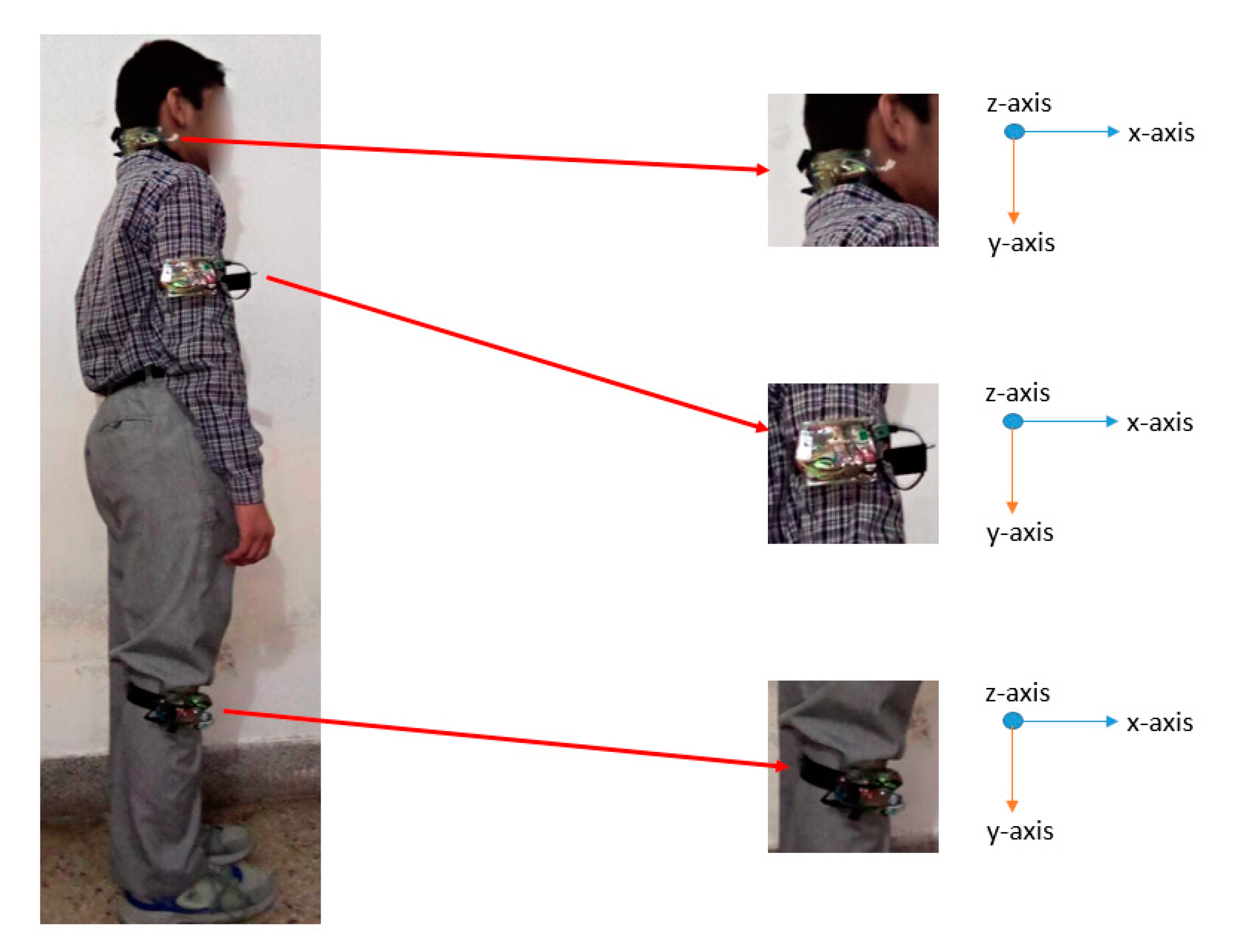
The IM-AccGyro dataset [40] is our self-annotated human–machine interactive dataset. Three accelerometer sensors were attached at three different locations, which were the arm, leg, and neck of the subject, as shown in Figure 10. The ages of the participants ranged from 15 to 30 years. Six different indoor and outdoor physical exercise activities were performed including boxing, walking, running, sitting-down, standing-up, and clapping.
4.2. Hardware Platform
In the experimental setup, the hardware platform comprised three GY-521 sensors. These sensors were interfaced with the Arduino device using jumper wires for electrical communication, and Bluetooth modules (HC-05) were also connected via GY-521 sensors. All the modules including GY-521, HC-05, and Arduino Uno along with a 9-Volt battery were fixed in a specially designed protective case that was then mounted on a belt and tied on the human body at the arm, leg, and neck position, as shown in Figure 12. Therefore, no sensor component would misbehave during the activities. The Bluetooth HC-05 transceiver modules were responsible for wireless communication and 9-Volt batteries were used with the setup to ensure uninterrupted data collection. The open-source Arduino software (IDE) was used to simulate operation in a real-time environment. During the trials, no loss of data occurred.
The GY-521 sensor provides six-degree-of-freedom (DOF) motion tracking. It consists of a three-axis accelerometer and a three-axis gyroscope embedded in a small chip, and it is based on a micro electro mechanical system (MEMS). The purpose of using the GY-521 sensor is its built-in digital motion processor (DMP) for motion processing. We received data angles of yaw, roll, and pitch with the GY-521. Thus, the burden of a host computer in the manipulation of motion data was minimized.
The limitation with the current setup is the 9-Volt battery. The power of the battery can operate the system for up to two days. There is a need to recharge or to replace the battery often to operate the prototype system for longer periods.
5. Experimental Results and Evaluation
The proposed system is evaluated using the “leave one subject out” (LOSO) cross-validation method with training and testing data. The three chosen classifiers with optimization algorithms are the following: the GA optimized by ACO, the DT optimized by wolf optimization, and the SVM optimized by PSO. The human activity classification algorithm is validated using precision, recall, and F-measure to identify different postures and movements. The precision is defined as the True positive (instances that belong to the class) by the total number of instances (True positive and False positive).
The recall is defined as the proportion of instances classified in one class by the total instances. Total instances include True Positive (TP) and True Negative (TN) values.
The F-measure is the combination of precision and recall and is defined as:
The classification results of the three classifiers, i.e., support vector machine, genetic algorithm, and decision tree on MOTIONSENSE, MHEALTH, and IM-AccGyro datasets are reported in Table 1, Table 2 and Table 3. All classifiers are trained on the training set. The classification results in Table 1, Table 2 and Table 3 were obtained by using the testing set. In Table 3, we got a better classification result on the IM-AccGyro dataset with an F-measure of more than 90% compared to the classification results of Table 1 and Table 2, i.e., the MOTIONSENSE, and MHEALTH datasets. The overall results showed that our proposed method achieved better performance than other state-of-the-art methods.
Table 4 depicts the confusion matrix of the MOTIONSENSE dataset for six different activities with a mean accuracy of 88.25%. Table 5 presents the mean accuracy of 93.95% on the MHEALTH dataset of 12 different activities. Table 6 shows the confusion matrix of the IM-AccGyro dataset for six different activities with an average accuracy of 96.83%. Table 7 presents the comparison results of the proposed approach over MOTIONSENSE, MHEALTH, and IM-AccGyro datasets, respectively.
6. Conclusions and Future Works
In this paper, we proposed a novel robust framework, called the multi combined features of the HAR system, which recognizes human activities via the inertial measurements captured from wearable sensors. The multi combined features examined the spatiotemporal variation, optimal pattern, structural uncertainty, rehabilitation motion, and transitional activity features. These features are then passed through three classifiers with optimization algorithms including the Genetic Algorithm (GA) optimized by Ant Colony Optimization (ACO), the Decision Tree (DT) optimized by Binary Grey Wolf Optimization (BGWO), and the Support Vector Machine (SVM) optimized by Particle Swarm Optimization (PSO). During the experiments, we used three challenging inertial sensors datasets including the MOTIONSENSE, MHEALTH, and a proposed self-annotated IM-AccGyro human–machine dataset. The recent work done by numerous researchers using state-of-the-art classifiers (SVM [41] and GA [42]) has shown good classification results against multiple benchmark HAR datasets. That is why we evaluated our proposed model against these classifiers. Our proposed method achieved remarkable recognition accuracy performance over the state-of-the-art methods.
As future work, we will improve the efficiency of our multi combined features by adding wavelet and frequency-domain features. Additionally, we are planning to develop more complex activities for different scenarios such as smart homes, offices, and hospitals using various other wearable sensors.
Author Contributions
Conceptualization, M.B.; methodology, M.B. and A.J.; software, M.B.; validation, A.J.; formal analysis, K.K.; resources, A.J. and K.K.; writing—review and editing, A.J. and K.K.; funding acquisition, A.J. and K.K. All authors have read and agreed to the published version of the manuscript.
Funding
This research was supported by the Basic Science Research Program through the National Research Foundation of Korea (NRF), funded by the Ministry of Education (No. 2018R1D1A1A02085645) and by a grant (19CTAP-C152247-01) from the Technology Advancement Research Program funded by the Ministry of Land, Infrastructure and Transport of the Korean government.
Conflicts of Interest
The authors declare no conflict of interest.
References
- Ronao, C.A.; Cho, S.B. Human activity recognition with smartphone sensors using deep learning neural networks. Expert Syst. Appl. 2016, 59, 235–244. [Google Scholar] [CrossRef]
- Mahmood, M.; Jalal, A.; Kim, K. WHITE STAG Model: Wise Human Interaction Tracking and Estimation (WHITE) using Spatio-temporal and Angular-geometric (STAG) Descriptors. Multimed. Tools Appl. 2020, 79, 6919–6950. [Google Scholar] [CrossRef]
- Sharma, R.; Ribeiro, B.; Pinto, A.M.; Cardoso, F.A. Exploring Geometric Feature Hyper-Space in Data to Learn Representations of Abstract Concepts. Appl. Sci. 2020, 10, 1994. [Google Scholar] [CrossRef] [Green Version]
- Alsheikh, M.A.; Selim, A.; Niyato, D.; Doyle, L.; Lin, S.; Tan, H.P. Deep activity recognition models with triaxial accelerometers. In Proceedings of the Workshops at the Thirtieth AAAI Conference on Artificial Intelligence, Phoenix, AZ, USA, 12–13 February 2016. [Google Scholar]
- Shokri, M.; Tavakoli, K. A review on the artificial neural network approach to analysis and prediction of seismic damage in infrastructure. Int. J. Hydromechatron. 2019, 4, 178–196. [Google Scholar] [CrossRef]
- Osterland, S.; Weber, J. Analytical analysis of single-stage pressure relief valves. Int. J. Hydromechatron. 2019, 2, 32–53. [Google Scholar] [CrossRef]
- Nizami, I.F.; Majid, M.; ur Rehman, M.; Anwar, S.M.; Nasim., A.; Khurshid , K. No-reference image quality assessment using bag-of-features with feature selection. Multimed. Tools Appl. 2020, 79, 7811–7836. [Google Scholar] [CrossRef]
- Jalal, A.; Khalid, N.; Kim, K. Automatic Recognition of Human Interaction via Hybrid Descriptors and Maximum Entropy Markov Model Using Depth Sensors. Entropy 2020, 22, 817. [Google Scholar] [CrossRef]
- Susan, S.; Agrawal, P.; Mittal, M.; Bansal, S. New shape descriptor in the context of edge continuity. CAAI Trans. Intell. Technol. 2019, 4, 101–109. [Google Scholar] [CrossRef]
- Jalal, A.; Kim, Y.-H.; Kim, Y.-J.; Kamal, S.; Kim, D. Robust human activity recognition from depth video using spatiotemporal multi-fused features. Pattern Recognit. 2017, 61, 295–308. [Google Scholar] [CrossRef]
- Yang, J.B.; Nguyen, M.N.; San, P.P.; Li, X.L.; Krishnaswamy, S. Deep convolutional neural networks on multichannel time series for human activity recognition. In Proceedings of the 24th International Conference on Artificial Intelligence (IJCAI 15), Buenos Aires, Argentina, 25–31 July 2015. [Google Scholar]
- Tingting, Y.; Junqian, W.; Lintai, W.; Yong, X. Three-stage network for age estimation. CAAI Trans. Intell. Technol. 2019, 4, 122–126. [Google Scholar] [CrossRef]
- Iglesias, J.A.; Ledezma, A.; Sanchis, A.; Angelov, P. Real-Time Recognition of Calling Pattern and Behaviour of Mobile Phone Users through Anomaly Detection and Dynamically-Evolving Clustering. Appl. Sci. 2017, 7, 798. [Google Scholar] [CrossRef] [Green Version]
- Sargano, A.B.; Angelov, P.; Habib, Z. A Comprehensive Review on Handcrafted and Learning-Based Action Representation Approaches for Human Activity Recognition. Appl. Sci. 2017, 7, 110. [Google Scholar] [CrossRef] [Green Version]
- Wiens, T. Engine speed reduction for hydraulic machinery using predictive algorithms. Int. J. Hydromechatron. 2019, 1, 16–31. [Google Scholar] [CrossRef]
- Babiker, M.; Khalifa, O.O.; Htike, K.K.; Hassan, A.; Zaharadeen, M. Automated daily human activity recognition for video surveillance using neural network. In Proceedings of the IEEE 4th International Conference on Smart Instrumentation, Measurement and Application (ICSIMA), Putrajaya, Malaysia, 28–30 November 2017. [Google Scholar]
- Jalal, A.; Uddin, M.Z.; Kim, T.S. Depth Video-based Human Activity Recognition System Using Translation and Scaling Invariant Features for Life Logging at Smart Home. IEEE Trans. Consum. Electron. 2012, 58, 3. [Google Scholar] [CrossRef]
- Liu, L.; Peng, Y.X.; Liu, M.; Lukowicz, P. Sensor-based human activity recognition system with a multilayered model using time series shapelets. Knowl. Based Syst. 2015, 90, 138–152. [Google Scholar] [CrossRef]
- Jansi, R.; Amutha, R. Sparse representation based classification scheme for human activity recognition using smartphones. Multimed. Tools Appl. 2018, 78, 11027–11045. [Google Scholar] [CrossRef]
- Tian, Y.; Wang, X.; Chen, L.; Liu, Z. Wearable Sensor-Based Human Activity Recognition via Two-Layer Diversity-Enhanced Multiclassifier Recognition Method. Sensors 2019, 19, 2039. [Google Scholar] [CrossRef] [Green Version]
- Tahir, S.B.; Jalal, A.; Kim, K. Wearable Inertial Sensors for Daily Activity Analysis Based on Adam Optimization and the Maximum Entropy Markov Model. Entropy 2020, 22, 579. [Google Scholar] [CrossRef]
- Haresamudram, H.; Beedu, A.; Agrawal, V.; Grady, P.L.; Essa, I. Masked Reconstruction Based Self-Supervision for Human Activity Recognition. In Proceedings of the 24th annual International Symposium on Wearable Computers, Cancun, Mexico, 12–16 September 2020. [Google Scholar]
- Jordao, A.; Nazare, A.C.; Sena, J.; Schwartz, W.R. Human Activity Recognition Based on Wearable Sensor Data: A Standardization of the State-of-the-Art. arXiv 2019, arXiv:1806.05226. [Google Scholar]
- Batool, M.; Jalal, A.; Kim, K. Sensors Technologies for Human Activity Analysis Based on SVM Optimized by PSO Algorithm. In Proceedings of the 2019 International Conference on Applied and Engineering Mathematics (ICAEM), Taxila, Pakistan, 27–29 August 2019. [Google Scholar]
- Zha, Y.B.; Yue, S.G.; Yin, Q.J.; Liu, X.C. Activity recognition using logical hidden semi-markov models. In Proceedings of the 2013 10th International Computer Conference on Wavelet Active Media Technology and Information Processing (ICCWAMTIP), Chengdu, China, 17–19 December 2013. [Google Scholar]
- Zhu, C.; Miao, D. Influence of kernel clustering on an RBFN. CAAI Trans. Intell. Technol. 2019, 4, 255–260. [Google Scholar] [CrossRef]
- Nakano, K.; Chakraborty, B. Effect of Dynamic Feature for Human Activity Recognition using Smartphone Sensors. In Proceedings of the 2017 IEEE 8th International Conference on Awareness Science and Technology (iCAST), Taichung, Taiwan, 8–10 November 2017. [Google Scholar]
- Hamad, R.A.; Yang, L.; Woo, W.L.; Wei, B. Joint Learning of Temporal Models to Handle Imbalanced Data for Human Activity Recognition. Appl. Sci. 2020, 10, 5293. [Google Scholar] [CrossRef]
- Rodriguez, M.D.; Ahmed, J.; Shah, M. Action MACH: A spatio-temporal maximum average correlation height filter for action recognition. Computer Vision and Pattern Recognition. In Proceedings of the 2008 IEEE conference on computer vision and pattern recognition, Anchorage, AK, USA, 23–28 June 2008. [Google Scholar]
- Zhu, J.; San-Segundo, R.; Pardo, J.M. Feature extraction for robust physical activity recognition. Hum. Cent. Comput. Inf. Sci. 2017, 7, 219. [Google Scholar] [CrossRef] [Green Version]
- Biel, L.; Pettersson, O.; Philipson, L.; Wide, P. ECG analysis: A new approach in human identification. IEEE Trans. Instrum. Meas. 2001, 50, 808–812. [Google Scholar] [CrossRef] [Green Version]
- Tashi, Q.A.; Kadir, S.J.A.; Rais, H.M.; Mirjalili, S.; Alhussian, H. Binary Optimization Using Hybrid Grey Wolf Optimization for Feature Selection. IEEE Access 2019, 7, 39496–39508. [Google Scholar] [CrossRef]
- Jiang, K.; Ni, H.; Sun, P.; Han, R. An Improved Binary Grey Wolf Optimizer for Dependent Task Scheduling in Edge Computing. In Proceedings of the 2019 21st International Conference on Advanced Communication Technology (ICACT), PyeongChang, Korea, 17–20 February 2019. [Google Scholar]
- Mirjalili, S.; Mirjalili, S.M.; Lewis, A. Grey wolf optimizer. Adv. Eng. Softw. 2014, 69, 46–61. [Google Scholar] [CrossRef] [Green Version]
- Emary, E.; Hossam, M. Binary grey wolf optimization approaches for feature selection. Neurocomputing 2016, 172, 371–381. [Google Scholar] [CrossRef]
- Yin, D.S.; Wang, G.Y. A Self Learning Algorithm for Decision Tree Pre-prunning. In Proceedings of the 2004 International Conference on Machine Learning and Cybernetics, Shanghai, China, 26–29 August 2004. [Google Scholar]
- Ling, C.X.; Sheng, V.S.; Yang, Q. Test Strategies for Cost Sensitive Decision Trees. IEEE Trans. Knowl. Data Eng. 2006, 18, 8. [Google Scholar] [CrossRef] [Green Version]
- Malekzadeh, M.; Clegg, R.G.; Cavallaro, A.; Haddadi, H. Mobile Sensor Data Anonymization. In Proceedings of the International Conference on Internet of Things Design and Implementation, Montreal, QC, Canada, 15–18 April 2019. [Google Scholar]
- Banos, O.; Garcia, R.; Holgado-Terriza, J.A.; Damas, M.; Pomares, H.; Rojas, I.; Saez, A.; Villalonga, C. mHealthDroid: A novel framework for agile development of mobile health applications. In Proceedings of the 6th International Work-conference, Belfast, UK, 2–5 December 2014. [Google Scholar]
- Intelligent Media Center (IMC). Available online: https://github.com/Mouazma/IM-AccGyro (accessed on 15 September 2020).
- Guo, M.; Wang, W.; Yang, N.; Li, Z.; An, T. A multisensor multiclassifier hierarchical fusion model based on entropy weight for human activity recognition using wearable inertial sensors. IEEE Trans. Hum. Mach. Syst. 2018, 49, 105–111. [Google Scholar] [CrossRef]
- Fan, S.; Jia, Y.; Jia, C. A Feature Selection and Classification Method for Activity Recognition Based on an Inertial Sensing Unit. Information 2019, 10, 290. [Google Scholar] [CrossRef] [Green Version]
Figure 1.
Flow architecture of the proposed methodology for human activity recognition.

Figure 2.
Band-stop filtration of the accelerometer data in the preprocessing step. The red and blue signals represent the filtered data and the unfiltered data, respectively.
Figure 2.
Band-stop filtration of the accelerometer data in the preprocessing step. The red and blue signals represent the filtered data and the unfiltered data, respectively.

Figure 3.
Flowchart of the human locomotion feature extraction process.

Figure 4.
Means, medians, and harmonic means of data samples. The blue and red dots represent the sitting down data and the standing up data taken from the accelerometer.
Figure 4.
Means, medians, and harmonic means of data samples. The blue and red dots represent the sitting down data and the standing up data taken from the accelerometer.

Figure 5.
Cosine coefficients of football and basketball activities. The cosine coefficients of the football and basketball activities signal are depicted by blue and purple signals.
Figure 5.
Cosine coefficients of football and basketball activities. The cosine coefficients of the football and basketball activities signal are depicted by blue and purple signals.

Figure 6.
The position vectors of running and walking activities. The position vectors of running and of walking activities are represented with the purple and the green dotted lines.
Figure 6.
The position vectors of running and walking activities. The position vectors of running and of walking activities are represented with the purple and the green dotted lines.

Figure 7.
Flowchart of human locomotion feature optimization and classification.

Figure 8.
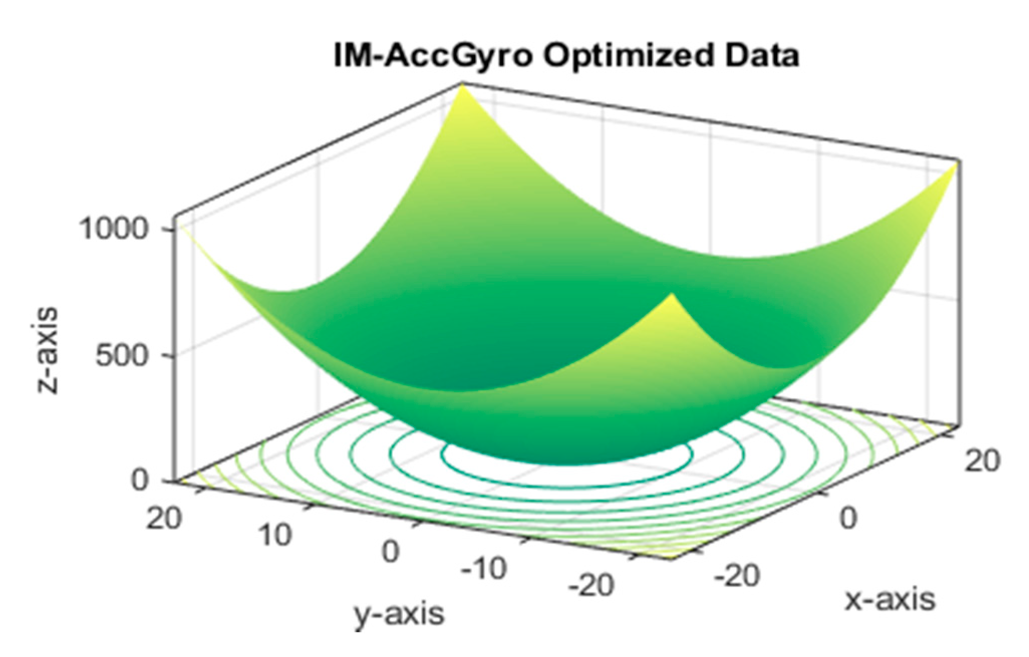
Convergence of IM-AccGyro optimized data along the x, y and z axes.

Figure 9.
Convergence of MHEALTH optimized data along the x, y and z axes.

Figure 10.
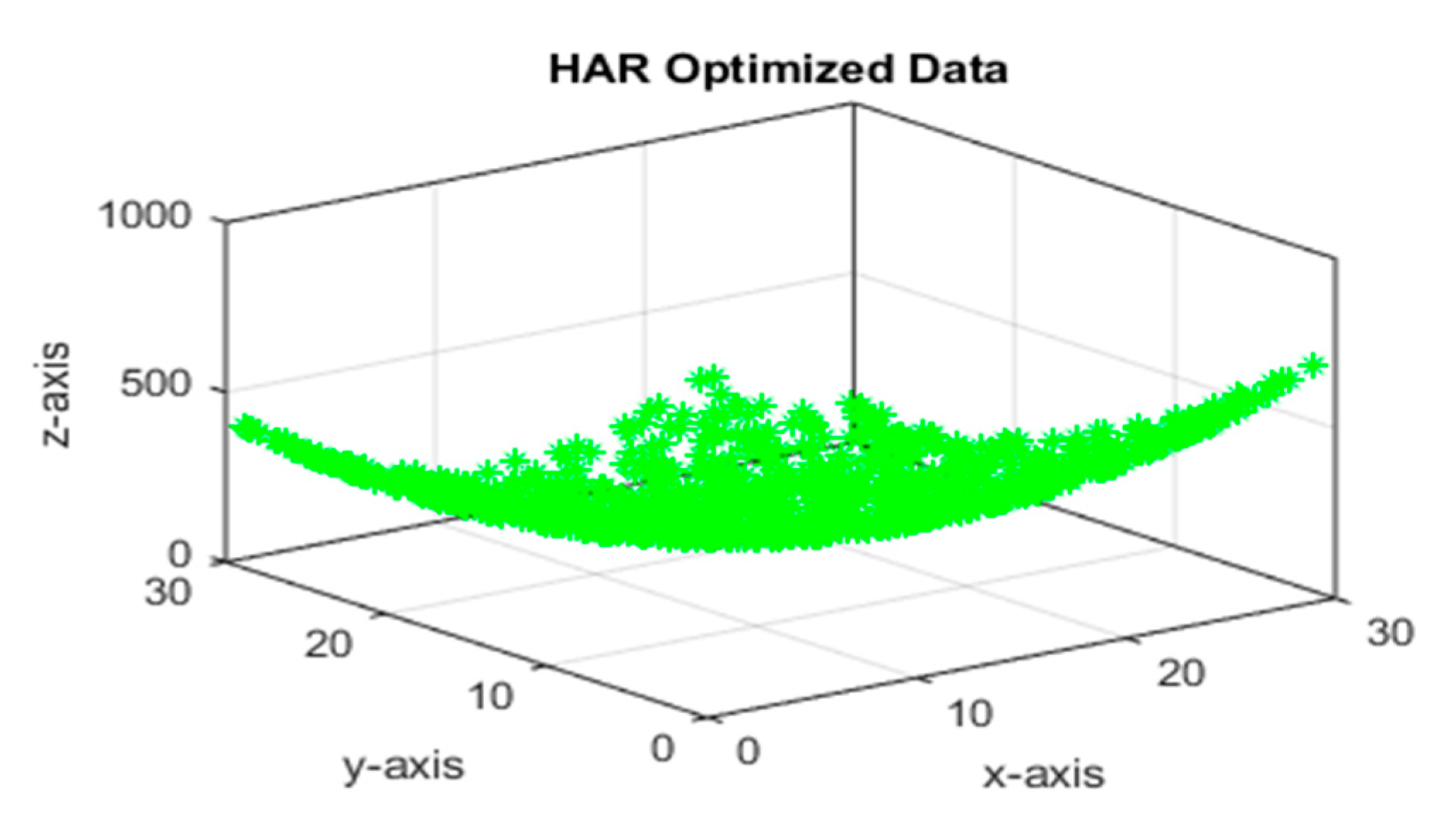
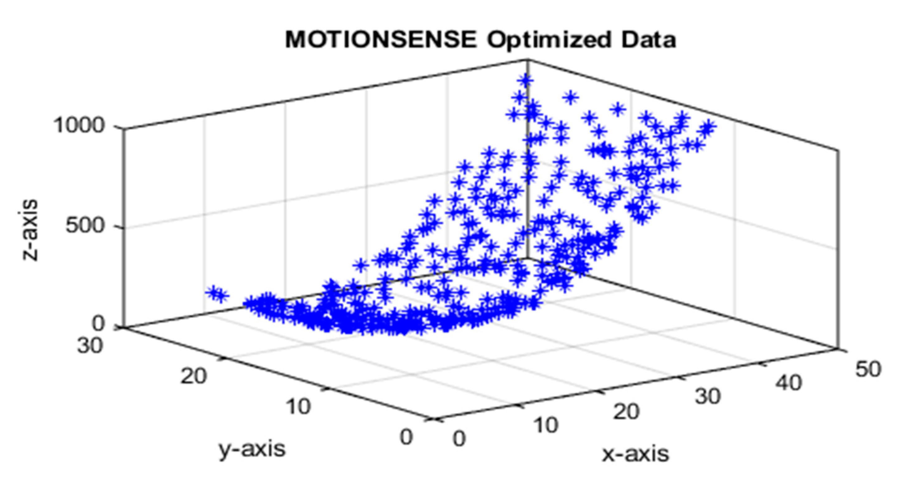
Convergence of MOTIONSENSE optimized data along the 3D axes.

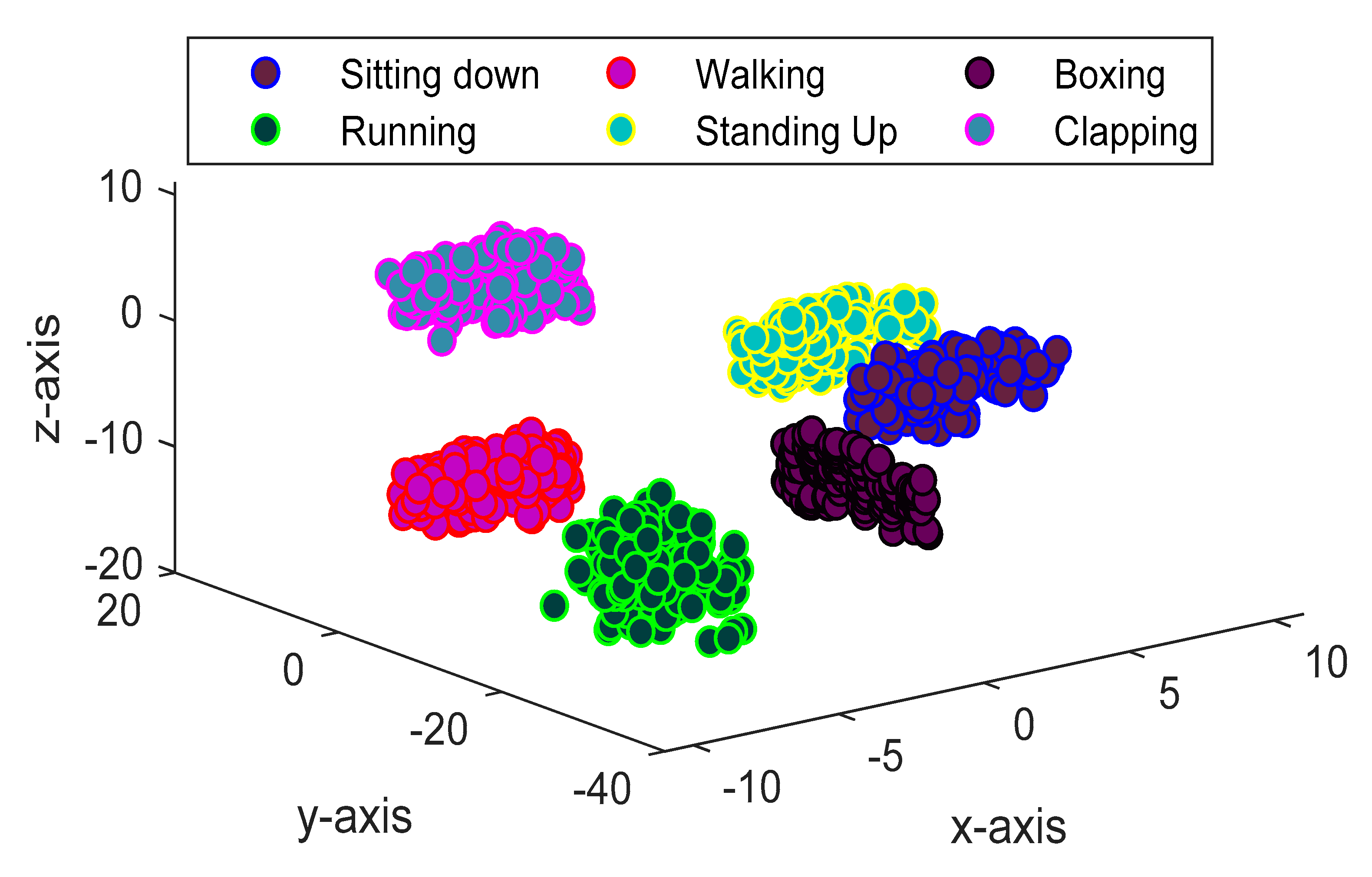
Figure 11.
Classification result of the Decision Tree algorithm on the IM-AccGyro dataset.

Figure 12.
Placement of the sensors on the human body at the leg, neck, and arm positions for data acquisition of the self-annotated IM-AccGyro human–machine dataset.
Figure 12.
Placement of the sensors on the human body at the leg, neck, and arm positions for data acquisition of the self-annotated IM-AccGyro human–machine dataset.


Table 1.
The classification results of three classifiers on the MOTIONSENSE dataset.
| Dynamic Activities | Support Vector Machine | Genetic Algorithm | Decision Tree | ||||||
|---|---|---|---|---|---|---|---|---|---|
| Activities | Precision | Recall | F-measure | Precision | Recall | F-measure | Precision | Recall | F-measure |
| DWS | 0.860 | 0.830 | 0.844 | 0.910 | 0.875 | 0.892 | 0.927 | 0.890 | 0.908 |
| UPS | 0.843 | 0.878 | 0.860 | 0.873 | 0.838 | 0.855 | 0.989 | 0.985 | 0.987 |
| WLK | 0.884 | 0.849 | 0.866 | 0.809 | 0.834 | 0.821 | 0.807 | 0.880 | 0.842 |
| JOG | 0.908 | 0.873 | 0.890 | 0.925 | 0.890 | 0.907 | 0.820 | 0.845 | 0.832 |
| SIT | 0.853 | 0.818 | 0.835 | 0.844 | 0.869 | 0.856 | 0.895 | 0.860 | 0.877 |
| STD | 0.882 | 0.937 | 0.908 | 0.854 | 0.829 | 0.841 | 0.865 | 0.835 | 0.849 |
DWS = Downstairs, UPS = Upstairs, WLK = Walking, JOG = Jogging, SIT = Sitting, STD = Standing.
Table 2.
The classification results of three classifiers on the MHEALTH dataset.
| Dynamic Activities | Support Vector Machine | Genetic Algorithm | Decision Tree | ||||||
|---|---|---|---|---|---|---|---|---|---|
| Activities | Precision | Recall | F-measure | Precision | Recall | F-measure | Precision | Recall | F-measure |
| WLK | 0.867 | 0.907 | 0.886 | 0.858 | 0.891 | 0.874 | 0.918 | 0.960 | 0.938 |
| CLS | 0.968 | 0.873 | 0.918 | 0.836 | 0.876 | 0.855 | 0.953 | 0.925 | 0.939 |
| STS | 0.882 | 0.977 | 0.927 | 0.818 | 0.858 | 0.837 | 0.933 | 0.985 | 0.958 |
| STR | 0.874 | 0.834 | 0.853 | 0.932 | 0.892 | 0.911 | 0.905 | 0.955 | 0.929 |
| WBF | 0.843 | 0.884 | 0.863 | 0.912 | 0.872 | 0.891 | 0.949 | 0.935 | 0.942 |
| CYC | 0.890 | 0.931 | 0.910 | 0.956 | 0.816 | 0.880 | 0.963 | 0.930 | 0.946 |
| JOG | 0.876 | 0.836 | 0.855 | 0.857 | 0.814 | 0.834 | 0.928 | 0.970 | 0.948 |
| RUN | 0.962 | 0.933 | 0.947 | 0.909 | 0.869 | 0.888 | 0.965 | 0.965 | 0.965 |
| JFB | 0.877 | 0.846 | 0.861 | 0.806 | 0.848 | 0.826 | 0.919 | 0.975 | 0.946 |
| KNB | 0.947 | 0.987 | 0.966 | 0.965 | 0.925 | 0.944 | 0.966 | 0.860 | 0.910 |
| FEA | 0.855 | 0.894 | 0.874 | 0.879 | 0.839 | 0.858 | 0.936 | 0.888 | 0.911 |
| LYD | 0.943 | 0.911 | 0.926 | 0.952 | 0.915 | 0.933 | 0.954 | 0.935 | 0.944 |
WLK = Walking, CLS = Climbing stairs, STS = Standing still, STR = Sitting & relaxing, WBF = Waist bend forward, CYC = Cycling, JOG = Jogging, RUN = Running, JFB = Jump front & back, KNB = Knees bending, FEA = Frontal elevation of arms, LYD = Lying down.
Table 3.
The classification results of three classifiers on the IM-AccGyro dataset.
| Dynamic Activities | Support Vector Machine | Genetic Algorithm | Decision Tree | ||||||
|---|---|---|---|---|---|---|---|---|---|
| Activities | Precision | Recall | F-measure | Precision | Recall | F-measure | Precision | Recall | F-measure |
| STU | 0.907 | 0.900 | 0.903 | 0.906 | 0.913 | 0.909 | 0.945 | 0.955 | 0.950 |
| WLK | 0.921 | 0.928 | 0.924 | 0.911 | 0.904 | 0.907 | 0.970 | 0.970 | 0.970 |
| CLP | 0.917 | 0.910 | 0.913 | 0.919 | 0.912 | 0.915 | 0.980 | 0.985 | 0.982 |
| BOX | 0.912 | 0.905 | 0.908 | 0.916 | 0.923 | 0.919 | 0.989 | 0.945 | 0.966 |
| RUN | 0.915 | 0.922 | 0.918 | 0.908 | 0.902 | 0.904 | 0.970 | 0.990 | 0.980 |
| STD | 0.913 | 0.906 | 0.909 | 0.921 | 0.914 | 0.917 | 0.955 | 0.965 | 0.960 |
STU = Standing Up, WLK = Walking, CLP = Clapping, BOX = Boxing, RUN = Running, STD = Sitting Down.
Table 4.
Confusion matrix of MOTIONSENSE dataset.
| Dynamic Activities | DWS | JOG | UPS | SIT | WLK | STD |
|---|---|---|---|---|---|---|
| DWS | 89.00 | 1.00 | 5.50 | 0 | 4.50 | 0 |
| JOG | 0 | 98.50 | 0 | 1.50 | 0 | 0 |
| UPS | 0 | 0 | 88.00 | 9.50 | 0 | 2.50 |
| SIT | 0 | 0 | 15.50 | 84.50 | 0 | 0 |
| WLK | 3.50 | 0 | 0 | 0 | 86.0 | 10.50 |
| STD | 3.50 | 0 | 0 | 7.50 | 5.50 | 83.50 |
| Mean Accuracy = 88.25% | ||||||
Table 5.
The classification results of three classifiers on the MHEALTH dataset.
| Dynamic Activities | WLK | CLS | STS | STR | WBF | CYC | JOG | RUN | JFB | KNB | FEA | LYD |
|---|---|---|---|---|---|---|---|---|---|---|---|---|
| WLK | 96.00 | 0 | 0 | 0 | 0 | 0 | 0 | 2.50 | 1.50 | 0 | 0 | 0 |
| CLS | 0 | 92.50 | 1.50 | 1.50 | 0.50 | 0.50 | 0.50 | 0.50 | 0 | 2.50 | 0 | 0 |
| STS | 0 | 0 | 98.50 | 0 | 0 | 0 | 0 | 0 | 0 | 0 | 0 | 1.50 |
| STR | 0.50 | 0 | 0 | 95.50 | 0 | 0 | 0 | 0 | 0 | 0 | 2.50 | 1.50 |
| WBF | 0 | 0 | 2.50 | 0 | 93.50 | 0 | 0 | 0 | 3.50 | 0 | 0 | 0.50 |
| CYC | 0 | 2.50 | 0.50 | 0 | 0 | 93.00 | 0 | 0.50 | 1.00 | 0 | 2.50 | 0 |
| JOG | 0 | 0.50 | 0 | 0 | 0 | 1.50 | 97.00 | 0 | 0.50 | 0 | 0.50 | 0 |
| RUN | 0 | 0 | 0 | 2.50 | 0.50 | 0 | 0 | 96.50 | 0 | 0 | 0.50 | 0 |
| JFB | 0 | 0 | 0 | 0 | 0 | 0 | 2.50 | 0 | 97.50 | 0 | 0 | 0 |
| KNB | 5.50 | 0 | 0 | 3.50 | 4.00 | 0 | 0.50 | 0 | 0 | 86.00 | 0 | 0.50 |
| FEA | 2.50 | 1.50 | 2.50 | 0 | 0 | 1.00 | 0.50 | 0 | 2.00 | 0.50 | 88.0 | 0.50 |
| LYD | 0 | 0 | 0 | 2.50 | 0 | 0.50 | 3.50 | 0 | 0 | 0 | 0 | 93.50 |
| Mean Accuracy = 93.95% | ||||||||||||
Table 6.
Confusion matrix of IM-AccGyro dataset.
| Dynamic Activities | STU | WLK | CLP | BOX | RUN | STD |
|---|---|---|---|---|---|---|
| STU | 95.50 | 0 | 0 | 0 | 0 | 4.50 |
| WLK | 2.50 | 97.00 | 0 | 0 | 0.50 | 0 |
| CLP | 0 | 0 | 98.50 | 1.00 | 0.50 | 0 |
| BOX | 0 | 2.50 | 1.00 | 94.50 | 2.00 | 0 |
| RUN | 0 | 0.50 | 0.50 | 0 | 99.00 | 0 |
| STD | 3.00 | 0 | 0.50 | 0 | 0 | 96.50 |
| Mean Accuracy = 96.83% | ||||||
© 2020 by the authors. Licensee MDPI, Basel, Switzerland. This article is an open access article distributed under the terms and conditions of the Creative Commons Attribution (CC BY) license (http://creativecommons.org/licenses/by/4.0/).
Share and Cite
MDPI and ACS Style
Jalal, A.; Batool, M.; Kim, K. Stochastic Recognition of Physical Activity and Healthcare Using Tri-Axial Inertial Wearable Sensors. Appl. Sci. 2020, 10, 7122. https://0-doi-org.brum.beds.ac.uk/10.3390/app10207122
AMA Style
Jalal A, Batool M, Kim K. Stochastic Recognition of Physical Activity and Healthcare Using Tri-Axial Inertial Wearable Sensors. Applied Sciences. 2020; 10(20):7122. https://0-doi-org.brum.beds.ac.uk/10.3390/app10207122
Chicago/Turabian StyleJalal, Ahmad, Mouazma Batool, and Kibum Kim. 2020. "Stochastic Recognition of Physical Activity and Healthcare Using Tri-Axial Inertial Wearable Sensors" Applied Sciences 10, no. 20: 7122. https://0-doi-org.brum.beds.ac.uk/10.3390/app10207122
Note that from the first issue of 2016, this journal uses article numbers instead of page numbers. See further details here.