Article

Experimental Investigation on Glaze Ice Accretion and Its Influence on Aerodynamic Characteristics of Pipeline Suspension Bridges

1
School of Civil Engineering, Dalian University of Technology, Dalian 116024, China
2
Department of Structural Engineering, Norwegian University of Science and Technology, 7491 Trondheim, Norway
*
Author to whom correspondence should be addressed.
Submission received: 21 September 2020 / Revised: 8 October 2020 / Accepted: 10 October 2020 / Published: 14 October 2020
(This article belongs to the Special Issue Advances on Structural Engineering, Volume II)

Abstract

:
Pipeline suspension bridges may experience ice accretion under special atmospheric conditions, and the aerodynamic characteristics of the bridges may be modified by the ice accretion. Under some specific climatic conditions of freezing rain, the dependencies of the ice size and shape on the icing duration and some structural properties (including pipeline diameter, inclination angle of wind hanger, inclination angle and size of section steel, and girder geometry) were experimentally investigated in a refrigerated precipitation icing laboratory. Typical ice accretions on pipelines, wind hangers, section steels, and girders of pipeline suspension bridges are summarized. Then the effects of some selected ice accretions on aerodynamic force coefficients of a bridge girder were further investigated through wind tunnel tests. The ice size and shape on the pipeline were closely related to the pipeline diameter and icing duration. The engineering geometric models of ice accretion on pipelines were extracted. The ice shape and size on wind hangers and section steels changed with their inclination angles. The aerodynamic force coefficients of a girder with ice accretion were much higher than those of an ice-free one. The results can provide references for simulating the ice accretion and further evaluating the effect of ice accretion on the aerodynamics of pipeline suspension bridges.

1. Introduction

Pipeline bridges carry pipelines of natural gas, oil, or water across rivers, canyons, or other natural or man-made obstacles. Pipeline bridges are mainly designed as suspension bridges for cases with main span lengths over 200 m. Compared with highway suspension bridges, pipeline suspension bridges are much narrower, blunter, lighter, and more flexible, and thus, they are highly sensitive to wind action. As a result, wind loads should be carefully addressed to ensure the safety of a pipeline suspension bridge. If the pipeline is damaged by strong winds, the oil or gas will leak out, which can even result in catastrophic fire or explosion disasters. This would not only cause significant economic losses but also lead to heavy casualties and significant secondary environmental pollution. A natural gas pipeline exploded in the southeast of New Mexico in August 2000. Twelve people were killed, and two nearby pipelines bridges were severely damaged in the accident [1]. In November 2013, an oil pipeline exploded in Qingdao, China, and the blast killed 62 people [2].
In the forthcoming two decades, the construction of pipeline networks will be promoted in Southwest China (e.g., Yunnan and Guizhou province). Unfortunately, glaze ice accretion may occur in these regions, for example, the freezing rain and snowstorm event at the beginning of 2008 in southern China. As a result, pipeline suspension bridges will confront the issue of ice accretion. Until now, a large number of investigations have shown that glaze ice accretion can modify the aerodynamic force coefficients of a circular cylinder (which may represents a transmission line, a bridge hanger, or a stay cable) and induce galloping due to the change of the aerodynamic shape, and ice accretion may also lead to structural failures due to the self-weight of the ice [3,4,5,6,7,8,9,10]. The cross sections of pipeline suspension bridges (including the truss stiffening girder, pipeline, grate plate, and guardrail) are much more complicated than circular cylinders. The findings of previous studies cannot be directly used to design and maintain pipeline suspension bridges. Therefore, it is necessary to evaluate the effects of ice accretion on the aerodynamic properties of pipeline suspension bridges.
Investigation of ice accretion is the first step toward studying its effect on the aerodynamic response of a structure [11,12]. Recently, some studies focused on the glaze ice accretion on circular cylinders [7,13,14,15,16,17,18], insulators [19,20], airfoils [21,22], and wind turbine blades [23,24]. The accreted ice mass and the detailed shapes were studied. The radial ice accretion on circular cylinder was most widely studied in the literatures, and ice accretion model of a circular cylinder can be simulated as follows: (1) the simplified ice shape, including triangle shape, crescent shape, ellipse shape, D-shape, sector-shape, and so on (as shown in Figure 1, the first four ice shapes are more common in power transmission lines, and the latter three ice shapes are more common in stay cables), was covered on the circular cylinder, which was extracted based on icing tests or field observations [4,9,14,18,25,26,27,28]; (2) the complicated artificial ice model was obtained by 3D scanning and printing technology [29]; (3) the real ice model was acquired in the icing wind tunnel [5,7,15].
The ice shapes on pipeline suspension girders may be very different from those in the abovementioned objects. In addition, some experimental results demonstrated that the ice shape is dependent on the cylinder diameter D. Jones [30] showed that the uniform radial ice thickness of the circular cylinder is related to its diameter based on a precipitation model, and ice shape depends on the diameter of the wire. Koss et al. [14] experimentally investigated the ice accretion on circular cylinders (D = 38.1 and 89 mm) and showed that the thermodynamic solidification processes and ice surface characteristics are related to the diameter. Otherwise, Langmuir et al. [31] and Finstad et al. [32] showed that the droplet collision efficiency significantly decreases with increasing D in in-cloud icing. The pipeline diameters (300–1000 mm) of suspension bridges are generally much larger than those examined in the abovementioned studies (D ≤ 160 mm). Hence, those ice accretion shapes may be inappropriate for the pipeline. For this reason, it is necessary to further investigate the ice accretion shapes on pipelines over a wider range of diameters.
To compensate for the lack of experimental data on the ice accretion on pipeline suspension bridges, a series of ice accretion tests during freezing rain were undertaken in a refrigerated precipitation icing laboratory. The dependencies of the ice size and shape on the icing duration and some structural properties (including pipeline diameter, inclination angle of wind hanger, inclination angle and size of section steel, and girder geometry) were experimentally investigated. Then the effects of some selected ice accretions on aerodynamic force coefficients of a pipeline bridge girder were further investigated through wind tunnel tests.

2. Ice Accretion Tests

To investigate the characteristics of the ice accretion on a pipeline, wind hanger, section steel, and typical section model of pipeline suspension bridges, a series of experiments were carried out in the Refrigerated Precipitation Icing Laboratory in Dalian University of Technology. The facilities, testing procedures, testing cases, and measurements of ice accretion are described in this section.

2.1. Facilities and Experimental Procedure

The laboratory had a work section with dimensions of 4.7 m (length), 3.7 m (width), and 2.6 m (height). The temperature T in the testing zone could be adjusted continuously between −20 and 20 °C with an accuracy of ±0.1 °C which was controlled and measured by a thermostat. Icing objects were supported on the steel brackets, as shown in Figure 2. Several air-atomizing nozzles were used to spray water to simulate the required rainfall intensity and environmental humidity. The vertical distances between atomizing nozzles and the top surface of icing objects were about 50 cm.
Generally, the range of the mean volume diameter (MVD) in freezing rain is from 500 μm to 3–4 mm [33]. The diameters of the sprinkler heads were 2.0 mm. Huffman et al. [34] showed that freezing rain is generally produced at temperatures ranging from 0 °C to −10 °C. The laboratory air temperature was set to −7 °C to accelerate the icing progress. The average humidity was set to around 80% at the position of icing objects based on the results of Jiang and Yi [35]. Freezing rain was reproduced in the tests, the precipitation rate in freezing rain is usually 1–2 mm/h, and in extreme cases 10 mm/h [30]. Unfortunately, the precipitation rate was set 45 mm/h in the experiment which was much higher than typical values encountered during freezing rain to hasten the icing process by referring to the recommend values 60 ± 20 mm/h in Farzaneh et al. [19]. It was impossible to produce more typical freezing rainfall rates of 1 mm/h without compromising the uniformity of the water supply along the cylinder [16]. Water was chilled to 0–2 °C before being transferred into the nozzles. The precipitation intensity was controlled by the water pressure, air pressure, nozzle size, and water flow rate supplied to the nozzles, which was measured near the center line of the icing objects with a pluviometer. Precipitation occurred in the top-down direction under calm condition. The temperature of the injected water droplets was higher than the surface temperature of the icing object, and the latent heat of the impinging supercooled water droplets was released during freezing. Therefore, the accreted ice would partly melt and the nozzles were easy to freeze if the water were continuously sprinkled if the water were continuously sprinkled. Hence, the water was not sprinkled continuously, but instead, cycles of a 2-min sprinkle and 5-min pause were repeated. Based on the test results as shown in the follow, the radial ice shapes in the experiment were similar with previous studies [14,26], which indicated that the pulsed spraying method did not affect the radial ice shape. After each spraying, the nozzles would be put into another holding room where temperature was about 1 °C to prevent the nozzles from freezing.
Ice accretion is a complex natural phenomenon which depends on various factors, including the wind velocity, external temperature, droplet MVD, and precipitation rate, and so on [7,14,30,36,37,38]. There are too many uncertainties for the ice accretion, and it is difficult to be refined. The influence of above-mentioned factors has been ignored, and some specific climatic conditions have been studied experimentally in the paper. Although icicles growth process was considerably affected by wind speed by affecting the heat exchange and droplets trajectory, resulting growth rate of diameter and length of icicles increase with the wind speed [39], and the radial ice size was also affected by the wind speed [7,13,14]. Unfortunately, wind was not considered in the experiments, which can be explained as follow: (1) the wind speed was simplified to uniform wind speed in the previous simulation, while the actual wind speed and direction fluctuated, and it was hard to simulate the real conditions; (2) based on the 501 freezing rain events based on the global telecommunication system surface and upper-air observations over China, Niu et al. [40] found that the wind speed during the freezing rain was in the range of 0–7 m/s and the mean wind speed was merely about 2.5 m/s, since the large droplets diameter in the experiment, the droplets trajectory was not easily changed by the low speed wind, the ice shape in the experiment could approximately represent the actual situation; (3) the limitation of the experimental conditions. However, the effect of wind speed could be incorporated in future studies.

2.2. Testing Cases

The testing cases are listed in Table 1. Circular cylinders were used to simulate the pipeline and the wind hanger. Ten circular cylinders with various D values were selected to study the potential size effect of the ice accretion. The small-diameter cylinders (D < 500 mm) were made of plexiglass, while the large diameter ones were made of thin stainless-steel plates. A layer of thin ice quickly formed on the cylinder made of plexiglass and the stainless-steel plate around the 10th sprinkle cycle (Spraying times N = 10). At this point, the interfaces of the models of both materials were composed of the same ice, and the subsequent icing processes were almost the same. Thus, the influence of the two materials could be ignored. Generally, the angle between the wind hanger and the horizontal plane (γ) was 0°–60°. The cylinders with D = 25–150 mm were also taken as examples to study the effect of γ on the ice accretion on wind hangers. The γ of the wind hanger was changed by adjusting the relative heights of the two ends.
The section steels (angle steel, U-steel, and I-beam) were made of stainless steel. Three different sizes of section steels were used to investigate the potential size effect of the ice accretion for three γ values. γ = 0° and 180° for the angle steel meant that the model was supported by its horizontal and vertical plates, respectively. γ = 0° and 90° for the U-steel meant that the model was supported by its short and long plates. The ends of the circular cylinders and section steels were sealed to avoid the entry of water. The ice sizes were measured after every 20 spraying cycles and the end of sprinkling.
Considering the interference of the truss stiffening girder, pipeline, grate plate, and guardrail, three typical pipeline suspension girders, that is, A, B, and C (Figure 3), from real bridges were chosen to investigate their ice accretion characteristics. The scale ratios of girders A, B, and C were 1/6, 1/5, and 1/6.4, respectively. The lengths (L), widths (B), and heights (H) of the sectional models are listed in Table 1. The truss was simulated by angle or channel aluminum. The pipeline was simulated by PVC tubes or steel pipes. The grate plate and guardrail were simulated by plexiglass. For each testing case, the experiments were conducted twice to verify their repeatability.

2.3. Ice Accretion Parameters

For the ice accretion on a circular cylinder, the symbols and parameters are depicted in Figure 4. The radial ice (the upper ice from the starting point to the ending point) thickness at θ (δθ) around the cylinder circumference in the range of θ = −100° to 100° with an increment of 5° or 10° were measured. The δθ values (which were equal to the distance from the auxiliary line (Figure 4) to the cylinder subtracted the distance from the auxiliary line to the ice surface) were measured at six cross sections with distances of 100 mm by a cooled vernier caliper, and the averages were taken as the final results. To describe the icing range of the radial ice, μ was defined as the ratio of the ice-covered arc length to the circumference of cylinder (excluding the icicle area). And μ = (the circumference of cylinder - the ice-free arc length of cylinder)/the circumference of cylinder. The ice-free arc length was measured by a tape measure. An icicle was composed of a curved part and a linear part. The curved part was attached to the cylinder as droplets flowed down along the circumference. The linear part was under the cylinder, which pointed vertically downward as the run-down water froze under the curved part. The length, longitudinal (along the length direction) top width, longitudinal bottom width, and longitudinal center-to-center spacing of the linear parts of the icicles (denoted as l, dt, db, and s, respectively) were recorded which were measured by a band tape. The ice profiles were also recorded by taking photographs of their front, top, and bottom views.
For the section steel, the average ice thicknesses on the top, bottom, and lateral walls (denoted as Bt, Bb, and Bs, respectively), the icicle lengths on the top, bottom, and lateral walls (denoted as lt, lb, and ls, respectively), and the center-to-center spacings of the icicles on the top, bottom, and lateral walls (denoted as st, sb, and ss, respectively) were measured.
For the bridge girder, the ice thicknesses on the guardrail, grate plate, truss, and pipeline were measured at six cross sections, and the average values were considered as the final results. The measurement of the icicle size was the same as that of the section steel. Due to component interference, only δ0 and μ were measured for radial ice accretion of the pipeline. The longitudinal and transverse width, and thickness of the grate plate were measured. Measurement of the ice size of the circular component of the guardrail was the same as that of the pipeline, and the uniform thicknesses on the surface of the other components were measured.

3. Characteristics of Ice Accretion on Diverse Members

3.1. Ice Accretion on Pipeline

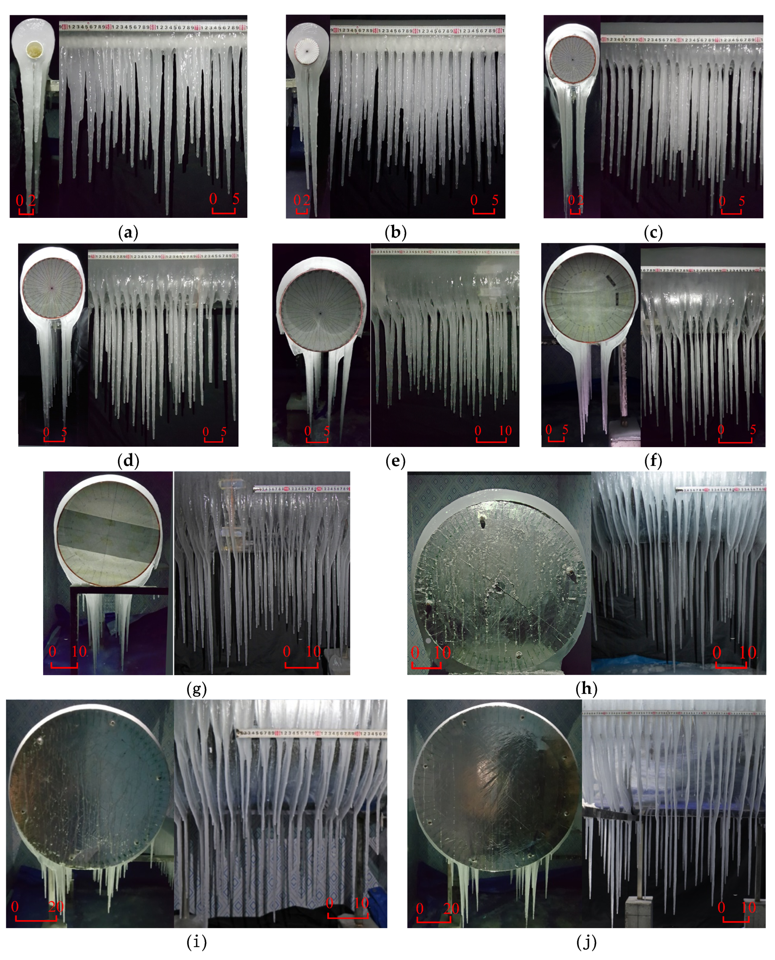
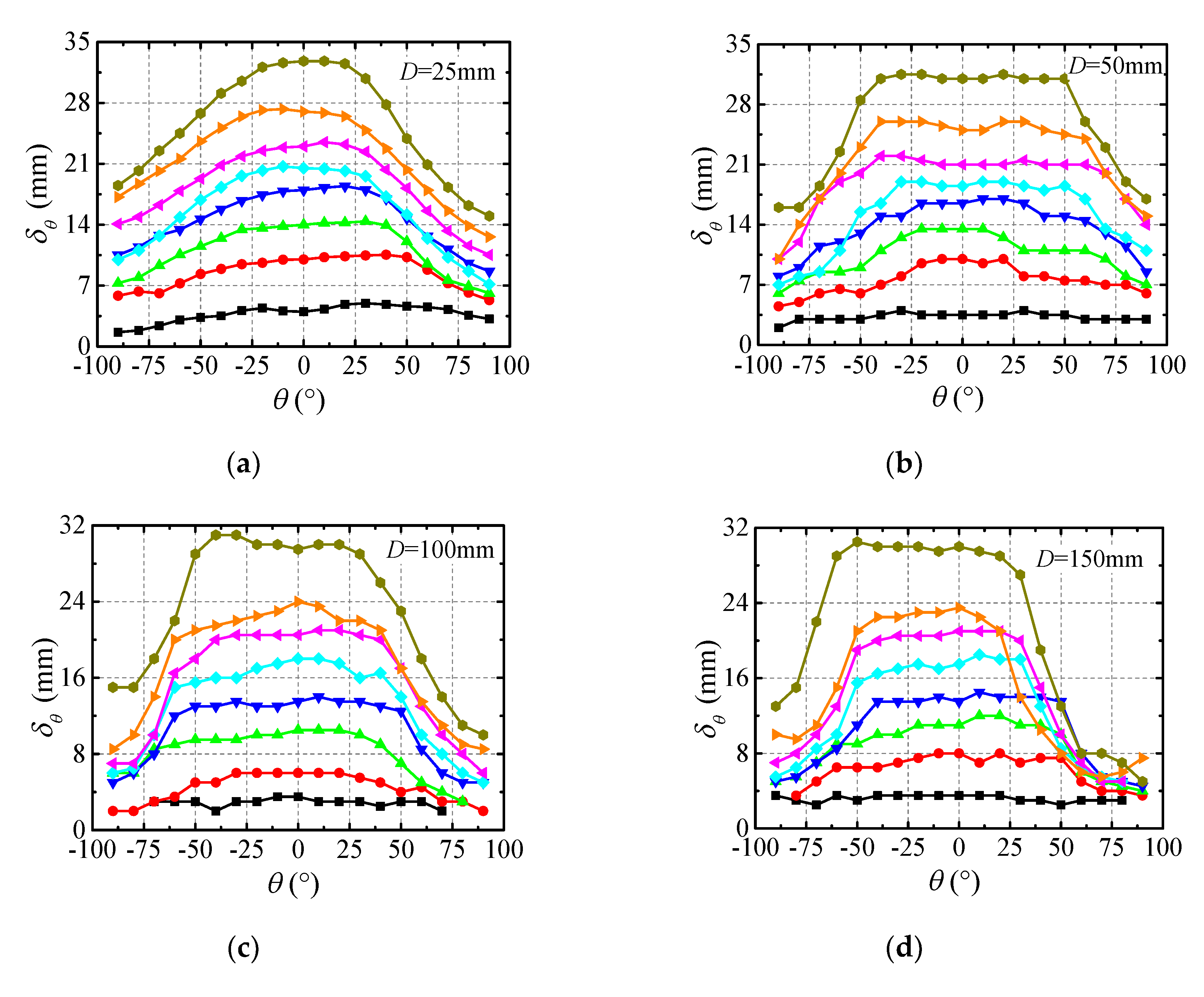
3.1.1. Influence of Pipeline Diameter

The profiles and side views of the ice accretion on pipelines with various diameters for N = 160 are shown in Figure 5. The droplets impinged smoothly upon the cylinder. Glaze ice accretion (smooth surface) was produced, and vertical icicles hung on both sides of the cylinder. The heat absorbed by the air was less than the latent heat produced due to the freezing of all the impinging droplets. Only a portion of droplets could freeze into radial ice on the pipeline surface, and the residual droplets then froze into icicles or were dragged away under the combined action of the aerodynamic force, gravity, and surface tension. The icicle hanging from the bottom of the cylinder was in accord with the results in Fukusako et al. [26] under small wind speed. However, icicles with an impact angle were produced in [16,41] since the runback water under the windy condition, and icicle hanging from the bottom of the cylinder tends to disappear gradually as the airstream velocity increased [26], the difference from previous results could be ascribe to the large wind speed. Pipelines with D ≤ 50 mm had no evident curved part, which was correspond with the icicle model on transmission lines [16,26,41]. For pipelines with D > 50 mm, the transverse width and length of the curved part increased with increasing D, while the longitudinal width was almost 5 mm. Consequently, the shape of the curved part resembled a sickle.
The radial ice sizes for pipelines with various diameters are shown in Figure 6. Figure 6a shows that the icing range of radial ice μ was non-uniform and decreased with increasing D. The radial ice thickness δ0 (Figure 6b) decreased with increasing D. δ0 and D approximately followed an exponential relationship: δ0 = a × Db. The values of δ0 were almost the same for the pipelines with various diameters in the early stage (e.g., N < 40 in the experiment), while δ0 increased in a similar manner with increasing N after the pipelines accreted a thin layer of ice. This suggested that the ice thickness differences mainly developed in the later stage (e.g., N ≥ 40 in the experiment). This can be explained as follows: (1) in the early stage, the area receiving droplets was proportional to the diameter, that is, to the amount of water contained along horizontal projected area of the cylinder, and consequently, the ice thicknesses for different D values developed at a similar speed; (2) at the later stage, the surfaces were covered by a thin layer of ice accretion, and the size effect of the ice accretion likely occurred because the Nusselt number depends on the Reynolds number, resulting that the heat transfer relates to D; (3) the collision efficiency of the droplets was smaller for large obstacles than for small ones. In summary, the ice sizes were closely related to the cylinder diameter, and the smaller diameter cylinder was more easily covered by ice.
For the present tests, the parameters l and s of icicles for different diameter cases were determined as shown in Figure 5 and Figure 7. There were remarkable non-uniformities of l and s. The non-uniformity of l was a consequence of the variations in s, which was due to the Rayleigh–Taylor instability [42] between two types of fluids (water and air) with different densities [15,43]. The spaces between the icicles were different, and the icicles received different quantities of droplets. For most cases, the mean icicle length lmean increased with increasing D, whereas it was opposite for the cases of D > 400 mm and N > 120. The growth rate of icicle length was controlled by the rate of heat loss from the surface to the environment. Longer icicles were the result of increases in the external heat flux combined with the availability of run-down water, which may be explained as follows: (1) the thermal convection of icicles is dependent on the Nusselt number, which increases with the Reynolds number, resulting that the icicle length increased with increasing D; (2) pipelines with larger D values had smaller curvatures, and hence required more kinetic energy to overcome the friction and aerodynamic force to drive the droplets to flow downward, therefore, the water flux to an icicle was reduced and led to an increased growth rate of the icicle length [44]; (3) unfortunately, there was insufficient space under the pipeline for icicle growth for the cases of D > 400 mm and N > 120. dt increased with increasing D. db almost remained constant (around 5 mm) which is in accord with the result in Maeno and Takahashi [45]. For D ≤ 400 mm, the mean longitudinal center-to-center spacing of icicle smean was insensitive to D and about 20 mm which was in accord with the result in Makkonen and Fujii [37]. For D > 400 mm, smean significantly larger than 20 mm which may be the influence of the surface material. The icicle may result in break-up if the adhesion strength (between the curved part and pipeline) was insufficient to support its weight, for example, a portion of the curved part would begin to separate from pipeline for the cases of D = 1000 mm after N = 220. Therefore, icicles cannot grow without limit.

3.1.2. Influence of Icing Duration

The ice profiles of typical pipelines are shown in Figure 8, Figure 9, Figure 10 and Figure 11, and the thickness δθ, icing range μ, and icicle length l for different cases are shown in Figure 12 and Figure 13.
The key observations and analyses can be summarized as follows:
(1)
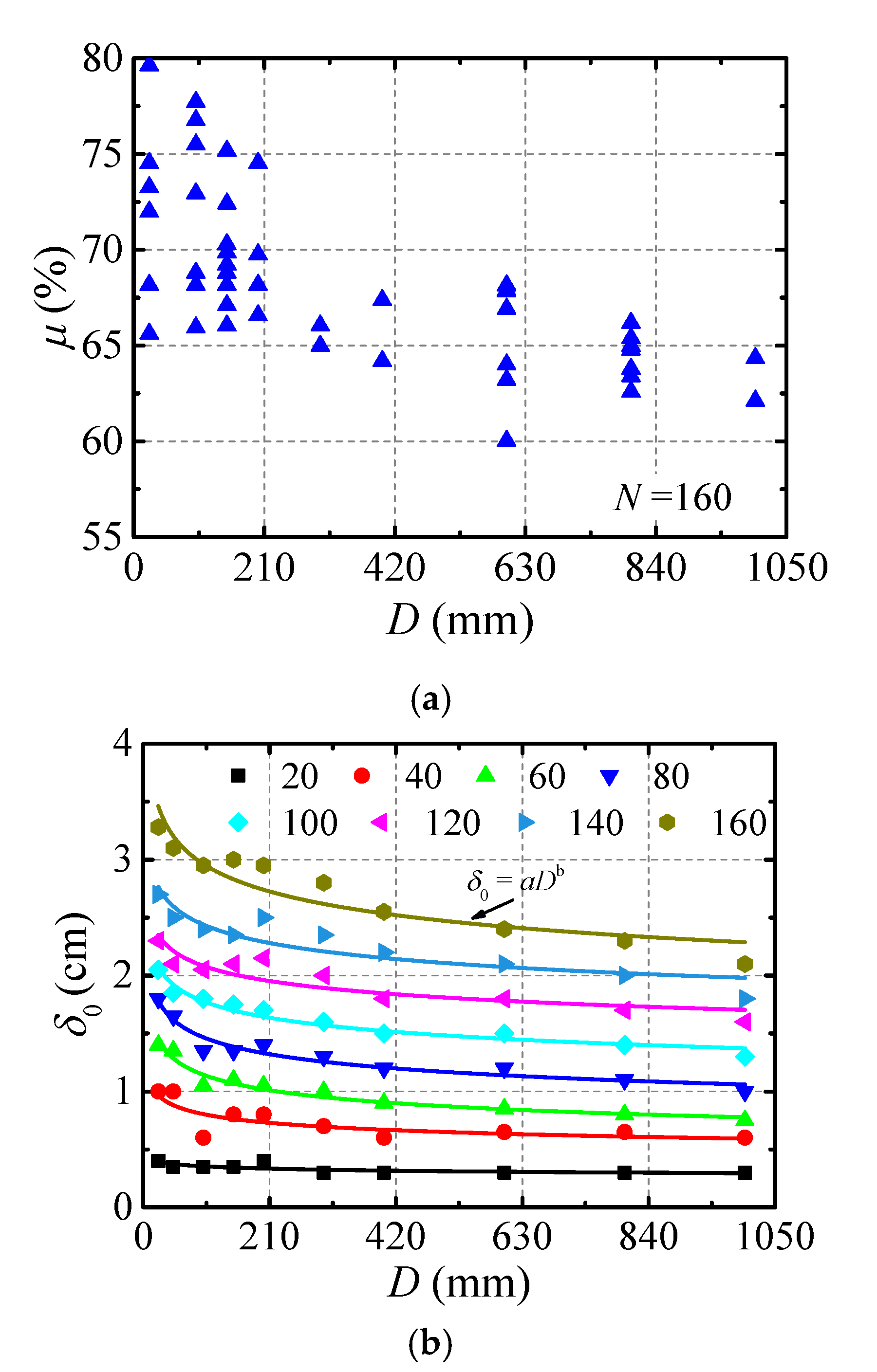
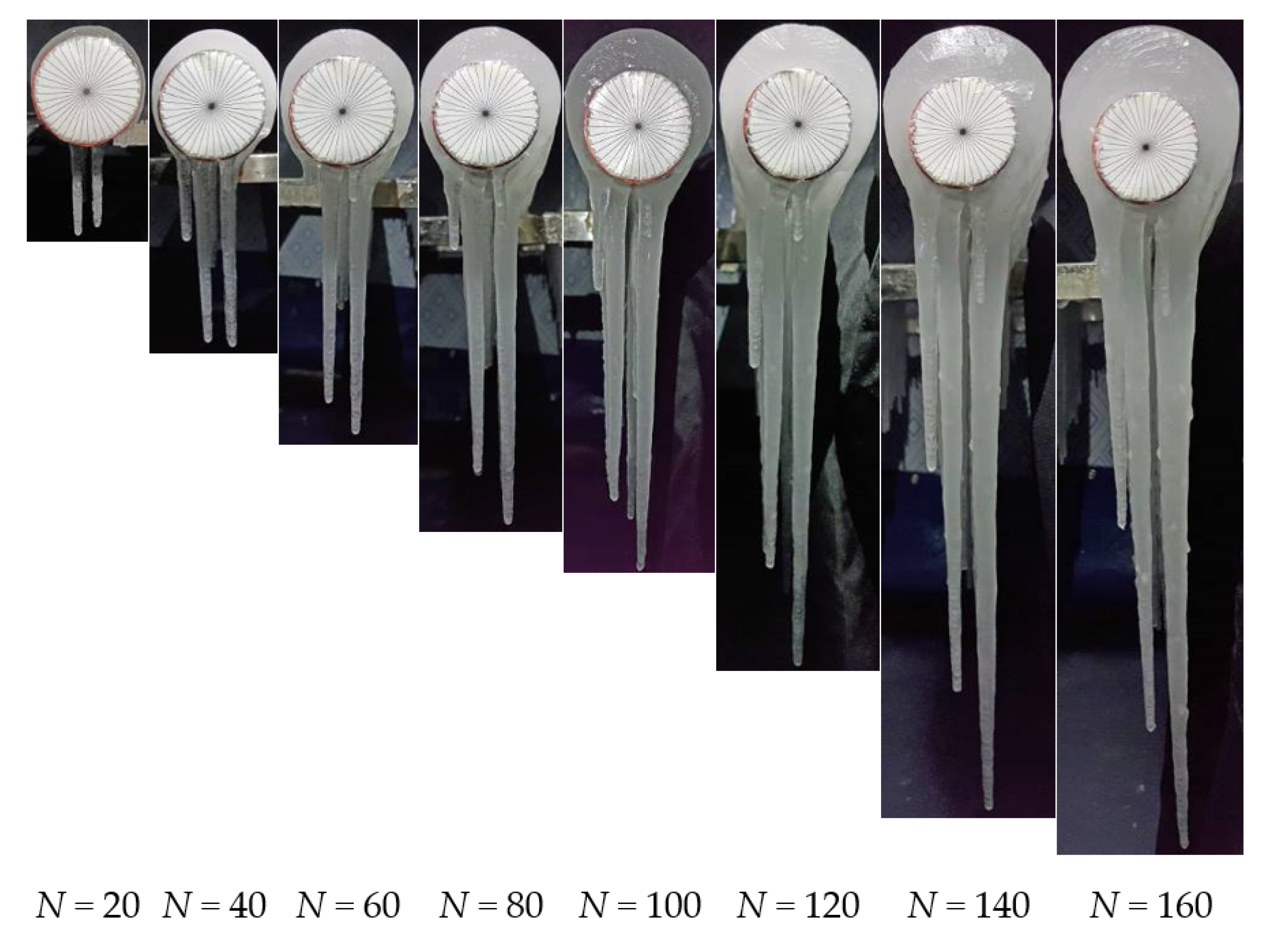
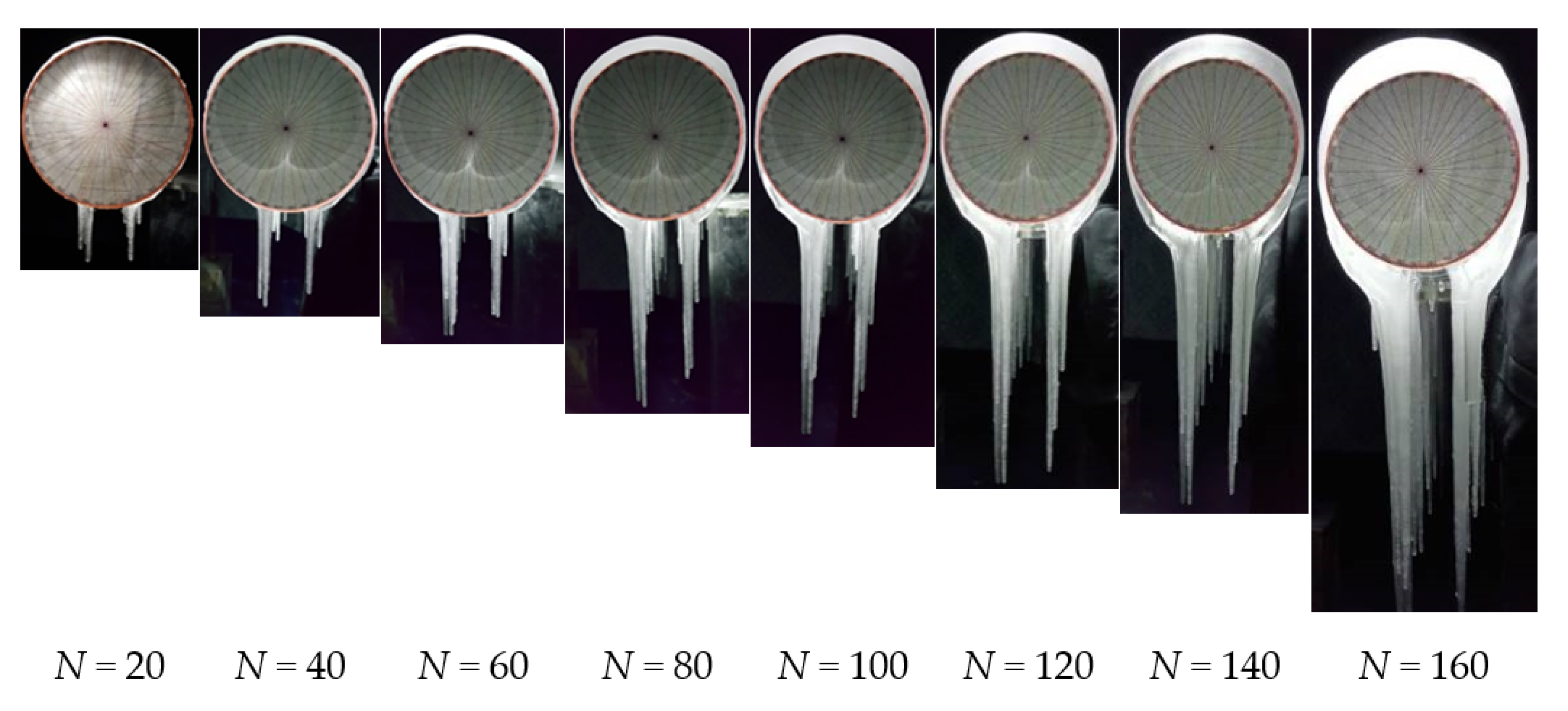
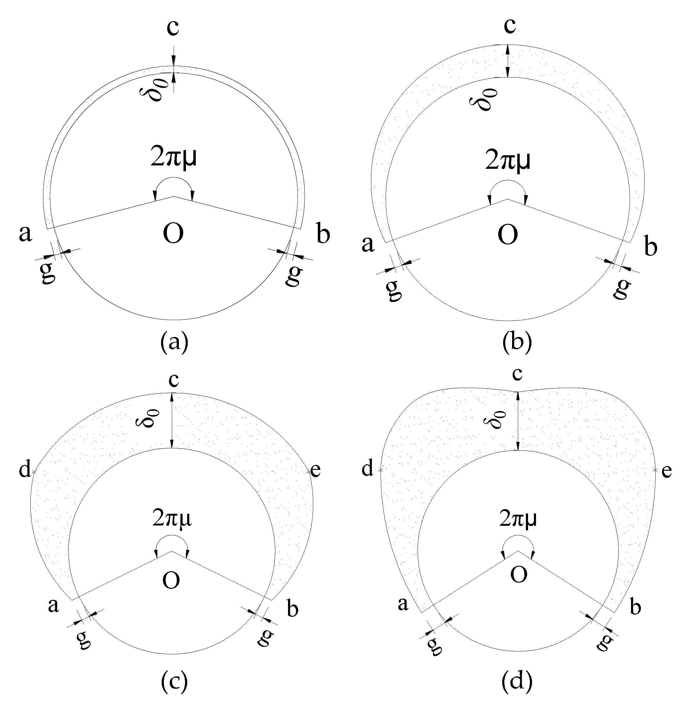
The ice profile changed with increasing N. A thin layer of annular-shaped ice formed at the early stage, the ice profile then changed from a crescent shape to a sector shape and finally to a D shape with increasing N, which can be simplified as the models shown in Figure 14. The annular-shaped ice had almost the same ice thickness at different positions. The crescent-shaped ice could be simplified as an arc, which could be characterized by several parameters: g (the thicknesses at the end point of the radial ice), δ0, and μ. The sector-shaped ice can be divided into three curved segments: ad, be, and dce, and the ice thicknesses at points d, c, and e were the same. The D-shaped ice could also be divided into three curved segments: ad, be, and dce, which had a smaller thickness at point c than that at points d and e. The annular-shaped ice was similar to the ice shape in Koss et al. [14] for high airstream velocities U = 30 m/s and T = −1 °C. The crescent-shaped and sector-shaped ice profiles were similar to those presented by Fukusako et al. [26] (U = 6 and 10 m/s, T = −15 °C) and Koss et al. [14] (U = 10 m/s and 20 m/s, T = −1 to −15 °C). The D-shaped ice was similar to the reverse-triangular ice presented by Fukusako et al. [26] for U = 10 and 20 m/s, T = −15 °C.
(2)
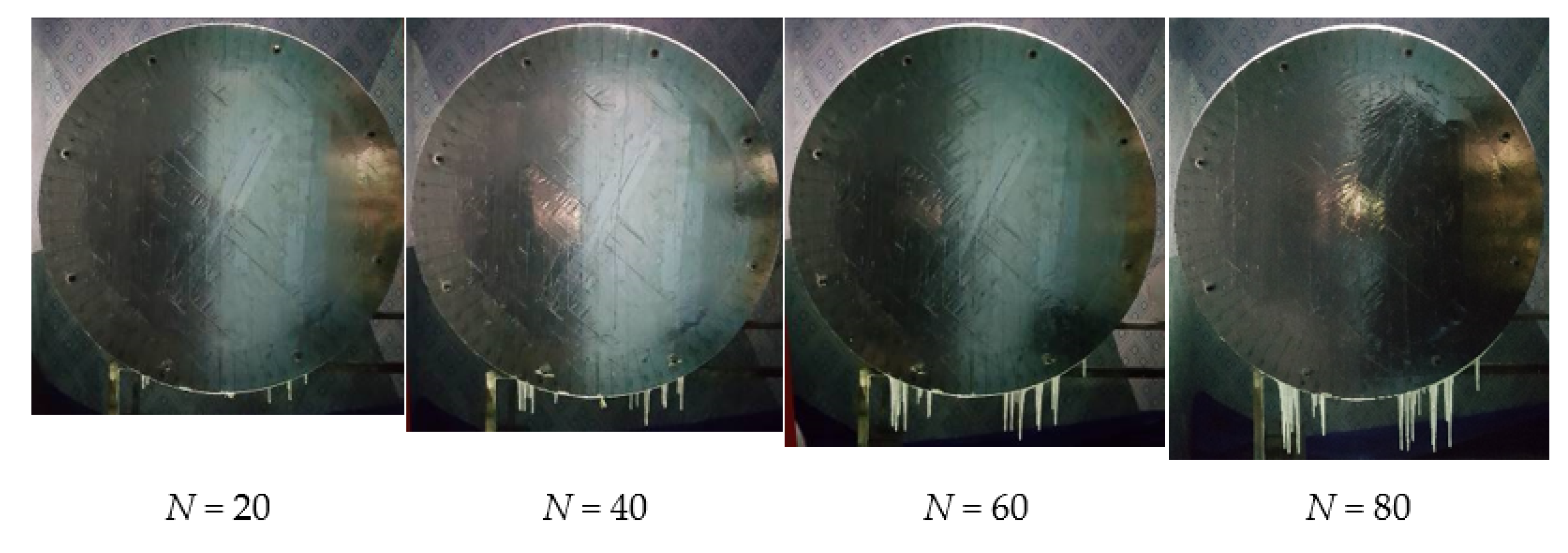
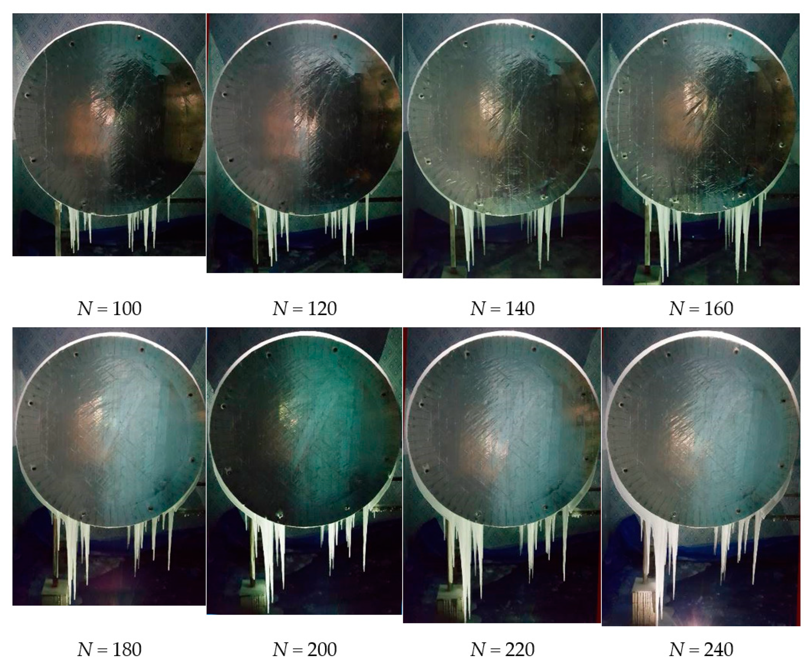
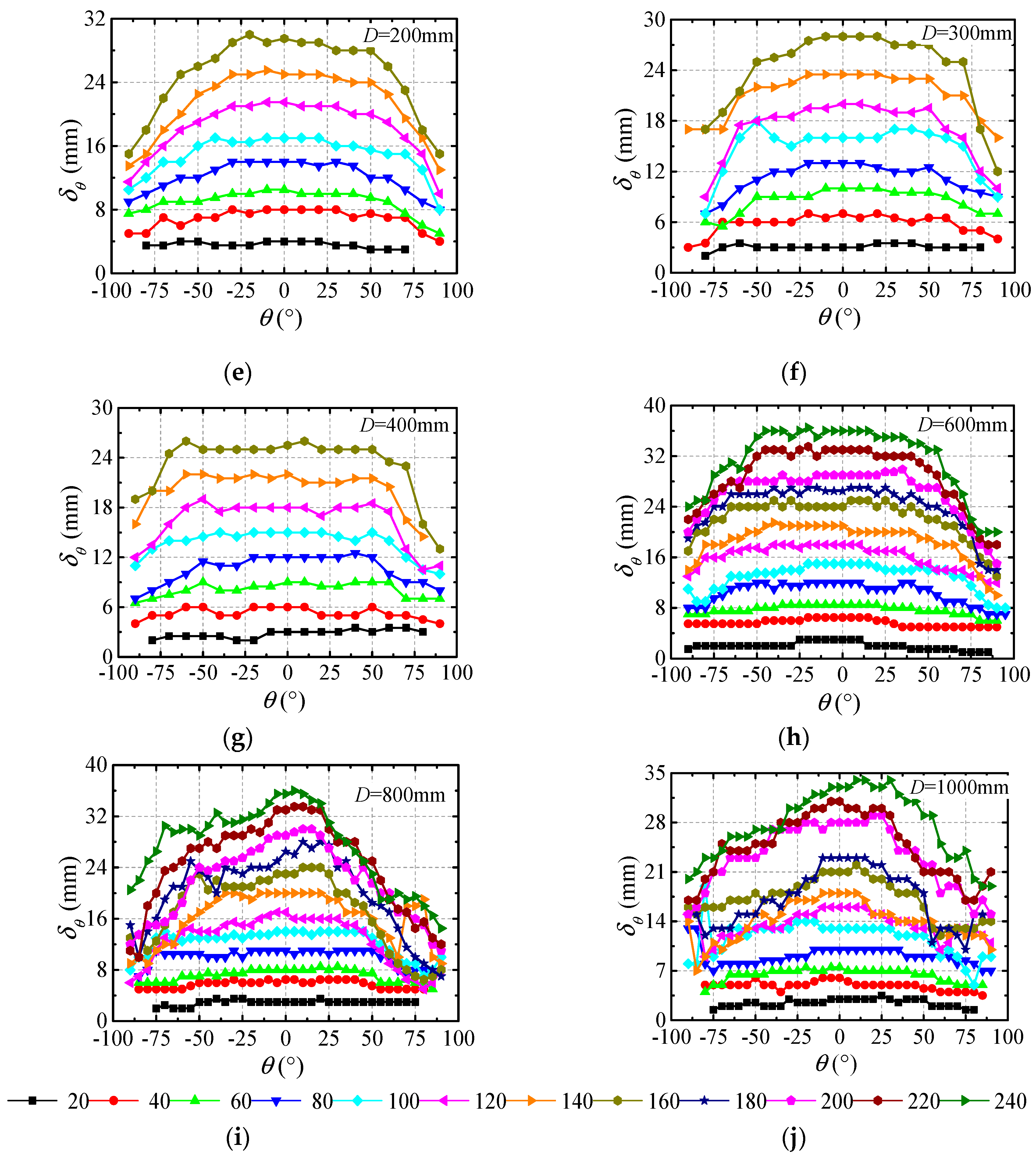
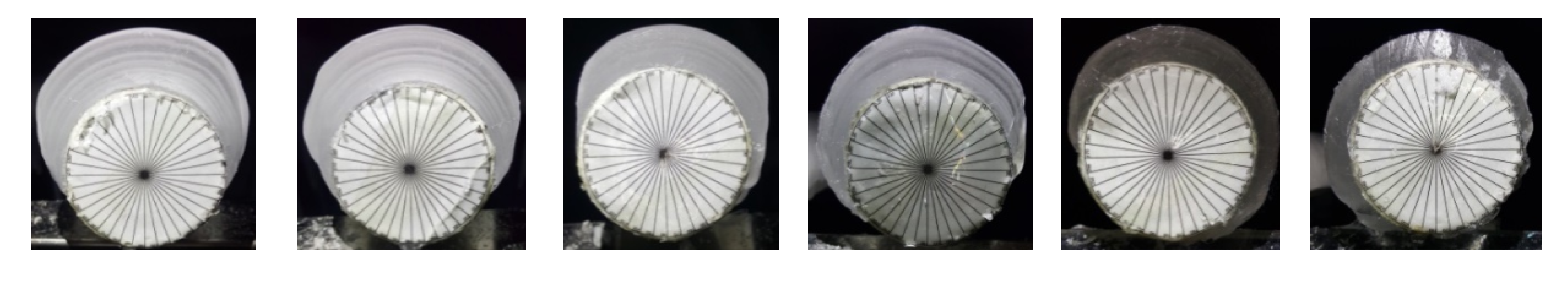
It is speculated that the larger diameter pipelines required longer times to form a specific type of radial ice under the same conditions. For example, for a pipeline with D = 25 mm (Figure 8), the ice profile was crescent shape when N = 20–40, and it became into sector shape when N = 60–160. For a pipeline with D = 150 mm (Figure 10), the ice profile was an annular shape when N = 20, and it became a crescent shape when N = 40 and 60, it became a sector shape when N = 80–140 and finally became D shape when N = 160. For a pipeline with D = 1000 mm (Figure 11), the ice profile was annular shape when N = 20–100, and it became crescent shape when N = 120–240.
(3)
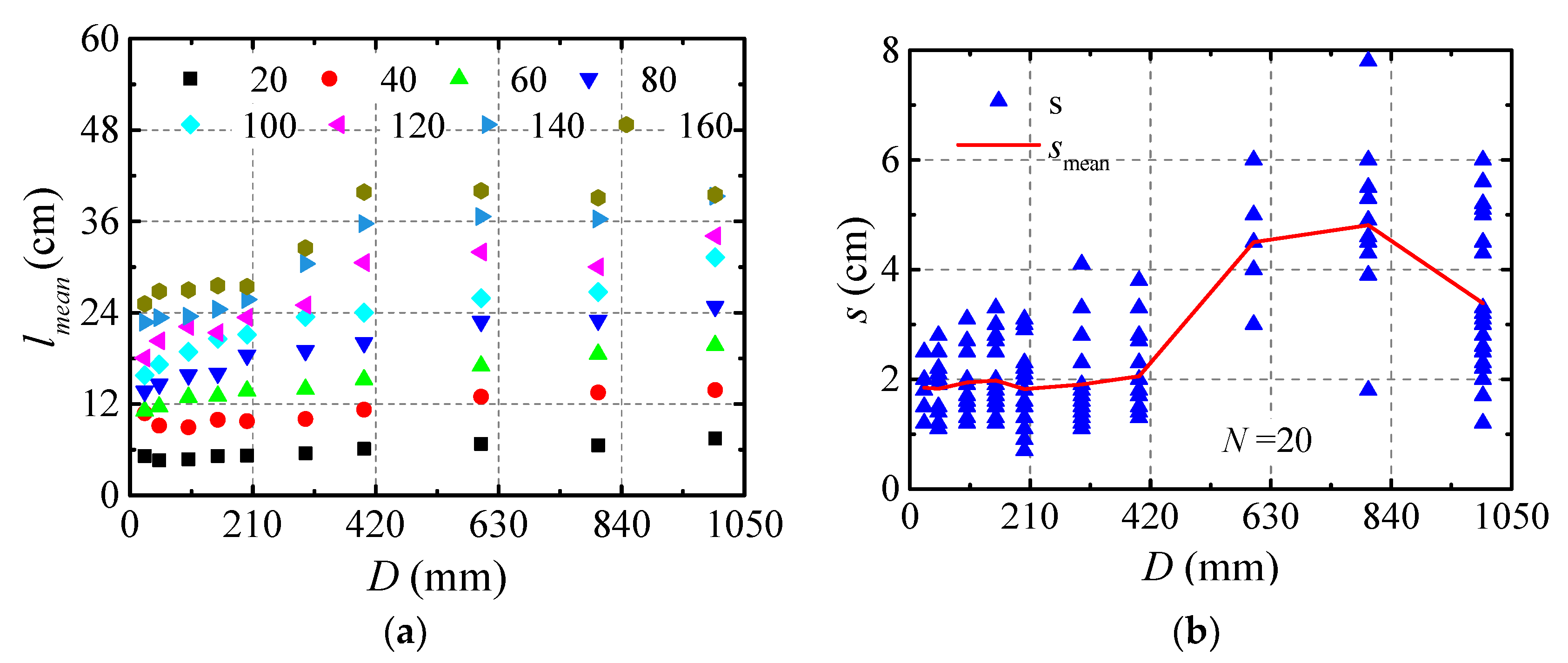
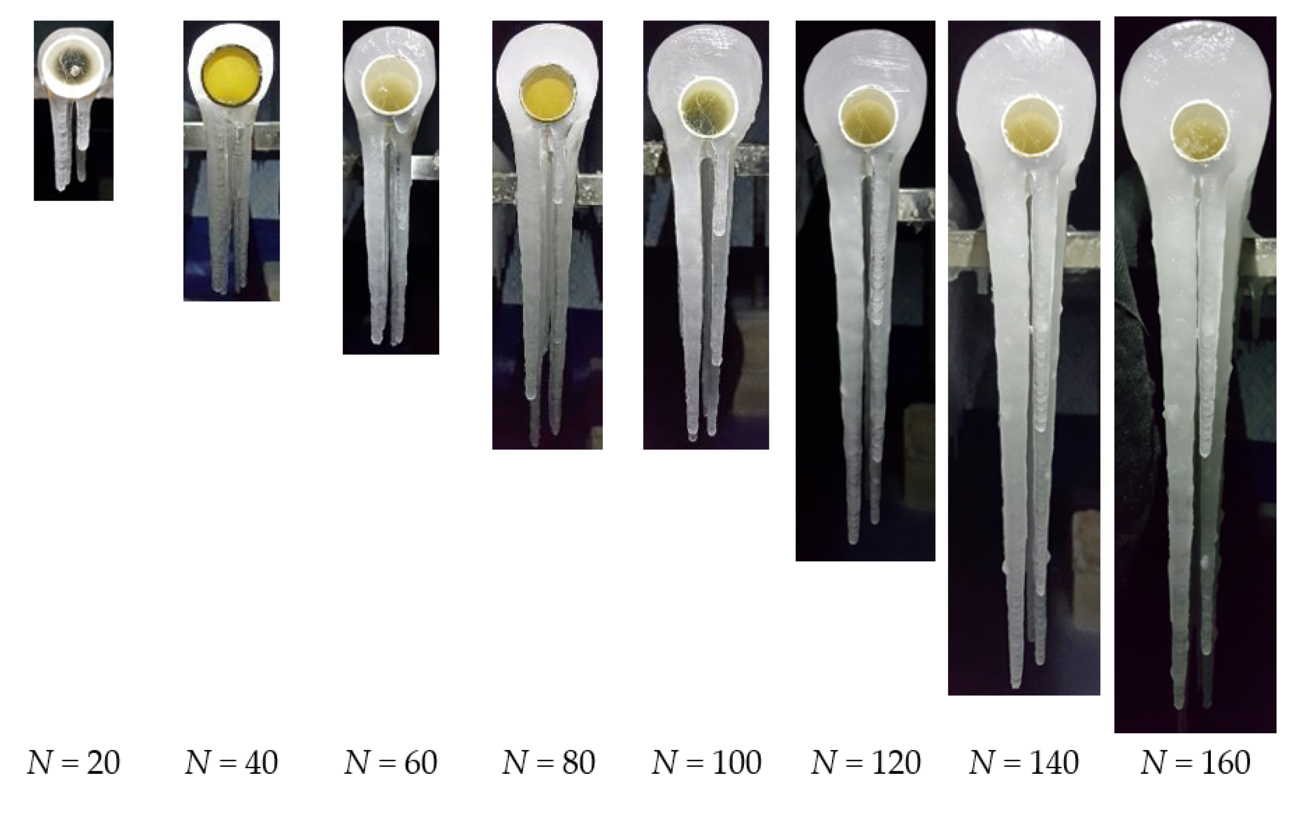
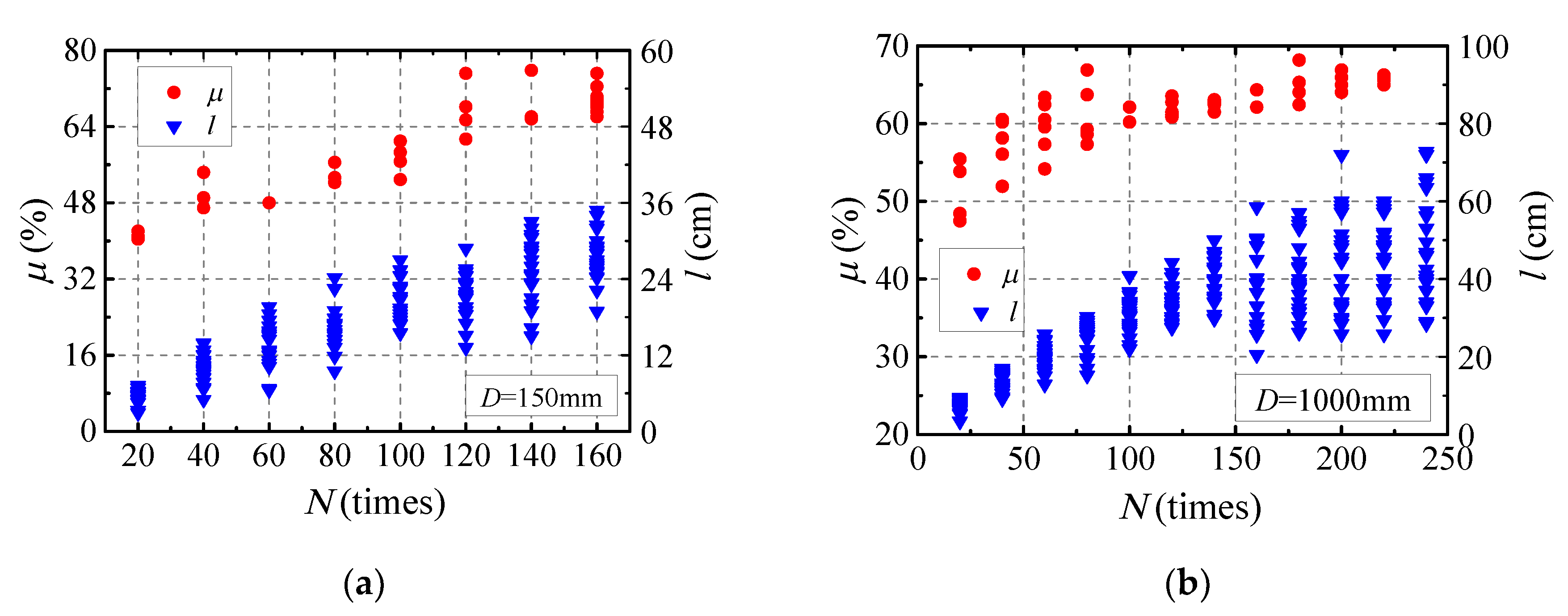
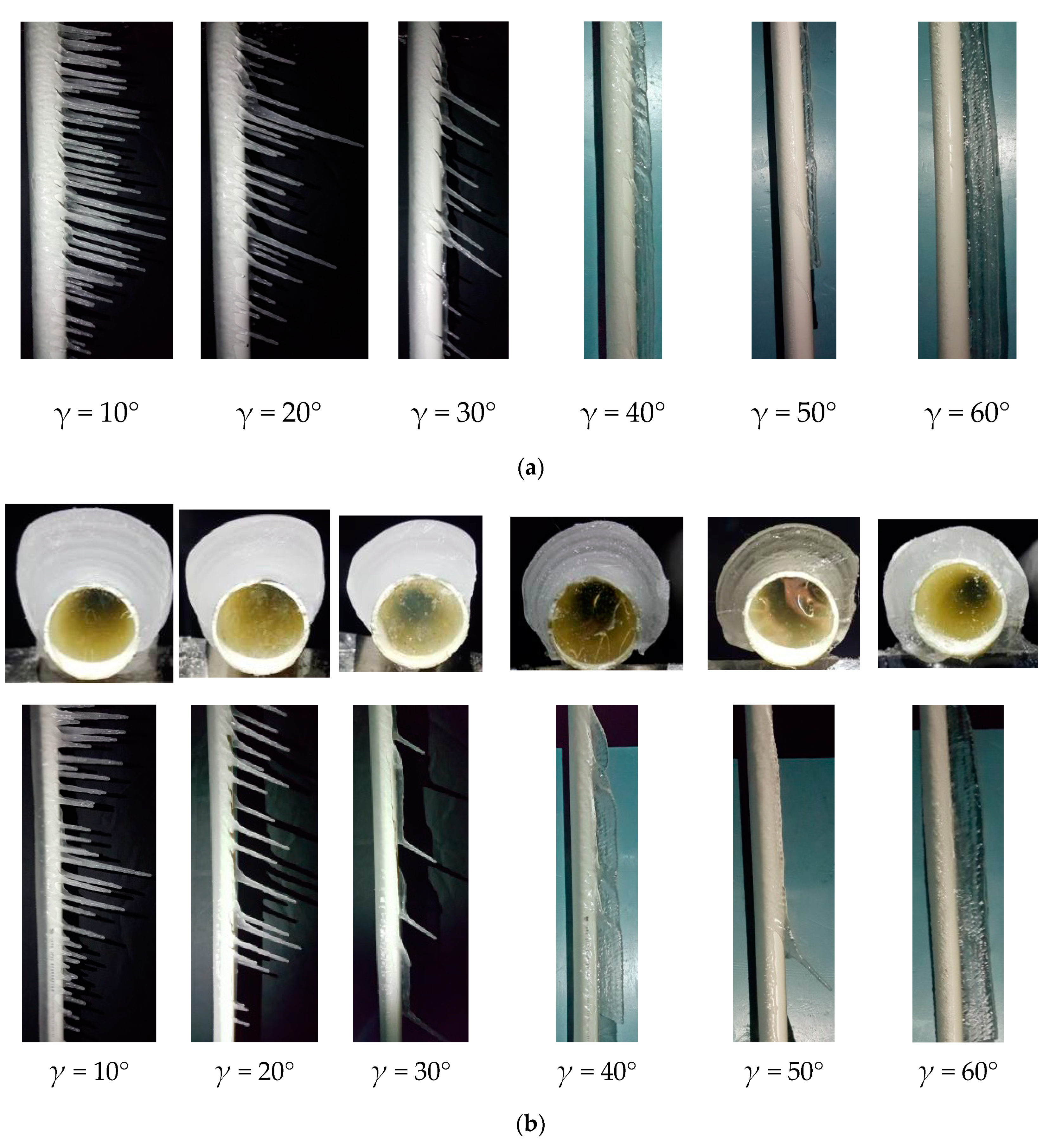
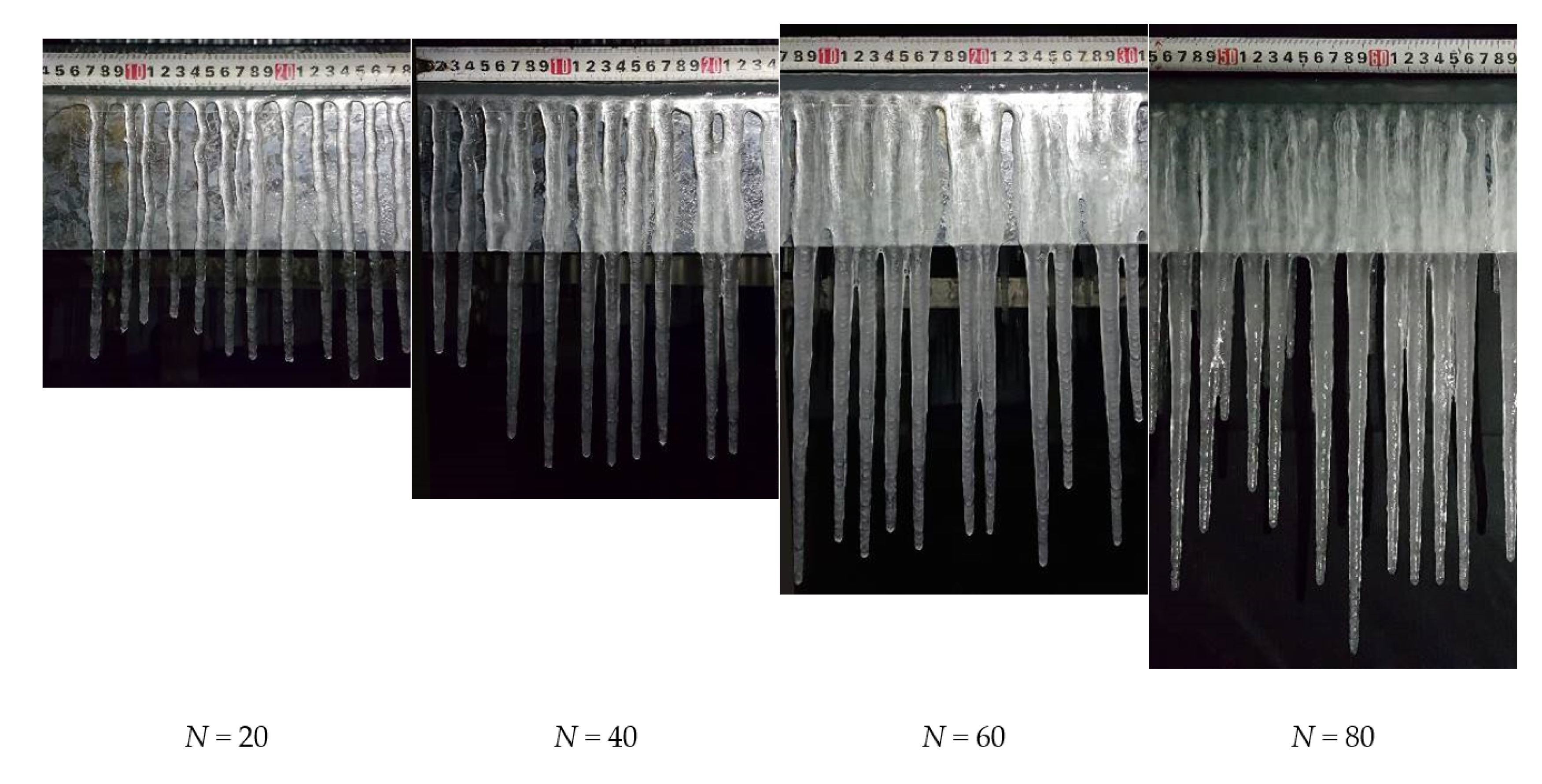
δ, μ, and l increased with increasing N (Figure 12 and Figure 13). The shape of the icicle changed with increasing N. For D = 150 mm (Figure 10), the top and bottom diameters of the linear part of the icicle were almost the same at N = 20, which could be simplified as a circular cylinder, it was similar to icicle shape presented by Fukusako et al. [26] (U = 6 m/s, T = −15 °C, 5 min elapsed); the top diameter then increased faster than the bottom diameter, and the linear part could be simplified as a circular truncated cone at N = 60, which was were similar to icicle shape presented by Fukusako et al. [26] (U = 6 m/s, T = −15 °C, 20 min elapsed); the linear part could be simplified as an elliptical cone since the transverse size of the icicle grew faster than the longitudinal size at N = 160. The curved part could be simplified as a sickle (Figure 15), whose longitudinal thickness was about 5 mm, and the transversal width increased with increasing N.

3.2. Ice Accretion on Wind Hanger

Kollár and Farzaneh [13] concluded that the ice mass accreted on a cylinder (D = 38 mm) decreased with increasing γ (γ = 61°–90°). The cylinders with D = 25–150 mm were taken as examples to investigate the influence of γ (γ = 0°–60°) on the ice shape and size on wind hangers. Figure 16 presents a series of photographs on the profiles and side views of ice deposits for D = 25 mm and 50 mm. The ice sizes are shown in Figure 17. In the lateral view, the separation point of the flow is well recognizable. The runback water flows mainly along the lower side of the wind hangers, giving rise to the formation of icicles or iced rivulets. Icicles are formed from the freezing of the water dripping or falling from wind hangers when γ = 0°–30°, while iced rivulets are produced due to the freezing of water flowing down along the wind hangers when γ > 30°. Iced rivulets were located around the flow separation line. The roughness of the radial ice increased with increasing γ. The thickness of the radial ice gradually decreased from the top to the bottom along the wind hangers, since the droplets were continuously captured and condensed into ice on the wind hangers when they flowed downward, and some of them could not flow to the bottom. The maximum δ0 decreased with increasing γ, which agrees well with the results of Kollár and Farzaneh [13]. That is ascribed to the fact that the amount of the downflow water along the wind hanger increases with increasing γ. And l also decreased with increasing γ. Because more droplets flowed down the wind hanger with increasing γ, and the less droplets can be captured by the icicles.

3.3. Ice Accretion on Section Steel

The ice shapes of the medium-size section steels at various γ are shown in Figure 18, and the side views of ice accretion for L100 and γ = 90° at different N are shown in Figure 19. The mean ice sizes of the section steel at N = 80 are listed in Table 2.
The key observations are summarized as follows:
(1)
Figure 18 shows that two rows of icicles formed on the two sides for each section steel, and ice was produced on the surfaces facing the droplets. The icicle length and spacing had significant non-uniformity. The size effects of Bt, Bb, and Bs were non-significant, as shown in Table 2.
(2)
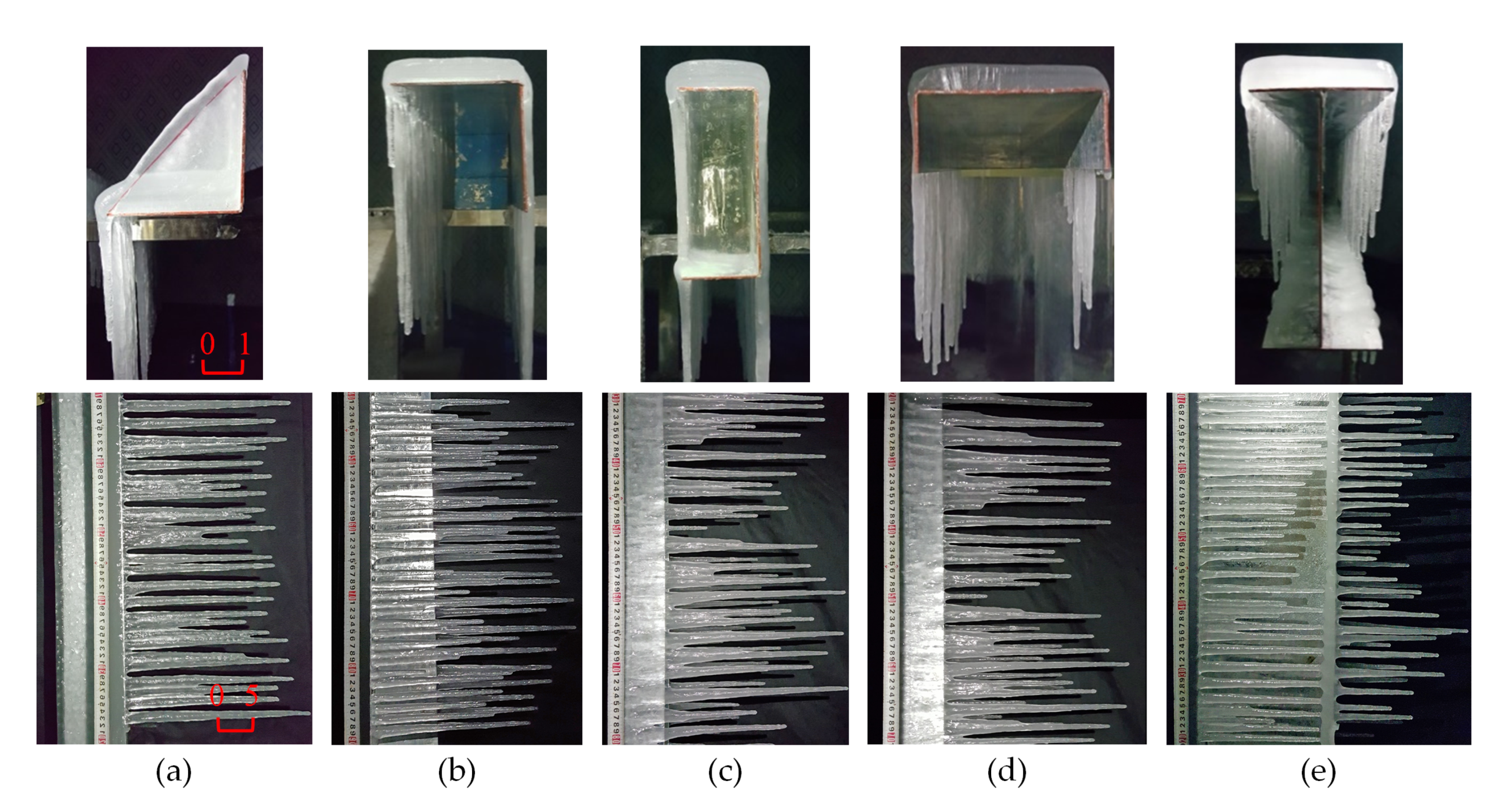
For the angle steel, the ice thickness on the top wall (γ = 90°) was smaller than that on the bottom wall (γ = 0°). This was due to some of the droplets being prevented from flowing down by the lateral wall for γ = 0°, and consequently, Bb > Bt. ls for γ = 0° was much larger than that for γ = 90°. For the U-steel and I beams with γ = 0°, most of the icicles were connected to the bottom wall, and therefore, the lt values in Table 2 were inaccurate.
(3)
As shown in Figure 18 and Figure 19, the icicles on all components could be simplified as circular truncated cones with s = 2–52 mm. The db of the icicle was about 5 mm, while dt increased with increasing N, and the adjacent icicles would connect after dt > s, therefore the individual icicles begin to merge into an icicle curtain. At the early stage, ice on the lateral wall was in the form of flat icicles, and only some local areas accreted ice. The whole range was almost uniformly covered by ice when N was large enough.

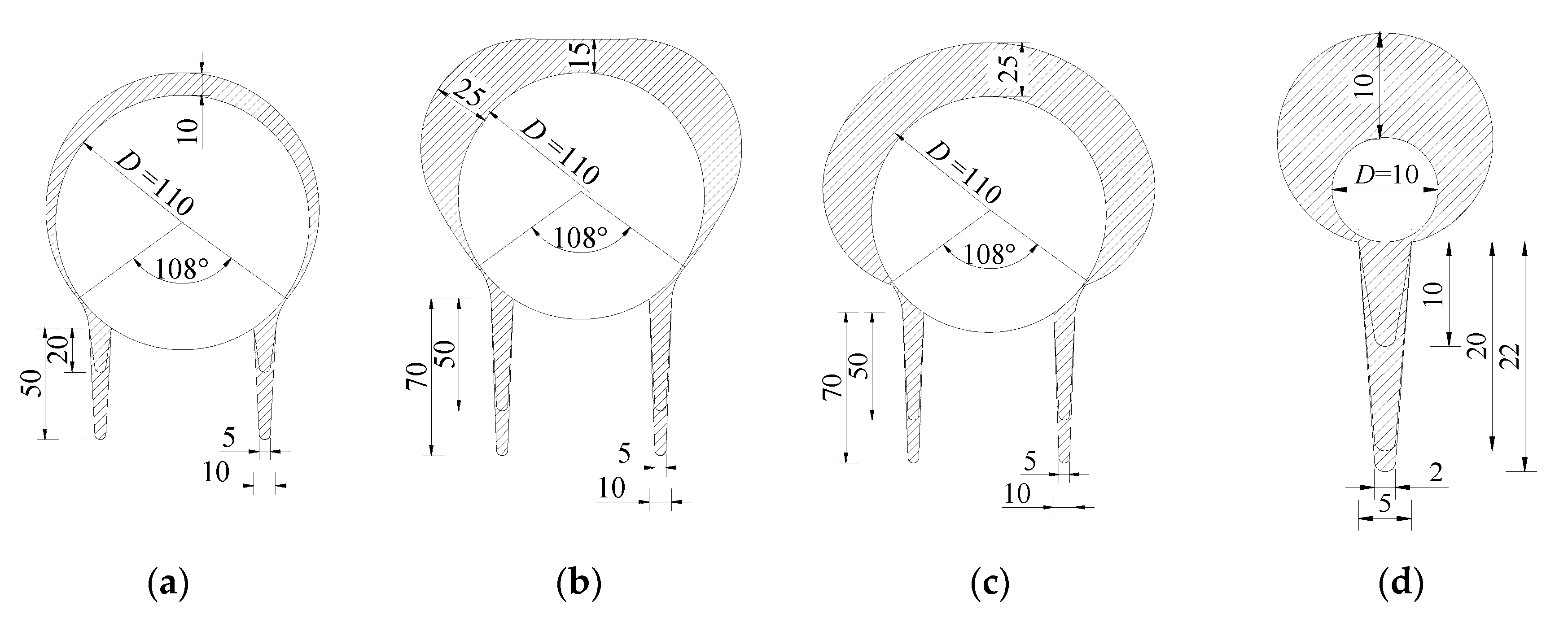
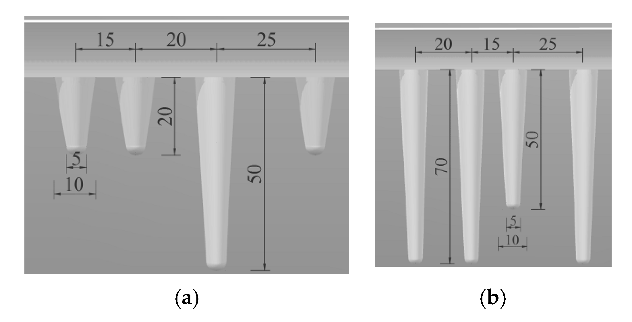
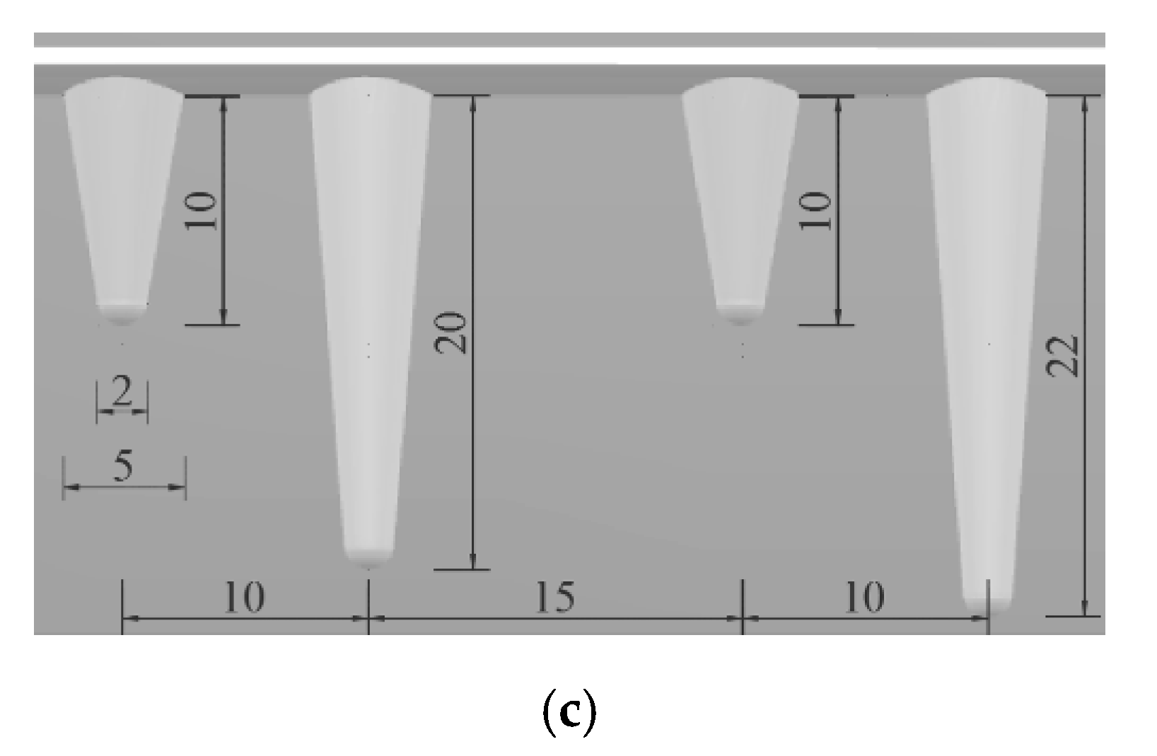
3.4. Ice Accretion on Sectional Model

The ice accretions on sectional models of girders A, B, and C (N = 30) are shown in Figure 20, and the details of the grate plate for girders A and B are shown in Figure 21.
The major observations are summarized as follows:
(1)
The ice thicknesses and ice shapes on the pipelines of the section models were roughly the same as those on the circular cylinders described in Section 3.1. Only one row of icicles was formed under each guardrail of girders A and B due to its small diameter (D = 10 mm), which agreed with the results for ice accretion on transmission lines [37].
(2)
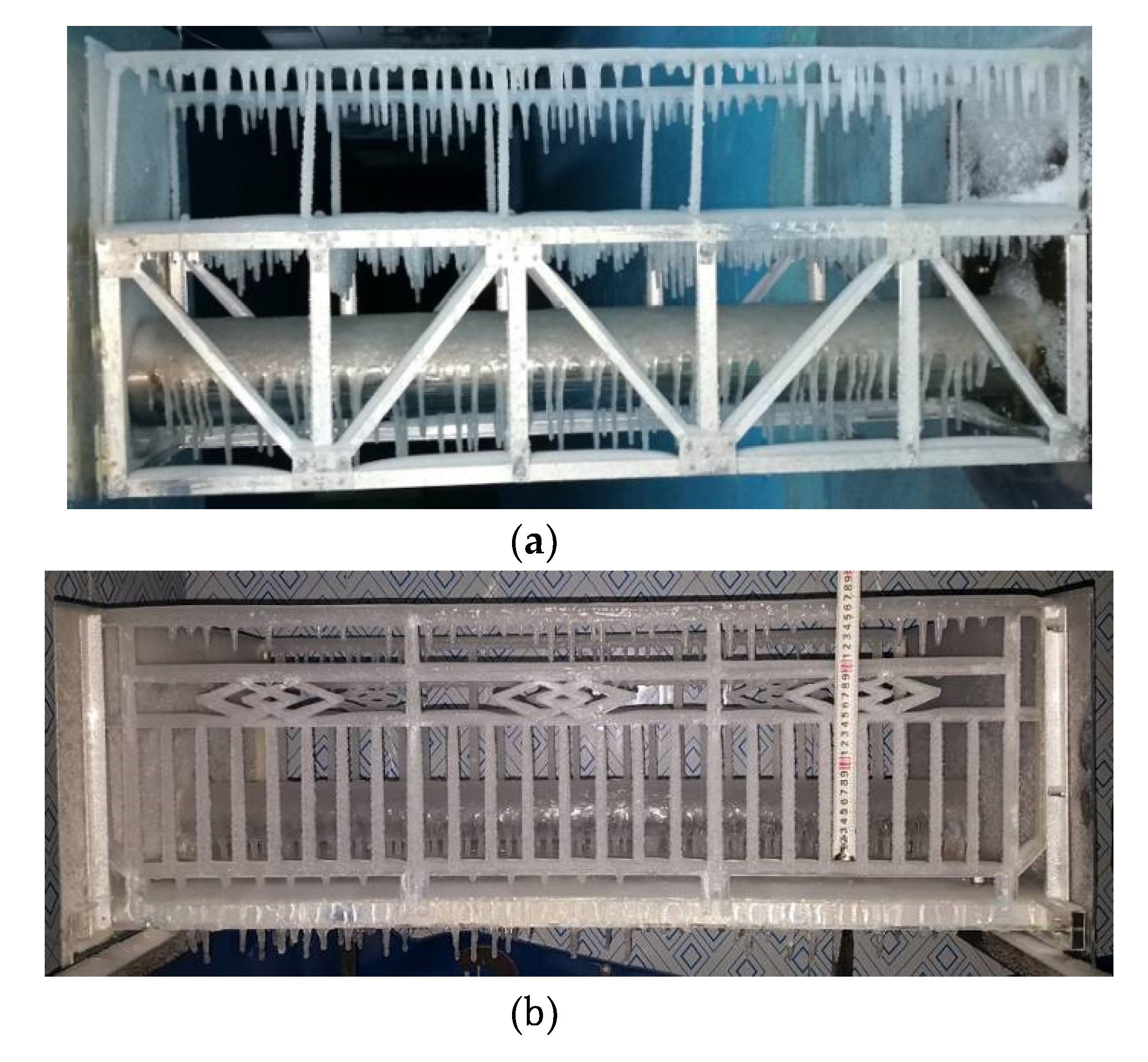
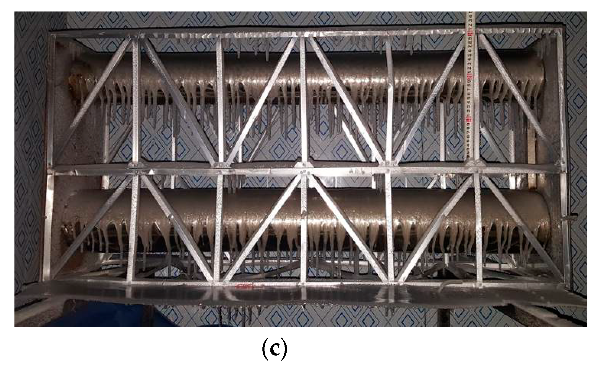
The ice shape of the truss stiffening girder was related to the γ of its components. A large amount of ice accumulated on the upper surface for the horizontal and inclined bars, while only a slight amount of ice with a rough surface grew on the surfaces of the vertical bars, and the other surface of the truss stiffening girder had little ice. The areas and thicknesses of the components facing the droplets were increased by the ice on the truss stiffening girder. These results agreed with those in Section 3.3. Therefore, the above results for pipelines and section steels could be used as references for simulating the ice accretion on pipeline girders.
(3)
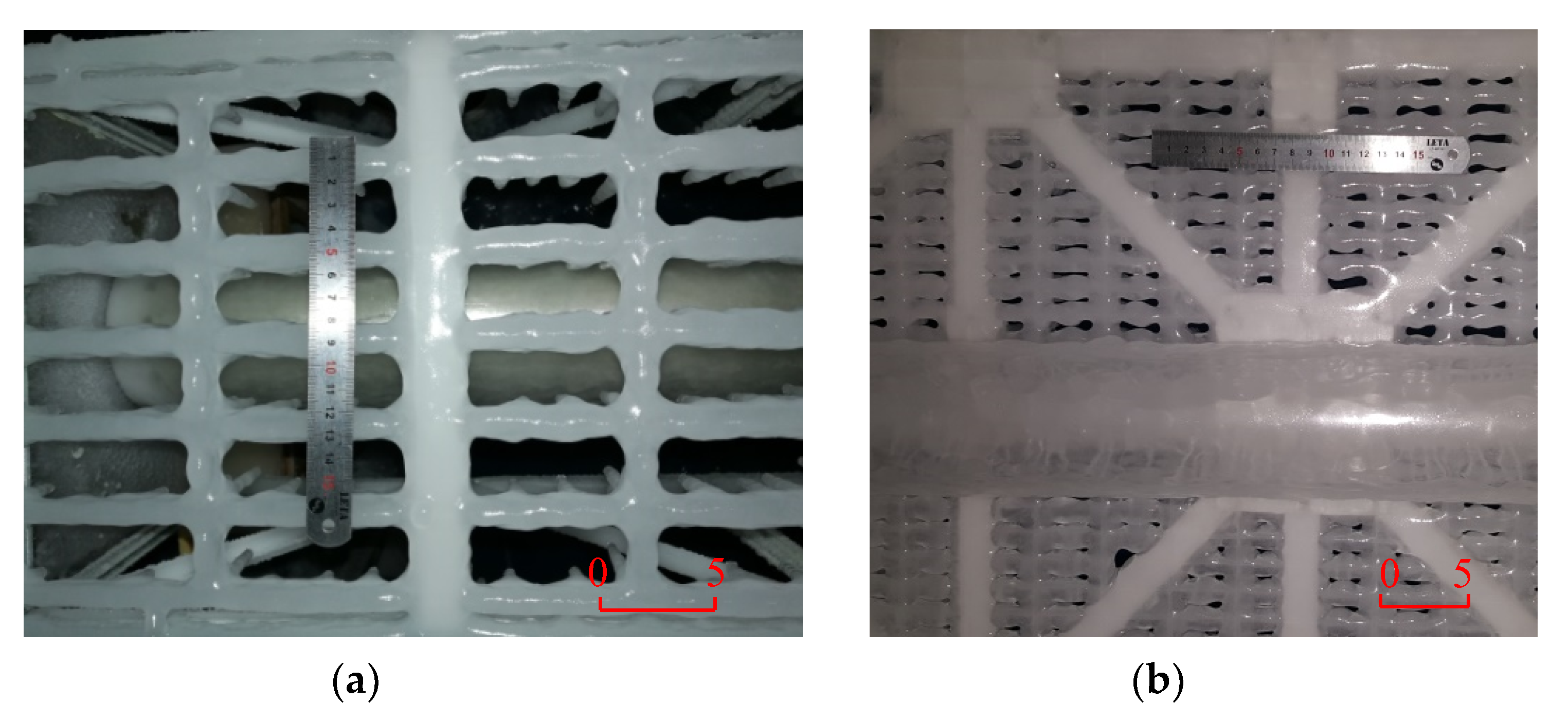
Since the grate plate was composed of interconnected slender elements, the ice accretion on adjacent elements connected, which resulted in a decreased porosity and an increased thickness, respectively (Figure 21). Meanwhile, a large number of icicles were produced under the grate plate, which was like a large icicle matrix. However, the sizes of the icicles under the grate plate had upper limit, and they would stop growing after the porosity of the grate plate became zero.
(4)
For girder C, due to the obstruction of the upper pipeline and truss, the δ0 of the upper layer (5 mm) was much larger than that of the lower layer (2 mm), and the lmean of the upper pipeline (85 mm) was larger than that of the lower pipeline (59 mm). Bt of the middle horizontal trusses (13.6 mm) was larger than that of the top ones (10.5 mm), while the average Bt of the bottom section steel was the smallest one (7.7 mm).

4. Shape Simulation of Ice Accretion on Sectional Model

The experimental results in Section 3 can provide references for shape simulation of ice accretions on pipeline suspension bridges. To investigate the influence of ice accretion on the aerodynamic characteristics of pipeline suspension girder with girder A, three types of radial ice (the crescent-shaped, D-shaped, and sector-shaped ice accretion) and two length of icicles on the pipeline were selected referencing experimental results in the Section 3.1 and Section 3.4. Circular truncated cone shaped icicles were selected. Under some external factors (e.g., aerodynamic interference, wind speed, and freeze-thaw), the D-shaped ice might be prior to the sector-shaped ice. Thickness of crescent-shaped radial ice was smaller than that of the other radial ice, therefore icicles with crescent-shaped radial ice were shorter than those with the other radial ice. Combining the above reasons, the corresponding ice shapes on pipeline are shown in Figure 22 and Figure 23. The large ice thicknesses at the top of the three radial ice were designed to simulate the extreme condition. The ice accretion on angle steel and U-steel were simulated by adhesive tapes with a width of 20 mm and thickness of 3 mm, which were glued onto the surfaces that were facing droplets. A plexiglass plate with a larger thickness (10 mm) and smaller porosity (64%) was used to simulate the icing grate plate. Crescent-shaped ice was applied to simulate the radial ice of a guardrail (Figure 22d), while dt and db were 5 and 2 mm, respectively, and the icicle spacing is shown in Figure 23c. The ice accretion models of the pipelines and guardrails were printed by 3D printing technology and then glued on the sectional model. The surface of the artificial ice was smooth, and the effect of roughness of ice accretion was not considered.
Icing of a pipeline suspension girder is a very complicated process. Wet growth (with icicle) and dry growth (without icicle) may occur under low-temperature conditions [46]. To investigate the influence of the above process and ice accretion on various components, five ice classes C0 (ice-free), C1 (pipeline with radial ice), C2 (C1 + pipeline with icicle), C3 (C2 + guardrail with ice), and C4 (C3 + truss stiffening girder and grate plate with ice) were studied. In addition, the influence of the ice accretion types (Figure 22 and Figure 23) on the aerodynamic force coefficients was also comprehensively investigated.

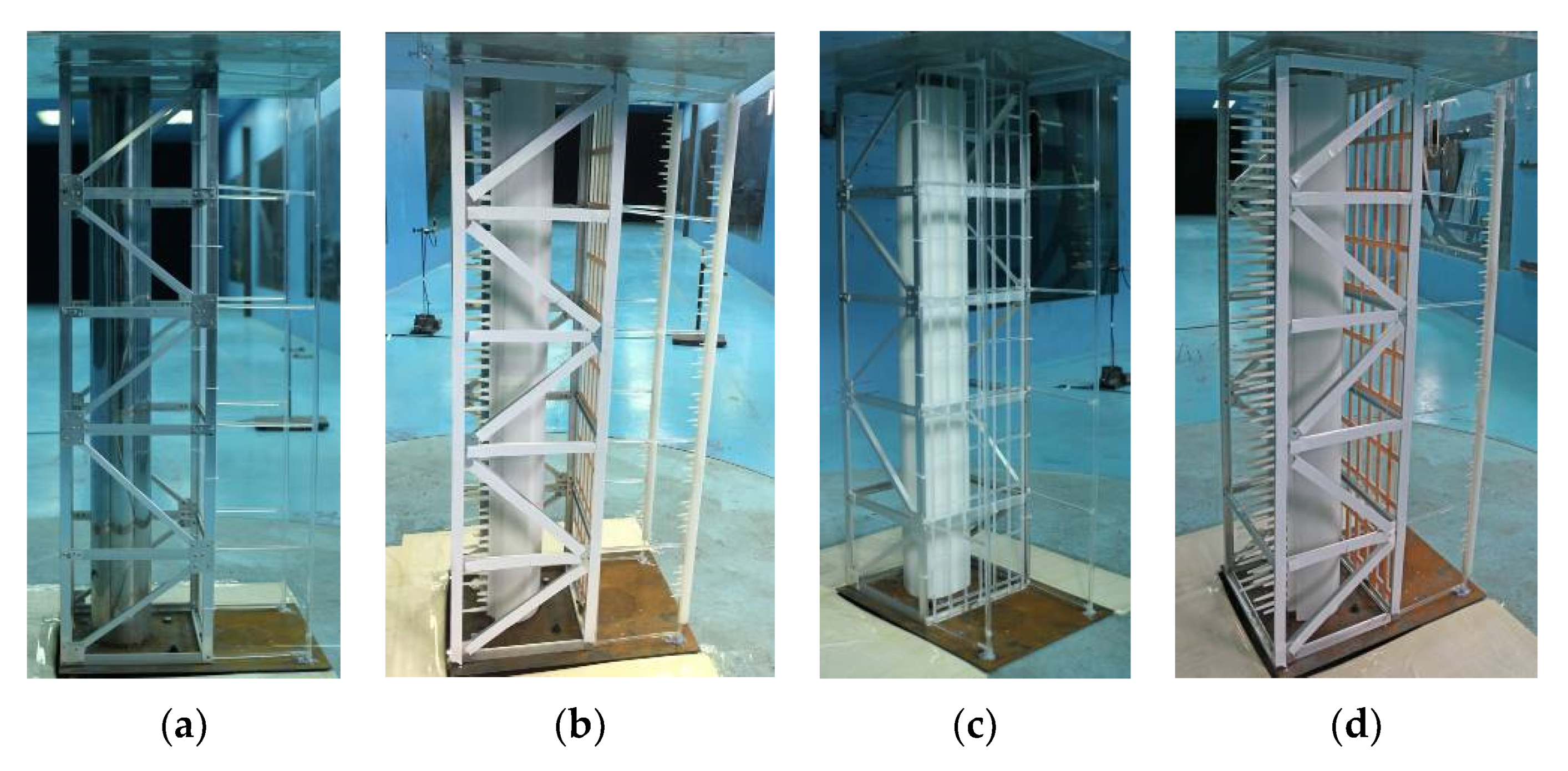
5. Wind Tunnel Tests

5.1. Experimental Setup

The experiments were carried out in the DUT-1 boundary layer wind tunnel of the Dalian University of Technology in China. The closed-circuit wind tunnel had a work section with dimensions of 18.0 m (length), 3.0 m (width), and 2.5 m (height). The wind velocity could be adjusted continuously between 1 and 40 m/s. All of the tests were carried out in smooth flow with a turbulence intensity below 1%.
The aerodynamic force coefficients CD(α), CL(α), and CM(α) of sectional model A were investigated, where is the angle of attack. With reference to Figure 3a, for drag force (FD(α)), lift force (FL(α)), and pitching moment (M(α)) of the girder, CD(α), CL(α), and CM(α) are defined as follows:
C D ( α ) = F D ( α ) 0.5 ρ U 2 H L
C L ( α ) = F L ( α ) 0.5 ρ U 2 B L
C M ( α ) = M Z ( α ) 0.5 ρ U 2 B 2 L
where U is the wind speed (15.5 m/s), L = 1030 mm, B = 324 mm, H = 417 mm, and ρ is the air density.
As shown in Figure 24, the model was fixed to a six-direction-component high-frequency balance (under the steel plate in Figure 24) by four screws, and the point O in Figure 3a was located at the center of the screws. The measurement ranges of the three forces were 0–300, 0–300, and 0–600 N, respectively, and the ranges of the bending and torsional moments were 0–57 N·m, with a relative precision of 0.06% of the full-scale. A thin steel plate with 1.2 m width and 1.2 m length was placed on the top end of the model to ensure nominally two-dimensional flow. The acquisition time was 30 s, and the data-sampling frequency was 100 Hz. α varied in the range of −12° to 12° with an increment of 1°.

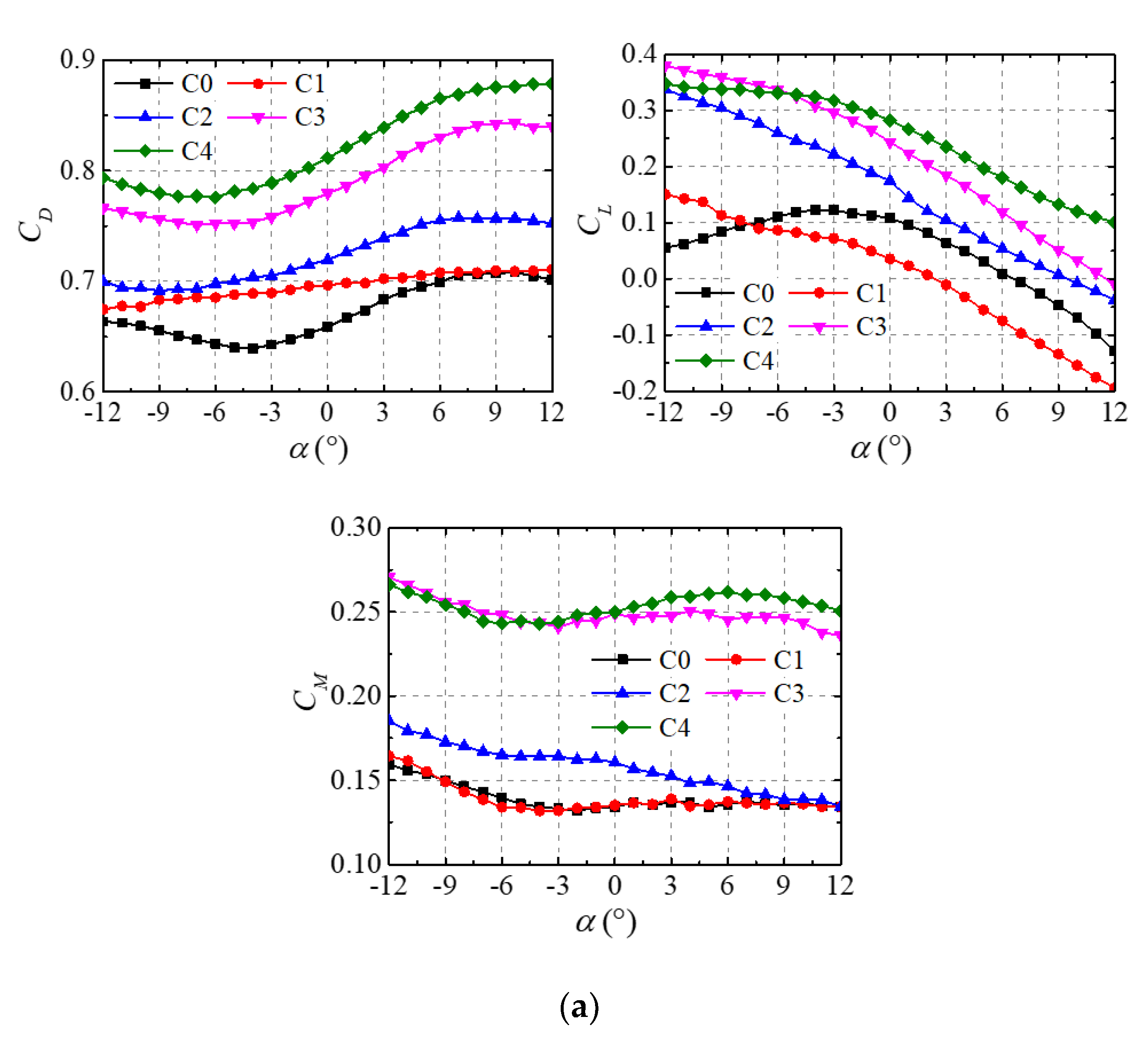
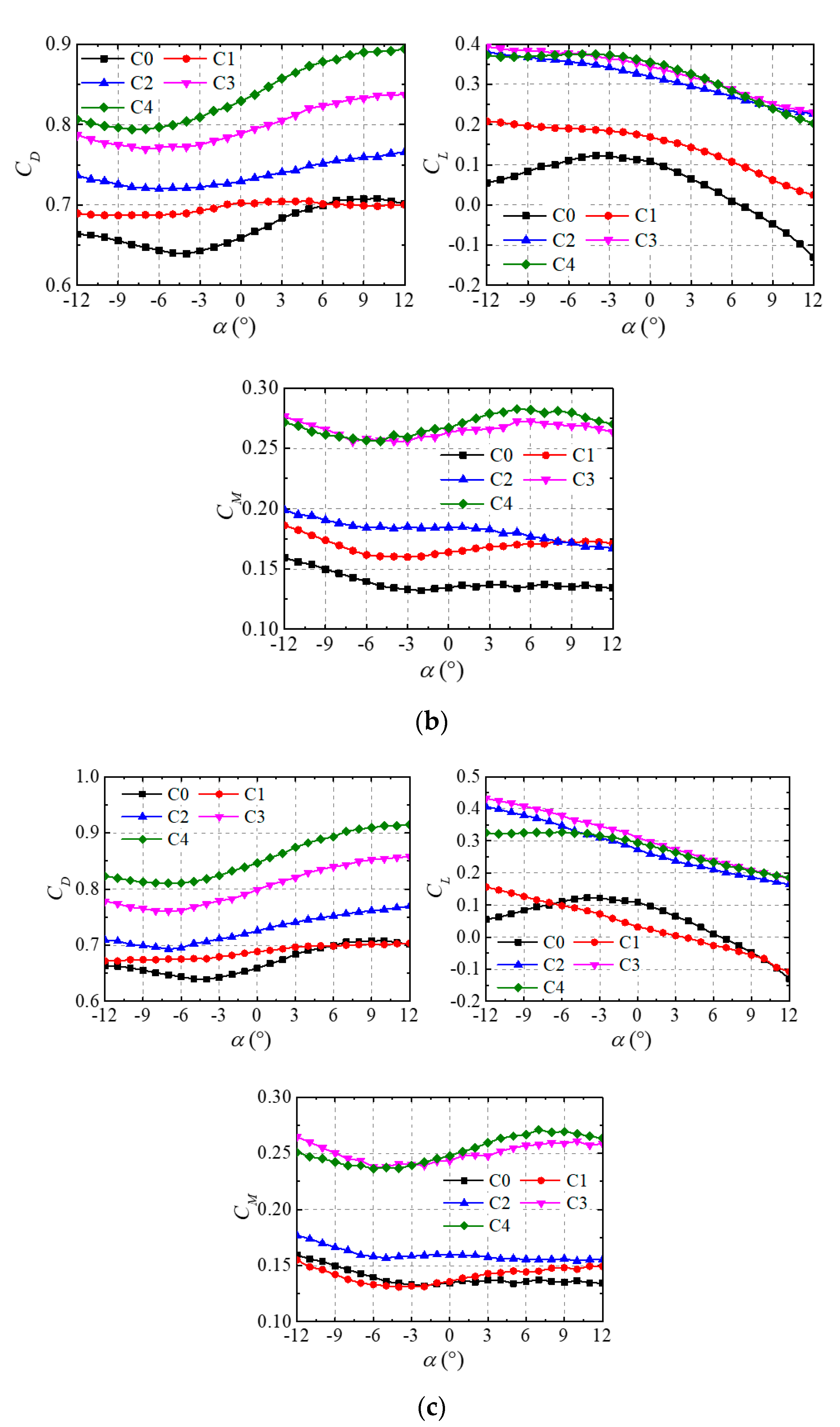
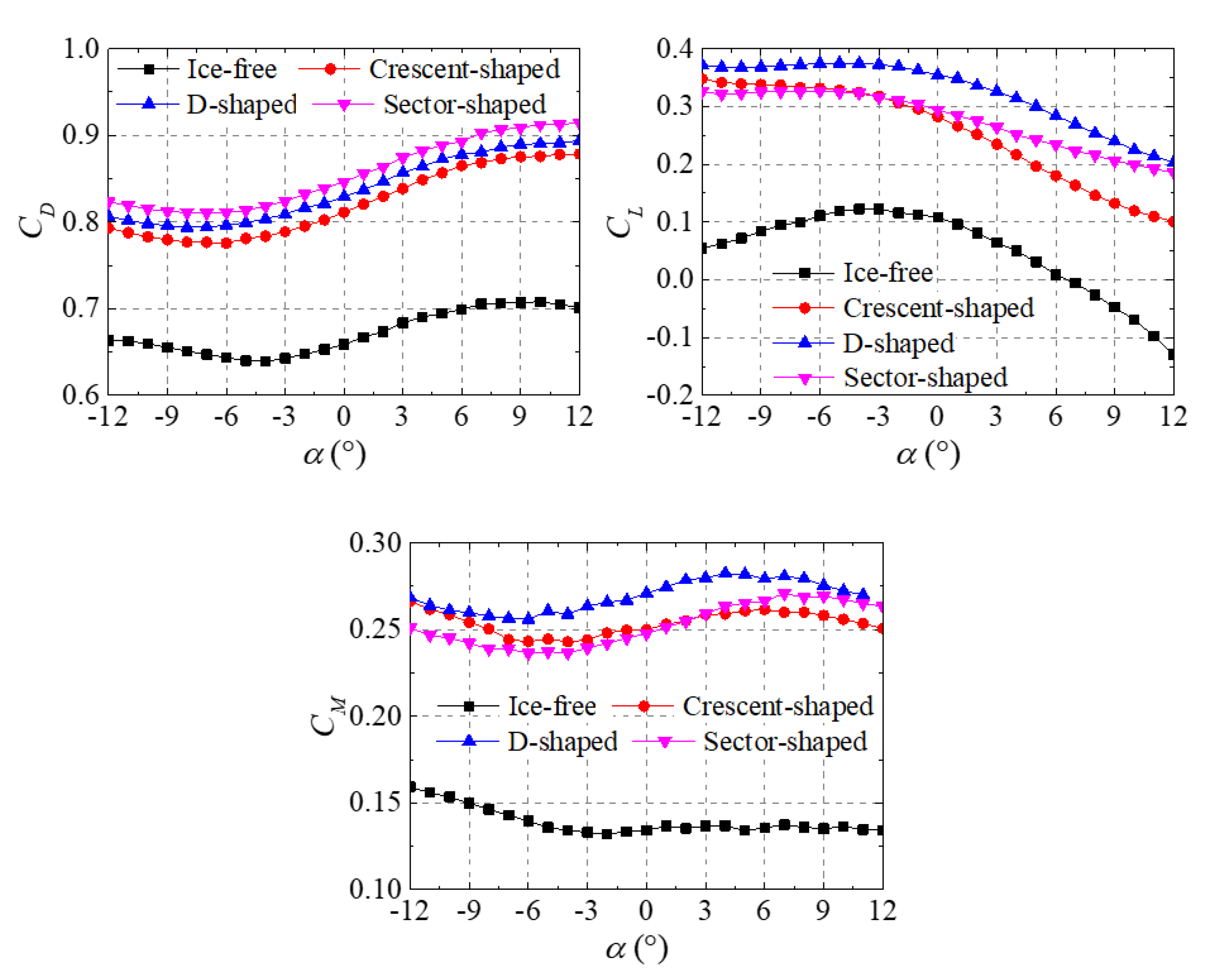
5.2. Aerodynamic Characteristics of Pipeline Girder with Ice Accretion

Aerodynamic force coefficients of section with various ice classes are shown in Figure 25. Because of the asymmetry of the section, the aerodynamics force coefficients were not symmetric between α = −12° to 12°. Aerodynamic force coefficients were significantly affected by ice class. CD increased with increasing ice class, especially for the C3 ice class, which can be ascribed to the increase in the windward area after icing. Aerodynamic force coefficients increased after the pipeline with icicles. CL and CM increased after the guardrail with ice, especially the CM. CL and CM were slightly affected by the ice on guardrail and grate plate. The influence of α on CD for C1 ice class was smaller than that for C2–C4 ice class. CL decreased, and then increased with increasing α for ice-free section, while CL decreased with increasing α for ice-accreted section. For C0 and C1 ice class, CM decreased with increasing α in the range of α = −12° to −3°, and then was almost invariant in the range of α = −4° to 12°. CM decreased with increasing α for C2 ice class. Meanwhile, CM decreased, then increased, and finally decreased with increasing α for C3 and C4 ice class.
Aerodynamic force coefficients of section with various ice types for C4 ice class were shown in Figure 26. Ice accretion had a negligible effect on the variation of the aerodynamic force coefficients with α. CL of the ice-free model gradually increased with increasing α in the range of α = −12° to −2° and then gradually decreased with increasing α in the range of α = −2° to 12°. CL for the pipeline with D-shaped ice was almost invariant in the range of α = −12° to −3° and then gradually decreased with increasing α. The CL values for pipelines with crescent- and sector-shaped ice gradually decreased with increasing α. The CL and CM values for the pipeline with D-shaped ice were larger than those with crescent- and sector-shaped ice. In conclusion, the aerodynamic force coefficients of the iced sections were much higher than those of the ice-free one, which may be ascribed to the large windward area and the asymmetry of the ice-accreted section.

6. Conclusions

For a calm condition with a precipitation rate of 45 mm/h, an air temperature of −7 °C, the dependencies of ice size and shape on the icing duration and some structural properties (including pipeline diameter, inclination angle of wind hanger, inclination angle and size of section steel, and girder geometry) were experimentally investigated in simulated freezing rain environment. Typical ice accretions on pipelines, wind hangers, section steels, and girders of pipeline suspension bridges are summarized. Then the effects of some selected ice accretions on aerodynamic force coefficients of a pipeline bridge girder were further investigated through wind tunnel tests.
With increasing ice thickness, the radial ice profile on the pipeline changed from a thin annular shape to a crescent shape, then to a sector shape, and finally to a D shape. The radial ice thickness and range decreased with increasing pipeline diameter. There were non-uniformities in the lengths and longitudinal center spacing of icicles. The mean icicle length increased with increasing pipeline diameter. The shape of the curved part of the icicle resembled a sickle with thickness of 5 mm, the length of the curved part of the icicle increased with increasing pipeline diameter, and the transverse width increased with increasing icing duration. With increasing icing duration, the shape of linear part of the icicle changed from circular cylinder to circular truncated cone, then to elliptical cone.
The ice shape and thickness on section steels and wind hangers were related to the inclination angle γ. For the wind hanger, icicles are formed when γ = 0°–30°, while iced rivulets are produced when γ > 30°. Icicle length decreased with increasing γ. The areas and thicknesses of the components facing the droplets were increased by the ice on the truss stiffening girder. Size effect of ice accretion on section steels was non-significant. The porosity and thickness of the grate plate decreased and increased with the icing duration, respectively. Ice accretions on the components of the bridge girder had significant interference effects.
The aerodynamic force coefficients of the bridge girder were dependent on the ice type, ice class, and initial angle of attack. The aerostatic analysis of a pipeline suspension bridge might be non-conservative if ice accretion was disregarded, suggesting that the effect of ice accretion should be considered in aerostatic analysis. It is clarified that the ice accretions in this paper should be limited to certain climatic conditions. Further studies are required to investigate the ice accretions on pipeline suspension bridges under more realistic climatic conditions, and to understand their effects on aerodynamic characteristic of the bridges.

Author Contributions

Conceptualization, H.Y. and F.X.; methodology, H.Y.; software, H.Y.; validation, H.Y., M.Z.; formal analysis, H.Y.; investigation, A.Z. and H.Y.; resources, F.X.; data curation, A.Z. and H.Y.; writing—original draft preparation, H.Y.; writing—review and editing, H.Y., M.Z. and F.X.; visualization, F.X.; supervision, F.X.; project administration, F.X.; funding acquisition, F.X. All authors have read and agreed to the published version of the manuscript.

Funding

The research is jointly supported by the National Natural Science Foundation of China (51678115,51978130).

Acknowledgments

The authors would like to thank Lasse Makkonen for his insightful suggestions on this paper.

Conflicts of Interest

The authors declare that they have no known competing financial interests or personal relationships that could have appeared to influence the work reported in this paper.

References

  1. John, A.H.; John, J.G.; Carol, J.C. Pipeline Accident Report; NTS Board: Washington, DC, USA, 2003; NTSB/PAR-03/01 PB2003-916501. [Google Scholar]
  2. Li, J.J.; Zhu, Y.; Chen, G.M. Comparative analysis on emergency management for leakage explosion accidents of urban oil and gas pipeline. J. Saf. Sci. Technol. 2014, 8, 11–15. [Google Scholar]
  3. Gjelstrup, H.; Georgakis, C.; Larsen, A. A preliminary investigation of the hanger vibrations on the Great Belt East Bridge. In Proceedings of the Seventh International Symposium on Cable Dynamics, Vienna, Austria, 1 January 2007. [Google Scholar]
  4. Gjelstrup, H.; Georgakis, C.T.; Larsen, A. An evaluation of iced bridge hanger vibrations through wind tunnel testing and quasi-steady theory. Wind Struct. 2012, 15, 385–407. [Google Scholar] [CrossRef] [Green Version]
  5. Koss, H.H.; Lund, M.S.M. Experimental investigation of aerodynamic instability of iced bridge cable sections. In Proceedings of the 6th European and African Wind Engineering Conference, Cambridge, UK, 7–13 July 2013. [Google Scholar]
  6. Marušić, A.; Kozmar, H. Aerodynamic Behavior of Bridge Cables in Icing Conditions. Ph.D. Thesis, University of Zagreb, Croatia, Balkans, 2014. [Google Scholar]
  7. Demartino, C.; Koss, H.H.; Georgakis, C.T.; Ricciardelli, F. Effects of ice accretion on the aerodynamics of bridge cables. J. Wind Eng. Ind. Aerodyn. 2015, 138, 98–119. [Google Scholar] [CrossRef]
  8. Demartino, C.; Ricciardelli, F. Aerodynamics of nominally circular cylinders: A review of experimental results for Civil Engineering applications. Eng. Struct. 2017, 137, 76–114. [Google Scholar] [CrossRef]
  9. Guo, P.; Li, S.; Wang, D. Effects of aerodynamic interference on the iced straddling hangers of suspension bridges by wind tunnel tests. J. Wind Eng. Ind. Aerodyn. 2019, 184, 162–173. [Google Scholar] [CrossRef]
  10. Jafari, M.; Hou, F.; Abdelkefi, A. Wind-induced vibration of structural cables. Nonlinear Dyn. 2020, 100, 351–421. [Google Scholar] [CrossRef]
  11. Zhang, M.; Xu, F.; Han, Y. Assessment of wind-induced nonlinear post-critical performance of bridge decks. J. Wind Eng. Ind. Aerodyn. 2020, 203, 104251. [Google Scholar] [CrossRef]
  12. Zhang, M.; Xu, F.; Zhang, Z.; Ying, X. Energy budget analysis and engineering modeling of post-flutter limit cycle oscillation of a bridge deck. J. Wind Eng. Ind. Aerodyn. 2019, 188, 410–420. [Google Scholar] [CrossRef]
  13. Kollár, L.E.; Farzaneh, M. Wind-tunnel investigation of icing of an inclined cylinder. Int. J. Heat Mass Transf. 2010, 53, 849–861. [Google Scholar] [CrossRef] [Green Version]
  14. Koss, H.H.; Gjelstrup, H.; Georgakis, C.T. Experimental study of ice accretion on circular cylinders at moderate low temperatures. J. Wind Eng. Ind. Aerodyn. 2012, 104, 540–546. [Google Scholar] [CrossRef]
  15. Demartino, C.; Ricciardelli, F. Aerodynamic stability of ice-accreted bridge cables. J. Fluids Struct. 2015, 52, 81–100. [Google Scholar] [CrossRef]
  16. Lébatto, E.B.; Farzaneh, M.; Lozowski, E.P. Conductor icing: Comparison of a glaze icing model with experiments under severe laboratory conditions with moderate wind speed. Cold Reg. Sci. Technol. 2015, 113, 20–30. [Google Scholar] [CrossRef]
  17. Górski, P.; Pospíšil, S.; Kuznetsov, S.; Tatara, M.; Marušić, A. Strouhal number of bridge cables with ice accretion at low flow turbulence. Wind Struct. 2016, 22, 253–272. [Google Scholar] [CrossRef]
  18. Szilder, K. Theoretical and experimental study of ice accretion due to freezing rain on an inclined cylinder. Cold Reg. Sci. Technol. 2018, 150, 25–34. [Google Scholar] [CrossRef]
  19. Farzaneh, M.; Baker, T.; Bernstorf, A.; Brown, K.; Chisholm, W.A.A.; De Tourreil, C.; Drapeau, J.F.; Fikke, S.; George, J.M.; Gnandt, E.; et al. Insulator icing test methods and procedures: A position paper prepared by the IEEE task force on insulator icing test methods. IEEE Trans. Power Deliv. 2003, 18, 1503–1515. [Google Scholar] [CrossRef]
  20. Farzaneh, M. Insulator flashover under icing conditions. IEEE Trans. Dielectr. Electr. Insul. 2014, 21, 1997–2011. [Google Scholar] [CrossRef]
  21. Lynch, F.T.; Abdollah, K. Effects of ice accretions on aircraft aerodynamics. Prog. Aerosp. Sci. 2002, 37, 669–767. [Google Scholar]
  22. Cao, Y.; Huang, J.; Yin, J. Numerical simulation of three-dimensional ice accretion on an aircraft wing. Int. J. Heat Mass Transf. 2016, 92, 34–54. [Google Scholar] [CrossRef]
  23. Kraj, A.G.; Bibeau, E.L. Phases of icing on wind turbine blades characterized by ice accumulation. Renew. Energy 2010, 35, 966–972. [Google Scholar] [CrossRef]
  24. Han, Y.; Palacios, J.; Schmitz, S. Scaled ice accretion experiments on a rotating wind turbine blade. J. Wind Eng. Ind. Aerodyn. 2012, 109, 55–67. [Google Scholar] [CrossRef]
  25. Chabart, O.; Lilien, J.L. Galloping of electrical lines in wind tunnel facilities. J. Wind Eng. Ind. Aerodyn. 1998, 74, 967–976. [Google Scholar] [CrossRef] [Green Version]
  26. Fukusako, S.; Horibe, A.; Tago, M. Ice accretion characteristics along a circular cylinder immersed in a cold air stream with seawater spray. Exp. Therm. Fluid Sci. 1989, 2, 81–90. [Google Scholar] [CrossRef]
  27. Li, X.M.; Zhu, K.J.; Liu, B. Research of experimental simulation on aerodynamic character for typed iced conductor. Aasri Procedia 2012, 2, 106–111. [Google Scholar]
  28. Kim, J.W.; Sohn, J.H. Galloping simulation of the power transmission line under the fluctuating wind. Int. J. Precis. Eng. Manuf. 2018, 19, 1393–1398. [Google Scholar] [CrossRef]
  29. Górski, P.; Tatara, M.; Pospíšil, S.; Kuznetsov, S. Model investigations of the aerodynamic coefficients of iced cables in cable-stayed bridges. Tech. Trans. 2019, 12, 115–127. [Google Scholar] [CrossRef] [Green Version]
  30. Jones, K.F. Ice Accretion in Freezing Rain (No. CRREL-96-2); Cold Regions Research and Engineering Lab Hanover NH: Hanover, NH, USA, 1996. [Google Scholar]
  31. Langmuir, I.; Blodgett, K.B. A mathematical investigation of water droplet trajectories. In Collected Works of Irving Langmuir; Pergamon Press: Oxford, UK, 1946; Volume 10, pp. 348–393. [Google Scholar]
  32. Finstad, K.J.; Lozowski, E.P.; Makkonen, L. On the median volume diameter approximation for droplet collision efficiency. J. Atmos. Sci. 1988, 45, 4008–4012. [Google Scholar] [CrossRef] [Green Version]
  33. Jeck, R. Representative values of icing-related variables aloft in freezing rain and freezing drizzle. In Proceedings of the 34th Aerospace Sciences Meeting and Exhibit, Reno, NV, USA, 15–18 January 1996; p. 930. [Google Scholar]
  34. Huffman, G.J.; Norman, G.A., Jr. The supercooled warm rain process and the specification of freezing precipitation. Mon. Weather. Rev. 1988, 116, 2172–2182. [Google Scholar] [CrossRef]
  35. Jiang, X.L.; Yi, H. Ice Accretion and Protection of Transmission Lines; China Electric Power Press: Beijing, China, 2002. [Google Scholar]
  36. Makkonen, L. Modeling power line icing in freezing precipitation. Atmos. Res. 1998, 46, 131–142. [Google Scholar] [CrossRef]
  37. Makkonen, L.; Fujii, Y. Spacing of icicles. Cold Reg. Sci. Technol. 1993, 21, 317–322. [Google Scholar] [CrossRef]
  38. International Organization for Standardization. ISO 12494: Atmospheric Icing of Structures, 2nd ed.; ISO: Geneva, Switzerland, 2017. [Google Scholar]
  39. Maeno, N.; Makkonen, L.; Nishimura, K.; Kosugi, K.; Takahashi, T. Growth rates of icicles. J. Glaciol. 1994, 40, 319–326. [Google Scholar] [CrossRef] [Green Version]
  40. Niu, L.; Huang, F.; Wang, G.F. Creation of a New Freezing Rain Genesis Potential Index over China. Period. Ocean Univ. China 2015, 45, 8–15. [Google Scholar]
  41. Makkonen, L. Models for the growth of rime, glaze, icicles and wet snow on structures. Philos. Trans. R. Soc. Ser. A Math. Phys. Eng. Sci. 2000, 358, 2913–2939. [Google Scholar] [CrossRef]
  42. Taylor, G. The instability of liquid surfaces when accelerated in a direction perpendicular to their planes. Proc. R. Soc. Lond. 1950, 201, 192–196. [Google Scholar]
  43. De Bruyn, J.R. On the formation of periodic arrays of icicles. Cold Reg. Sci. Technol. 1997, 25, 225–229. [Google Scholar] [CrossRef]
  44. Makkonen, L. A model of icicle growth. J. Glaciol. 1988, 34, 64–70. [Google Scholar] [CrossRef] [Green Version]
  45. Maeno, N.; Takahashi, T. Studies on icicles. I. General aspects of the structure and growth of an icicle. Low Temp. Sci. 1984, 43, 125–138. [Google Scholar]
  46. Makkonen, L. Heat transfer and icing of a rough cylinder. Cold Reg. Sci. Technol. 1985, 10, 105–116. [Google Scholar] [CrossRef]
Figure 1. Schematic diagram of ice shapes: (a) trilateral shape, (b) crescent shape, (c) ellipse shape, (d) D shape, (e) D shape, (f) sector shape, (g) crescent shape.
Applsci 10 07167 g001
Figure 2. Experiment setup.
Applsci 10 07167 g002
Figure 3. Schematic diagram of cross section (unit: mm): (a) girder A, (b) girder B and (c) girder C.
Applsci 10 07167 g003
Figure 4. Symbol definition of ice accretion on pipeline.
Applsci 10 07167 g004
Figure 5. Profiles and side views of ice accretion on pipelines (N = 160): (a) D = 25 mm, (b) D = 50 mm, (c) D = 100 mm, (d) D = 150 mm, (e) D = 200 mm, (f) D = 300 mm, (g) D = 400 mm, (h) D = 600 mm, (i) D = 800 mm, and (j) D = 1000 mm.
Applsci 10 07167 g005
Figure 6. Radial ice size: (a) icing range and (b) ice thickness at θ = 0°.
Applsci 10 07167 g006
Figure 7. Icicle size of pipeline: (a) mean length and (b) center-to-center spacing.
Applsci 10 07167 g007
Figure 8. Profiles of ice accretions for various N (D = 25 mm).
Applsci 10 07167 g008
Figure 9. Profiles of ice accretions for various N (D = 50 mm).
Applsci 10 07167 g009
Figure 10. Profiles of ice accretions for various N (D = 150 mm).
Applsci 10 07167 g010
Figure 11. Profiles of ice accretions for various N (D = 1000 mm).
Applsci 10 07167 g011aApplsci 10 07167 g011b
Figure 12. Thickness of radial ice at various N: (a) D = 25 mm, (b) D = 50 mm, (c) D = 100 mm, (d) D = 150 mm, (e) D = 200 mm, (f) D = 300 mm, (g) D = 400 mm, (h) D = 600 mm, (i) D = 800 mm, and (j) D = 1000 mm.
Applsci 10 07167 g012aApplsci 10 07167 g012b
Figure 13. μ and l at different N: (a) D = 150 mm, and (b) D = 1000 mm.
Applsci 10 07167 g013
Figure 14. Engineering geometric models of radial ice: (a) annular shaped, (b) crescent shaped, (c) sector shaped, and (d) D shaped.
Applsci 10 07167 g014
Figure 15. Some details of the icicle: (a) D = 200 mm, and (b) D = 1000 mm.
Applsci 10 07167 g015
Figure 16. Profile and lateral views of ice accreted cylinder for various γ (N = 100): (a) D = 50 mm, (b) D = 25 mm.
Applsci 10 07167 g016aApplsci 10 07167 g016b
Figure 17. Ice sizes of wind hangers versus γ (N = 100): (a) maximum δ0, and (b) l.
Applsci 10 07167 g017
Figure 18. Profiles or side views of ice accretions for section steel (N = 80): (a) L100 for γ = 0°, (b) L100 for γ = 90°, (c) U140 for γ = 0°, (d) U140 for γ = 90°, and (e) Ⅰ200 for γ = 0°.
Applsci 10 07167 g018
Figure 19. Side views of ice accretions for L100 and γ = 90°.
Applsci 10 07167 g019
Figure 20. Side views of icing sectional model: (a) girder A, (b) girder B, and (c) girder C.
Applsci 10 07167 g020aApplsci 10 07167 g020b
Figure 21. Ice accretion of grate plate: (a) girder A and (b) girder B.
Applsci 10 07167 g021
Figure 22. Schematic diagram of iced pipeline and guardrail (mm): (a) pipeline with crescent-shaped ice, (b) pipeline with D-shaped ice, (c) pipeline with sector-shaped ice, and (d) guardrail with crescent-shaped ice.
Applsci 10 07167 g022
Figure 23. Side views and sizes of icicles (mm): (a) pipeline with crescent-shaped ice, (b) pipeline with D- and sector-shaped ice, and (c) guardrail with crescent-shaped ice.
Applsci 10 07167 g023aApplsci 10 07167 g023b
Figure 24. Pipeline girder sectional models: (a) ice-free, (b) crescent-shaped ice for C4, (c) D-shaped ice for C1, and (d) sector-shaped ice for C4.
Applsci 10 07167 g024
Figure 25. Aerodynamic force coefficients of section with various ice classes (U = 15.5 m/s): (a) pipeline with crescent-shaped ice, (b) pipeline with D-shaped ice, (c) pipeline with sector-shaped ice.
Applsci 10 07167 g025aApplsci 10 07167 g025b
Figure 26. Aerodynamic force coefficients of section with various ice types for C4 ice class (U = 15.5 m/s).
Applsci 10 07167 g026
Table 1. Summary of icing test cases.
Section TypeSection Size (mm)Length L (mm)Angle γ (°)Spraying Times N
Circular cylinderØ1000, Ø800, Ø60010000240
Circular cylinderØ400, Ø300, Ø200, Ø150, Ø100, Ø50, Ø2510000160
Circular cylinderØ150, Ø100, Ø50, Ø25100010, 20, 30,40, 50, 6080
Angle steelL160, L100, L5010000, 18080
U-steelU200, U140, U10010000, 9080
I-beamI250, I200, I1001000080
Girder A324 × 417 (scale 1: 6)1030030
Girder B536 × 336 (scale 1: 5)1000030
Girder C625 × 453 (scale 1:6. 4)1200030
Table 2. Ice mean size of section steel for N = 80 (unit: mm).
CasesL160L100L50U200U140U100Ⅰ250Ⅰ200Ⅰ100
90°90°90°90°90°90°
Bt-16-19-19191921211820252819
Bb27-29-29-9-9-9-241912
Bs1441351539-11-10----
lt-244-200-171 - - -
lb170-221-148-174-135-134-118115172
ls45169420868175200188178197174170---
st-20-38-19172122241823181822
sb25-18-25-20-25-21-211926
ss11241320192022-23-18----
Publisher’s Note: MDPI stays neutral with regard to jurisdictional claims in published maps and institutional affiliations.

