Applying the Cracking Elements Method for Analyzing the Damaging Processes of Structures with Fissures

Abstract

In this work, the recently proposed cracking elements method (CEM) is used to simulate the damage processes of structures with initial imperfections. The CEM is built within the framework of the conventional finite element method (FEM) and is formally similar to a special type of finite element. Disconnected piecewise cracks are used to represent the crack paths. With the advantage of the CEM for which both the initiation and propagation of cracks can be captured naturally, we numerically study uniaxial compression tests on specimens with multiple joints and fissures, where the cracks may propagate from the tips or from other unexpected positions. Although uniaxial compression tests are considered, tensile damage criteria are mainly used in the numerical model. On the one hand, the results demonstrate the robustness and effectiveness of the CEM, while, on the other hand, some drawbacks of the present model are demonstrated, indicating directions for future work.

1. Introduction

Great engineering practices include the prediction and prevention of the propagation and initiation of cracks in structures with complex initial imperfections, such as rock masses with joints and concrete structures with early age cracks. When these structures are subjected to complex loading conditions, the existing cracks may propagate further, and new cracks may emerge. For these structures, analytical and empirical analyses are not sufficient to ensure their safety and durability. Numerical tools are highly preferable.

With the understanding of continuum-discontinuous theory and developments in computing power, many sophisticated numerical methods have been proposed in recent decades. These methods can be built in a continuum or discrete framework [1,2,3] and can introduce damage degrees [4,5] or crack openings (crack widths) [6,7] as the new degrees of freedom. They can localize the damage [8,9], consider nonlocal effects [10,11], or even assume long-range forces [12,13]. A crack can be explicitly represented by moving boundaries [14,15,16,17] or implicitly embedded to avoid remeshing [18,19,20,21]. The cracked domain can be discretized with elements [6,22,23] or particles [24,25,26]. In summary, these methods have advantages as well as disadvantages for different problems. Hence, a problem-oriented selection procedure would be helpful.

Returning to our problem, to analyze the damaging processes of structures with initial imperfections, we need a method that is capable of capturing the initiation as well as the propagation of cracks. Since we do not focus on the stress state, such as the stress intensity factor around specific crack tips, numerical methods using remeshing [15,27,28], and nodal enrichment methods, such as the extended finite element method (XFEM) [18,29,30,31] and the numerical manifold method (NMM) [32,33,34,35], are not considered for simplicity. Furthermore, crack openings are very important for analyzing the durability of structures, and quasi-static loading conditions are considered. Hence, we do not use damage degree-based methods such as the phase field method [36,37,38,39], mixed mode model [40,41,42,43], equivalent lattice models [44,45,46,47], and peridynamic-based methods [48,49,50,51]. Finally, we hope that multiple cracks can be efficiently tracked simultaneously and that complicated crack tracking strategies [52,53] can be avoided. The cracking elements method (CEM) [54,55,56,57] is the chosen numerical tool.

The CEM is a novel numerical approach belonging to the family of strong discontinuity embedded approaches (SDAs) [58,59,60,61]. CEM uses Statically Optimal Symmetric (SOS) formulation [62]. Unlike the other SDAs, it introduces disconnected piecewise cracking segments appearing in the center point of each cracked element to represent crack paths, similar to the cracking particle method (CPM) [63,64,65,66]. Hence, it does not need to distinguish crack tip elements and crack passing elements, which naturally captures the initiation and propagation of cracks. The crack orientation is determined locally, greatly reducing the computing effort. Moreover, [56] shows that a cracking element can be treated as a special type of finite element, which is formally like a 9-node quadrilateral element (or 7-node triangular element). Hence, this idea can be implemented easily in the conventional FEM framework.

In this work, the CEM is used for simulating the damaging processes of brittle structures with joints and fissures. The numerically obtained results are compared with the experimental results, where the cracks do not always propagate from the tips of joints. In particular, uniaxial compression tests are considered, while we only use tensile damage criteria in our numerical model. On the one hand, satisfactory results are obtained in most cases where the cracking patterns observed in the experiments are numerically-reproduced. On the other hand, the differences between the numerical and experimental results will guide us in conducting our future research.

The remaining parts of this paper are organized as follows: In Section 2, the constitutive relationship and the formulation of the CEM are presented. The elemental stiffness matrix and residual vector are provided, showing that the CEM is very similar to the conventional FEM. The numerical studies are provided in Section 3 and are compared to the experimental results. This paper closes with concluding remarks in Section 4.

2. Methods

Since the details of the CEM were proposed in [56,57] in matrix form, only a brief introduction will be provided in this section. By providing the elemental stiffness matrix and residual vector of uncracked and cracked elements, we will demonstrate the ease of implementing the CEM in the FEM framework.

2.1. Traction–Separation Law

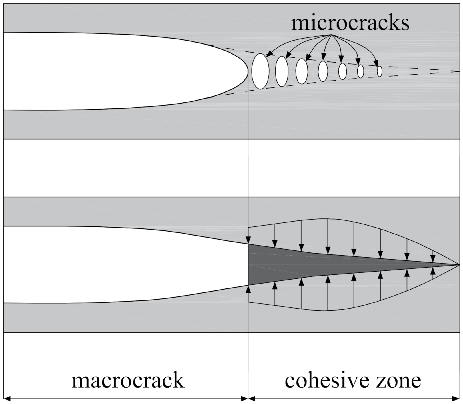
In this work, cohesive crack is considered, which is consistent with the cohesive zone model. After the crack initiates, the traction across the two crack surfaces will drop from a prescribed value such as tensile strength to zero with the opening of crack [67], see Figure 1. The relationship between the traction and the crack opening is described by the so called traction–separation law.

In this work, the exponential mixed-mode traction–separation law [68,69,70] is used in the CEM. Under 2D conditions, the equivalent crack opening is defined as

$${\zeta }_{eq}=\sqrt{{\zeta }_n^2+{\zeta }_t^2},$$

(1)

where ${\zeta }_n$ and ${\zeta }_t$ are the crack openings (as unknowns) along the normal and parallel directions, respectively, of the crack path and the corresponding unit vectors are denoted as $\mathbf{n}={\left[n_x,n_y\right]}^T$ and $\mathbf{t}={\left[t_x,t_y\right]}^T$. Clearly, $n_x{t}_x+n_y{t}_y=0$. The traction components along $\mathbf{n}$ and $\mathbf{t}$, namely, $T_n$ and $T_t$, respectively, are obtained as

$$\begin{array}{cc}\hfill & T_n=T_{eq}\frac{{\zeta }_n}{{\zeta }_{eq}},T_t=T_{eq}\frac{{\zeta }_t}{{\zeta }_{eq}}\hfill \\ \hfill & with\hfill \\ \hfill & T_{eq}\left({\zeta }_{eq}\right)=\left\{\begin{array}{cc}TL\left({\zeta }_{eq}\right)=f_{t}exp\left(-\frac{f_t}{G_f}{\zeta }_{eq}\right),\hfill & \mathrm{l}\mathrm{o}\mathrm{a}\mathrm{d}\mathrm{i}\mathrm{n}\mathrm{g},\hfill \\ TU\left({\zeta }_{eq}\right)=\frac{T_{mx}}{{\zeta }_{mx}}{\zeta }_{eq},\hfill & \mathrm{u}\mathrm{n}\mathrm{l}\mathrm{o}\mathrm{a}\mathrm{d}\mathrm{i}\mathrm{n}\mathrm{g}/\mathrm{r}\mathrm{e}\mathrm{l}\mathrm{o}\mathrm{a}\mathrm{d}\mathrm{i}\mathrm{n}\mathrm{g},\hfill \end{array}\right.\hfill \end{array}$$

(2)

where $f_t$ is the uniaxial tensile strength, $G_f$ is the fracture energy, ${\zeta }_{mx}$ is the size of the maximum opening that the crack has ever experienced, and $T_{mx}=TL\left({\zeta }_{mx}\right)$ is the corresponding traction. The traction–separation law indicates that the CEM is consistent with the conventional cohesive zone model as a crack opening-based model but not a damage degree-based model.

Correspondingly, the relationship between the traction differentials $d{T}_n$ and $d{T}_t$ and the crack openings ${\zeta }_n$ and ${\zeta }_t$ are described by

$$\mathbf{D}\left[\begin{array}{c}d{\zeta }_n\\ d{\zeta }_t\end{array}\right]=\left[\begin{array}{c}d{T}_n\\ d{T}_t\end{array}\right],$$

(3)

with

$$\begin{array}{c}\mathbf{D}=-\frac{T_{eq}}{{\zeta }_{eq}}\left[\begin{array}{cc}\frac{{\zeta }_n^2}{{\zeta }_{eq}^2}+\frac{f_t{\zeta }_n^2}{G_f{\zeta }_{eq}}-1& \frac{{\zeta }_n{\zeta }_t}{{\zeta }_{eq}^2}+\frac{f_t{\zeta }_n{\zeta }_t}{G_f{\zeta }_{eq}}\\ \frac{{\zeta }_n{\zeta }_t}{{\zeta }_{eq}^2}+\frac{f_t{\zeta }_n{\zeta }_t}{G_f{\zeta }_{eq}}& \frac{{\zeta }_t^2}{{\zeta }_{eq}^2}+\frac{f_t{\zeta }_t^2}{G_f{\zeta }_{eq}}-1\end{array}\right]\mathrm{f}\mathrm{o}\mathrm{r} \mathrm{l}\mathrm{o}\mathrm{a}\mathrm{d}\mathrm{i}\mathrm{n}\mathrm{g},\hfill \\ and\hfill \\ \mathbf{D}=\frac{T_{mx}}{{\zeta }_{mx}}\left[\begin{array}{cc}1& 0\\ 0& 1\end{array}\right]\mathrm{f}\mathrm{o}\mathrm{r} \mathrm{u}\mathrm{n}\mathrm{l}\mathrm{o}\mathrm{a}\mathrm{d}\mathrm{i}\mathrm{n}\mathrm{g}/\mathrm{r}\mathrm{e}\mathrm{l}\mathrm{o}\mathrm{a}\mathrm{d}\mathrm{i}\mathrm{n}\mathrm{g},\hfill \end{array}$$

(4)

in which $\mathbf{D}$ obviously remains symmetric.

On the other hand, some other types of traction–separation laws, such as linear, bilinear, and hyperbolic laws, can also be applied, but this has not yet been attempted. We prefer the exponential law because (i) it only needs two parameters, $f_t$ and $G_f$, both of which have strong physical meanings and can be obtained experimentally by standard tests; and (ii) it has $C^{\infty }$ continuity, making $\mathbf{D}$ very simple.

2.2. Elemental Formulation

In our early work, such as [54,55], we focused on the deduction processes of the CEM framework by introducing strain localization [71,72] and enhanced assumed strains (EASs) [73,74,75] in which many complicated tensors are assumed. On the one hand, this paved the way for the current method; on the other hand, it reduced the readability. In this work, only the 2D condition is considered. We use Voigt notation to represent all second- and fourth-order tensors with their corresponding vector and matrix forms [76]. Moreover, from a practical point of view, we will directly provide the elemental formulation of uncracked and cracking elements for comparison.

First, for the nonlinear analysis, the standard Newton–Raphson (N–R) iteration procedure is used. The global vector of the degrees of freedom is represented with the symbol $\mathsf{U}=\bigcup {\mathbf{U}}^{\left(e\right)}$, where $\bigcup \left(·\right)$ denotes the assemblage of the elemental matrix or vector in the global form. For load step i in iteration step j, the following equation is introduced:

$$\begin{array}{cccc}{\mathsf{U}}_{i,j}=& \underbrace{{\mathsf{U}}_{i-1}+\Delta {\mathsf{U}}_{j-1}}& +& \underbrace{\Delta \Delta \mathsf{U}}\\ & \mathrm{k}\mathrm{n}\mathrm{o}\mathrm{w}\mathrm{n}& & \mathrm{u}\mathrm{n}\mathrm{k}\mathrm{n}\mathrm{o}\mathrm{w}\mathrm{n}\end{array}.$$

(5)

Then, the linearized balance equation is represented as

$${\mathsf{K}}_{j-1}\Delta \Delta \mathsf{U}={\mathsf{R}}_{j-1},$$

(6)

where ${\mathsf{K}}_{j-1}$ is the global stiffness matrix, with $\mathsf{K}=\bigcup {\mathbf{K}}^{\left(e\right)}$. ${\mathsf{R}}_{j-1}$ the residual vector, with $\mathsf{R}=\bigcup {\mathbf{R}}^{\left(e\right)}$. ${\mathsf{R}}_{j-1}$ being a function of $\left({\mathsf{U}}_{i-1}+\Delta {\mathsf{U}}_{j-1}\right)$. Then, for the elemental stiffness matrix ${\mathbf{K}}^{\left(e\right)}$ and the residual vector ${\mathbf{R}}^{\left(e\right)}$ of the uncracked element and cracking element, we have

2.2.1. Uncracked Element

For an uncracked element e, its unknown vector is ${\mathbf{U}}^{\left(e\right)}={\left[{\mathbf{u}}_1\cdots {\mathbf{u}}_n\right]}^T$, in which n is the node number. Its shape function is denoted as ${\mathbf{N}}^{\left(e\right)}$, with $\mathbf{u}\left(\mathbf{x}\right)={\mathbf{N}}^{\left(e\right)}\left(\mathbf{x}\right){\mathbf{U}}^{\left(e\right)}$, and its B matrix is denoted as ${\mathbf{B}}^{\left(e\right)}=\nabla {\mathbf{N}}^{\left(e\right)}$. Neglecting the nonlinear effects of the material, its elemental stiffness matrix ${\mathbf{K}}^{\left(e\right)}$ is obtained as

$${\mathbf{K}}_{j-1}^{\left(e\right)}={\mathbf{K}}^{\left(e\right)}=\int {\left({\mathbf{B}}^{\left(e\right)}\right)}^T{\mathbf{C}}^{\left(e\right)}{\mathbf{B}}^{\left(e\right)}d\left(e\right),$$

(7)

where ${\mathbf{C}}^{\left(e\right)}$ is the matrix form of the elastic tensor. Its residual vector at iteration step $j-1$, ${\mathbf{R}}_{j-1}^{\left(e\right)}$, is obtained as

$${\mathbf{R}}_{j-1}^{\left(e\right)}={\mathbf{F}}^{\left(e\right)}-{\mathbf{K}}^{\left(e\right)}\left({\mathbf{U}}_{i-1}+\Delta {\mathbf{U}}_{j-1}\right),$$

(8)

where ${\mathbf{F}}^{\left(e\right)}$ represents the loading forces on the corresponding nodes. Because ${\mathbf{K}}^{\left(e\right)}$ will not change during the iteration, only one iteration step is needed for convergence.

2.2.2. Cracking Element

On the other hand, for the cracking element, its unknown vector is defined as ${\mathbf{U}}^{\left(e\right)}={\left[{\mathbf{u}}_1\cdots {\mathbf{u}}_n,{\zeta }_n,{\zeta }_t\right]}^T$. Its B matrix is extended to

$${\mathbf{B}}^{\left(e\right)}=\left[\nabla {\mathbf{N}}^{\left(e\right)},{\mathbf{B}}_{\zeta }\right],$$

(9)

where ${\mathbf{N}}^{\left(e\right)}$ is the original shape function, and

$${\mathbf{B}}_{\zeta }^{\left(e\right)}=-{\left(l_c^{\left(e\right)}\right)}^{-1}\left[\begin{array}{cc}{n}_x^{\left(e\right)}·n_x^{\left(e\right)}& n_x^{\left(e\right)}·t_x^{\left(e\right)}\\ n_y^{\left(e\right)}·n_y^{\left(e\right)}& n_y^{\left(e\right)}·t_y^{\left(e\right)}\\ 2n_x^{\left(e\right)}·n_y^{\left(e\right)}& n_x·t_y^{\left(e\right)}+n_y^{\left(e\right)}·t_x^{\left(e\right)}\end{array}\right],$$

(10)

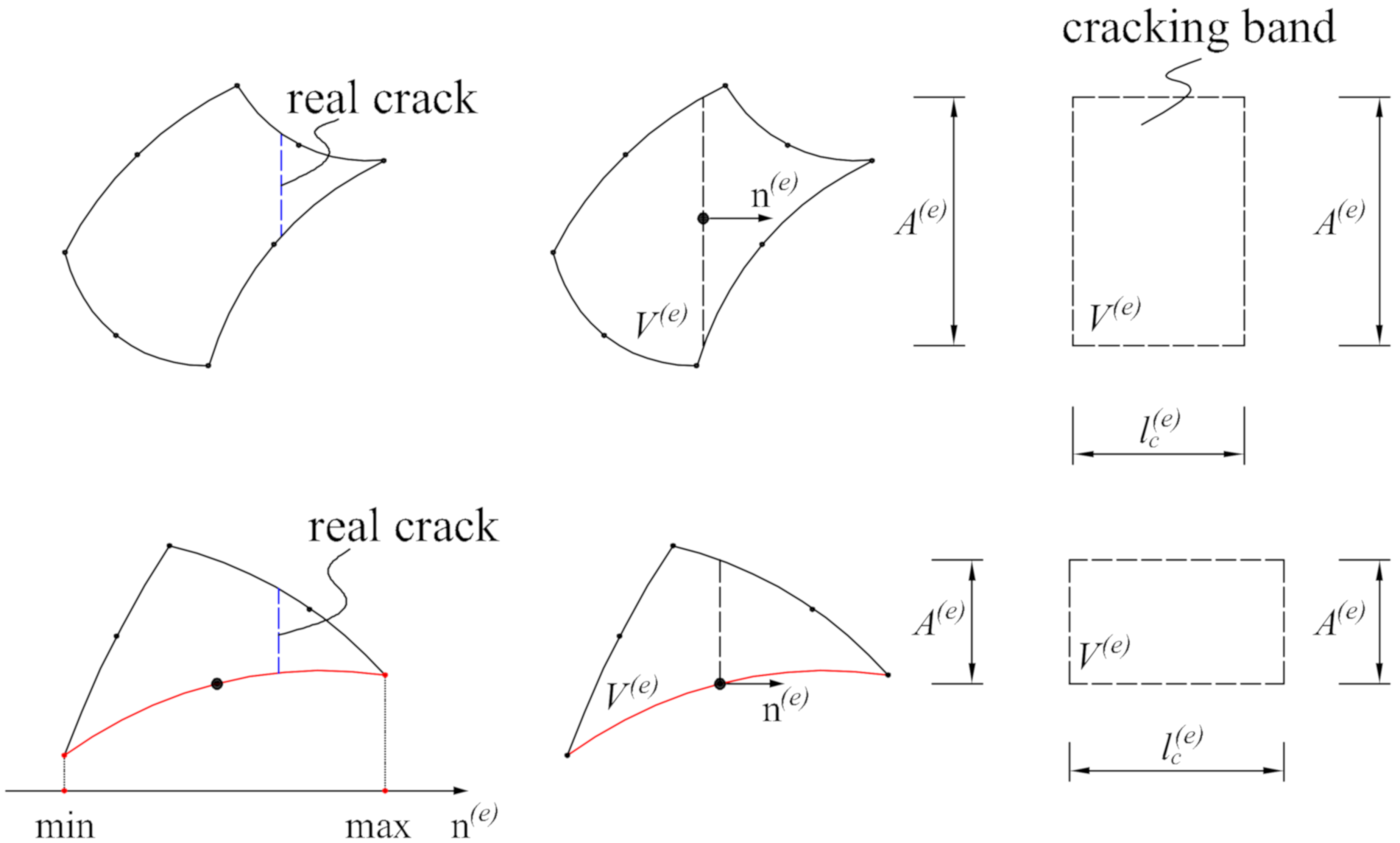
where the element-dependent parameter $l_c^{\left(e\right)}$ is obtained as $l_c^{\left(e\right)}=V^{\left(e\right)}/A^{\left(e\right)}$, $V^{\left(e\right)}$ denotes the volume of element e and $A^{\left(e\right)}$ stands for the surface area of an equivalent crack parallel to the real crack. In fact, $l_c$ corresponds to the classic characteristic length [77,78]. Here, the determination of $A^{\left(e\right)}$ for the 8-node quadrilateral (Q8) and 6-node triangular (T6) elements is slightly different insofar as the equivalent crack passes through the center point of Q8 but through the midpoint of one edge of T6; see Figure 2. More details can be found in [56,57].

Its elemental stiffness matrix ${\mathbf{K}}^{\left(e\right)}$ can be obtained as

$${\mathbf{K}}_{j-1}^{\left(e\right)}=\int {\left({\mathbf{B}}^{\left(e\right)}\right)}^T{\mathbf{C}}^{\left(e\right)}{\mathbf{B}}^{\left(e\right)}d\left(e\right)+\left[\begin{array}{cc}\mathbf{0}& \mathbf{0}\\ \mathbf{0}& A^{\left(e\right)}{\mathbf{D}}^{\left(e\right)}\end{array}\right].$$

(11)

The crack orientation ($\mathbf{n}$) and crack openings will change during the iteration. ${\mathbf{K}}_{j-1}^{\left(e\right)}$ of the cracking element is not constant. Its residual vector at iteration step $j-1$, ${\mathbf{R}}_{j-1}^{\left(e\right)}$ is obtained as

$${\mathbf{R}}_{j-1}^{\left(e\right)}=\left[\begin{array}{c}{\mathbf{F}}^{\left(e\right)}\\ -A^{\left(e\right)}{\mathbf{T}}^{\left(e\right)}\end{array}\right]-{\mathbf{S}}_{j-1}^{\left(e\right)}\left({\mathbf{U}}_{i-1}+\Delta {\mathbf{U}}_{j-1}\right),$$

(12)

where ${\mathbf{T}}^{\left(e\right)}={\left[T_n^{\left(e\right)},T_t^{\left(e\right)}\right]}^T$ (see Equation (2)) and ${\mathbf{S}}_{j-1}$ is a designed unsymmetrical matrix

$${\mathbf{S}}_{j-1}=\left[\begin{array}{cc}\int {\left(\nabla {\mathbf{N}}^{\left(e\right)}\right)}^T{\mathbf{C}}^{\left(e\right)}\left(\widehat{\nabla {\mathbf{N}}^{\left(e\right)}}\right)d\left(e\right)& \int {\left(\nabla {\mathbf{N}}^{\left(e\right)}\right)}^T{\mathbf{C}}^{\left(e\right)}{\mathbf{B}}_{\zeta }^{\left(e\right)}d\left(e\right)\\ V^{\left(e\right)}{\left({\mathbf{B}}_{\zeta }^{\left(e\right)}\right)}^T{\mathbf{C}}^{\left(e\right)}\left(\widehat{\nabla {\mathbf{N}}^{\left(e\right)}}\right)& V^{\left(e\right)}{\left({\mathbf{B}}_{\zeta }^{\left(e\right)}\right)}^T{\mathbf{C}}^{\left(e\right)}{\mathbf{B}}_{\zeta }^{\left(e\right)}\end{array}\right],$$

(13)

where $\widehat{\nabla {\mathbf{N}}^{\left(e\right)}}$ is the value of $\nabla {\mathbf{N}}^{\left(e\right)}$ at the center point of element e.

In summary, the elemental formulations of an uncracked element and cracking element are very similar. Once an uncracked element becomes a cracking element, its cracks can be captured by replacing its elemental stiffness matrix and residual vector, provided in Equations (7) and (8), with the new form provided in Equations (11) and (12). Formally, a quadrilateral cracking element is similar to a 9-node quadrilateral element (transformed from Q8), and a triangular cracking element is similar to a 7-node triangular element (transformed from T6). The displacement degrees of freedom of the center point are now used to represent the normal and shear crack openings.

2.3. Determination of $\mathbf{n}$, Crack Propagation, and Initiation

A local criterion was first proposed in [54] for determining $\mathbf{n}$, in which $\mathbf{n}$ is assumed to be the first eigenvector of the total strain $\widehat{{\epsilon }^{\left(e\right)}}$, which is determined by

$$\widehat{{\epsilon }^{\left(e\right)}}=\left[\begin{array}{c}{\widehat{\epsilon }}_x^{\left(e\right)}\\ {\widehat{\epsilon }}_y^{\left(e\right)}\\ {\widehat{\gamma }}_{xy}^{\left(e\right)}\end{array}\right]=\widehat{\nabla {\mathbf{N}}^{\left(e\right)}}\left[\begin{array}{c}{\mathbf{u}}_1\\ ⋮\\ {\mathbf{u}}_n\end{array}\right],$$

(14)

which is independent of ${\zeta }_n$ and ${\zeta }_t$. After solving for the eigenvalue and eigenvector, we obtain

$$\begin{array}{cc}\hfill & \left[\begin{array}{c}{n}_x^{\left(e\right)}\\ n_y^{\left(e\right)}\end{array}\right]=\left[\begin{array}{c}a/\sqrt{a^2+b^2}\\ b/\sqrt{a^2+b^2}\end{array}\right]\hfill \\ \hfill & \mathrm{where}\hfill \\ \hfill & a=\frac{{\widehat{\gamma }}_{xy}^{\left(e\right)}}{2}\hfill \\ \hfill & b=\frac{{\widehat{\epsilon }}_y^{\left(e\right)}-{\widehat{\epsilon }}_x^{\left(e\right)}+\sqrt{{\left({\widehat{\epsilon }}_x^{\left(e\right)}-{\widehat{\epsilon }}_y^{\left(e\right)}\right)}^2+{\left({\widehat{\gamma }}_{xy}^{\left(e\right)}\right)}^2}}{2}.\hfill \end{array}$$

(15)

In the framework of the CEM, the elements will experience cracking one after another. Crack propagation is always checked first; then, crack initiation is considered. This procedure is based on the idea that, when the extensions of the existing cracks cannot fully release the extra stress, new cracks will appear. This procedure was used to capture the dynamic crack propagation in [55] where the branching and intersection of cracks are successfully captured.

First, an index ${\varphi }_{RK}^{\left(e\right)}$ is introduced as

$${\varphi }_{RK}^{\left(e\right)}={\left[\begin{array}{c}{n}_x^{\left(e\right)}·n_x^{\left(e\right)}\\ n_y^{\left(e\right)}·n_y^{\left(e\right)}\\ 2n_x^{\left(e\right)}·n_y^{\left(e\right)}\end{array}\right]}^T{\mathbf{C}}^{\left(e\right)}\left[\begin{array}{c}{\widehat{\epsilon }}_x^{\left(e\right)}\\ {\widehat{\epsilon }}_y^{\left(e\right)}\\ {\widehat{\gamma }}_{xy}^{\left(e\right)}\end{array}\right]-f_t^{\left(e\right)}$$

(16)

Then, the computing procedure below is conducted.

1.

The uncracked domain is divided into two subdomains, (i) a propagation domain and (ii) a crack root domain, based on a simple rule: when an element shares at least one edge with a cracking element, it belongs to the propagation domain; otherwise, it is in the crack root domain. Clearly, in the beginning, the whole domain is the crack root domain.

2.

Find $\left\{max\left\{{\varphi }_{RK}^{\left(e\right)}\right\}\right\}$ in the propagation domain. If $\left\{max\left\{{\varphi }_{RK}^{\left(e\right)}\right\}\right\}>0$, the element becomes a cracking element; then, the two subdomains will be updated, the N–R iteration will be run, and this step will be conducted again. If $\left\{max\left\{{\varphi }_{RK}^{\left(e\right)}\right\}\right\}\le 0$, go to the next step.

3.

Find $\left\{max\left\{{\varphi }_{RK}^{\left(e\right)}\right\}\right\}$ in the crack root domain. If $\left\{max\left\{{\varphi }_{RK}^{\left(e\right)}\right\}\right\}>0$, the element becomes a cracking element; then, the two subdomains will be updated, the N–R iteration will be run and step 2 will be conducted again. If $\left\{max\left\{{\varphi }_{RK}^{\left(e\right)}\right\}\right\}\le 0$, this loading step is considered to converge.

A detailed flowchart can be found in [56].

3. Numerical Investigations

The plane stress condition is considered for all the examples provided in this section.

3.1. Disk Tests

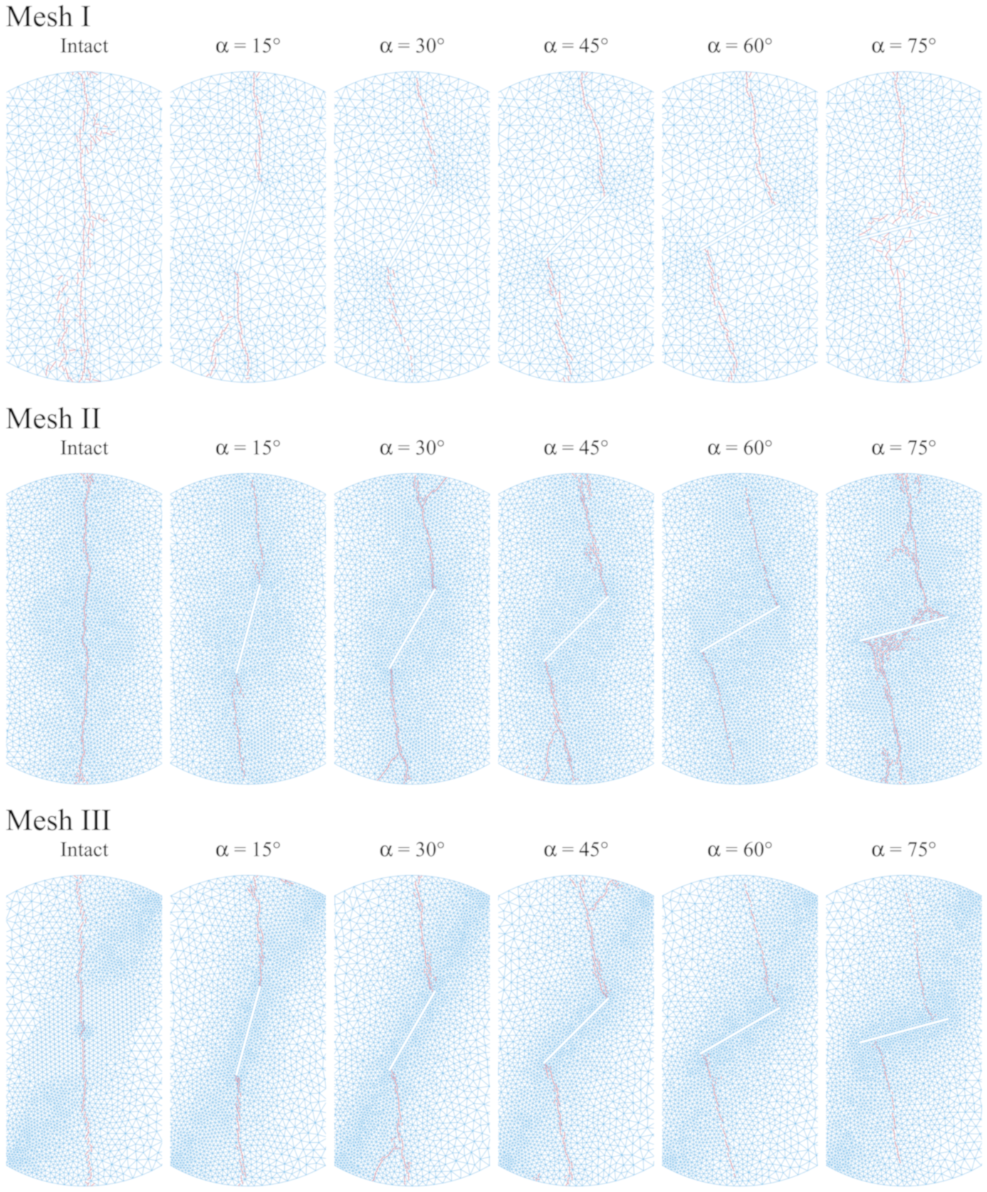
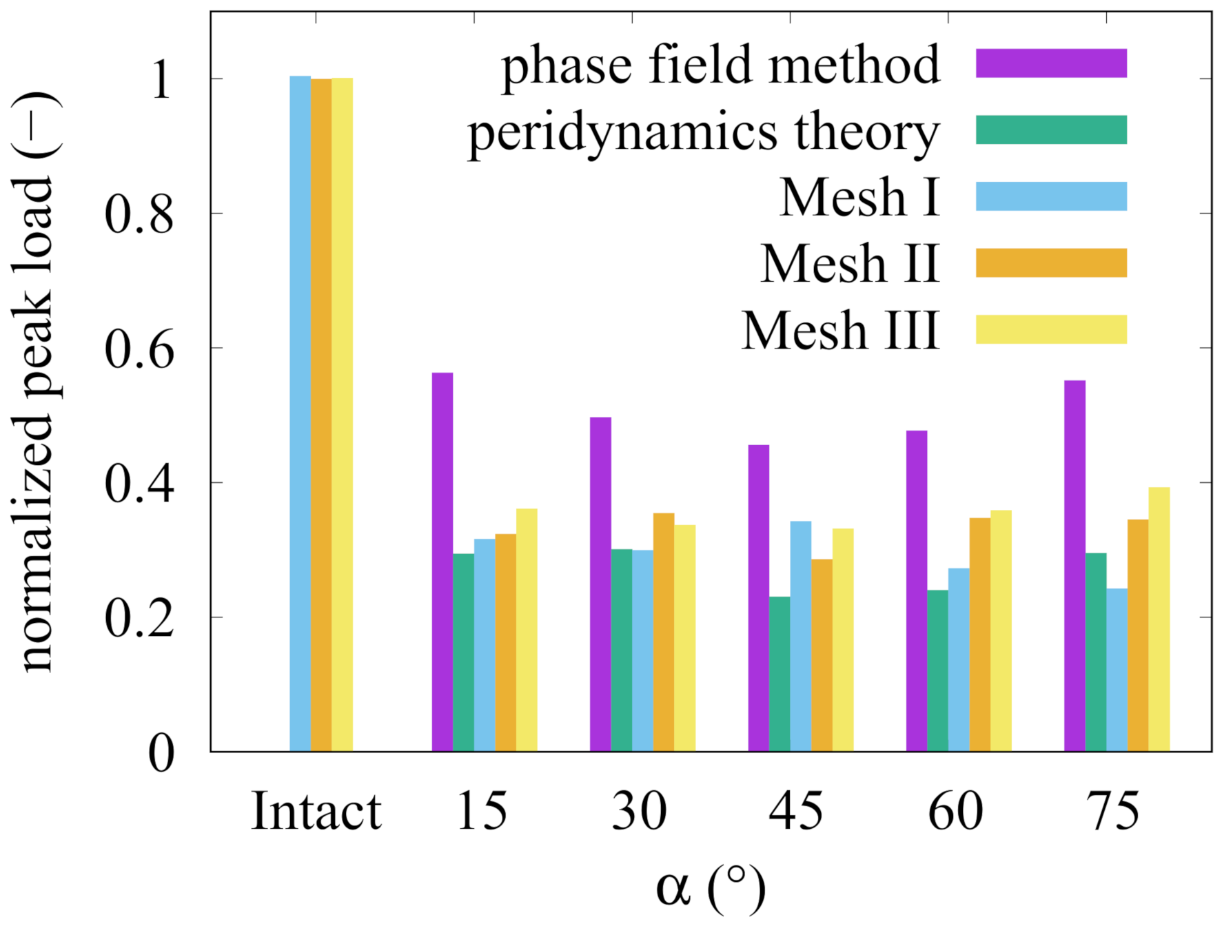
Brazilian disk tests with a single slot were experimentally investigated in [79]. The diameter of the disk is 10 cm. A slot with length 3 cm and width 0.1 cm is located in the middle of the disk, with inclination angle to the y-axis denoted as $\alpha$. The bottom 0.4 cm width of the disk is fixed when the top 0.4 cm width of the disk is vertically loaded. The elastic modulus E is 15 GPa, the Poisson’s ratio $\nu$ is 0.21, the fracture energy $G_f$ is 30 N/m, and the tensile strength $f_t$ is 3.81 MPa, see the model provided in [57]. The analytical peak load per unit thickness is $F_{peak}=\left(\pi D{f}_t\right)$/$2=$ 598.47 kN, which is used for obtaining the normalized peak loads. The numerically obtained crack paths are shown in Figure 3 and the normalized peak loads are shown in Figure 4 comparing the results provided in [80] (obtained by the phase field method) and [81] (by the bond-based peridynamics method). The results indicate the reliability of the CEM, which shows weak mesh dependency and agreeable results comparing to some other work.

3.2. Sandstone Containing Three Pre-Existing Fissures

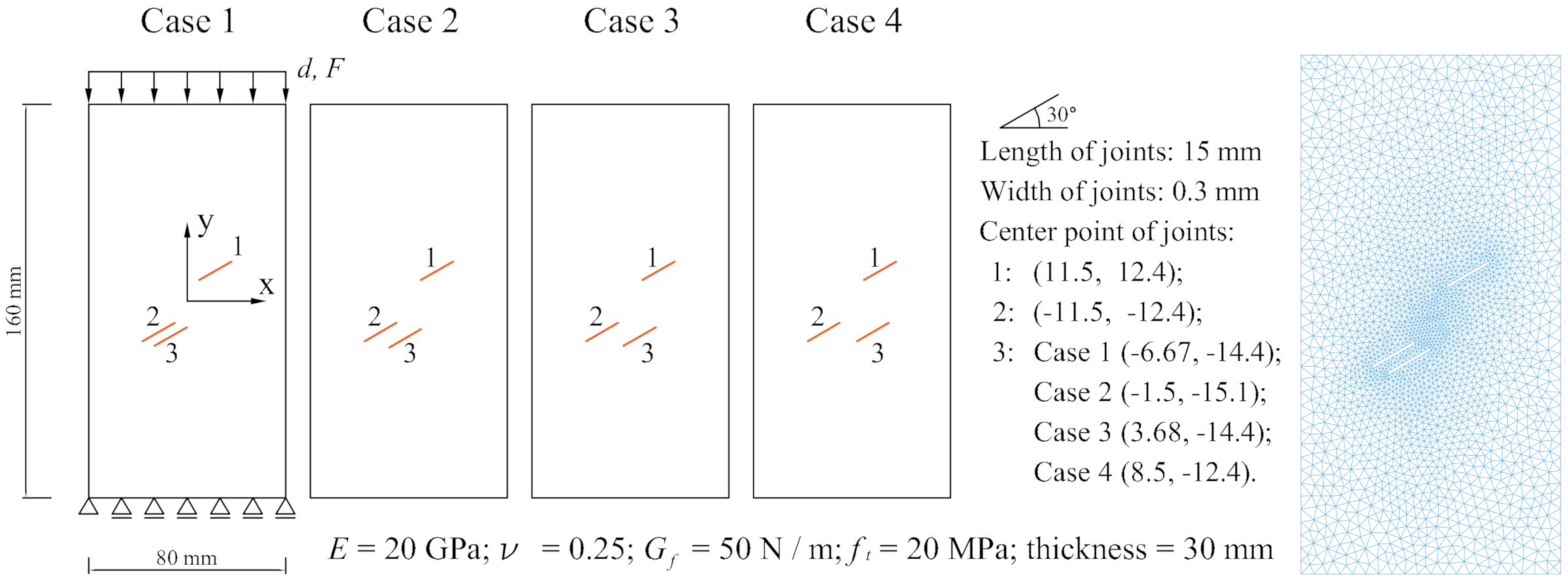
The second example concerns uniaxial compression tests for sandstone specimens with three fissures, which were experimentally studied in [82]. This example was numerically studied with the bond-based peridynamic model in [83] as a damage degree-based model. To the best of our knowledge, this example has not been numerically studied with a crack-opening-based model in published literature. The model, material, and discretization are shown in Figure 5. The meshes will change slightly with different setups for the fissures. Although the specimens are subjected to compression loading, they experience mainly tensile damage.

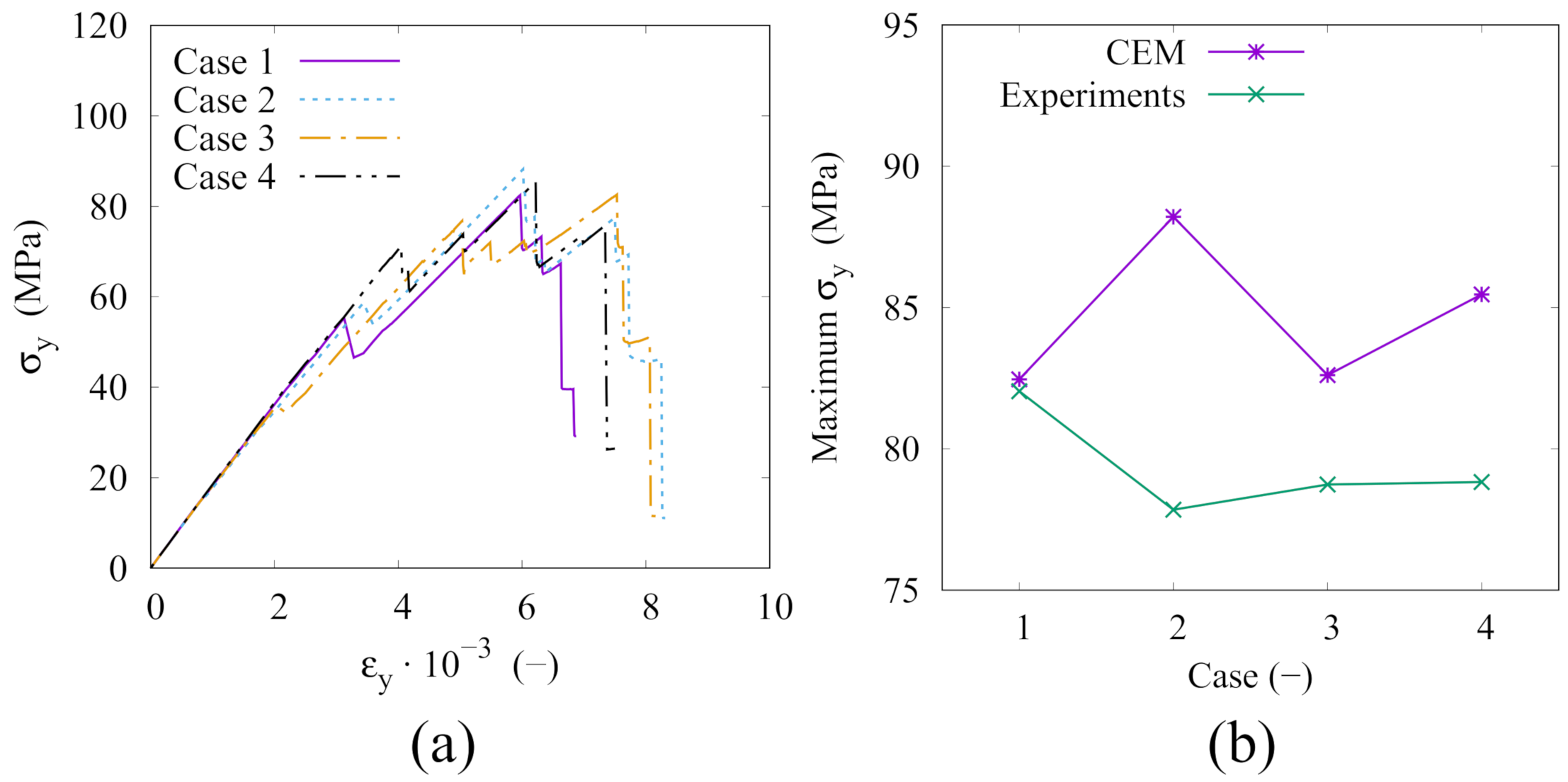
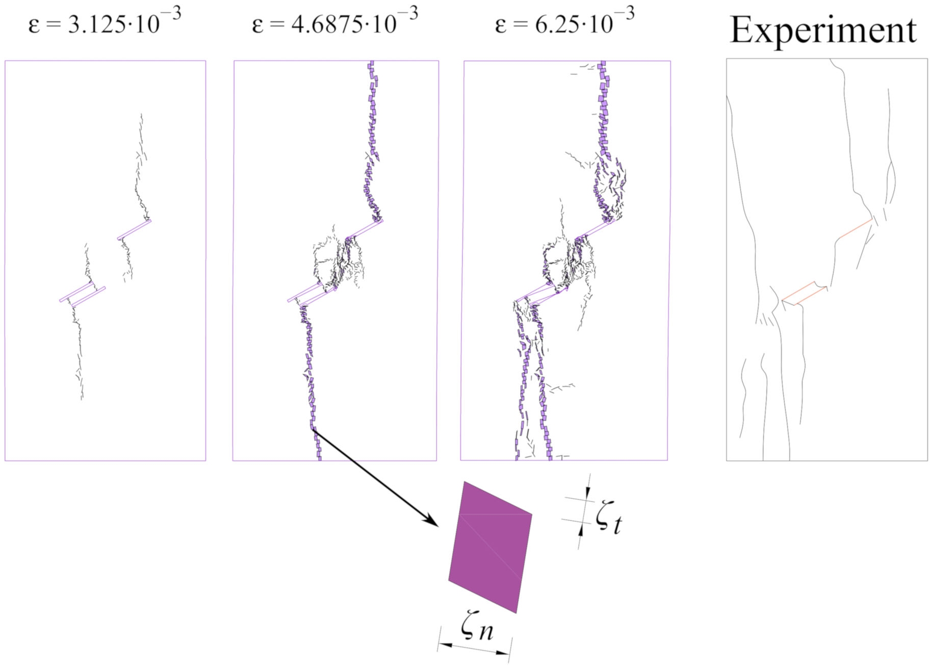
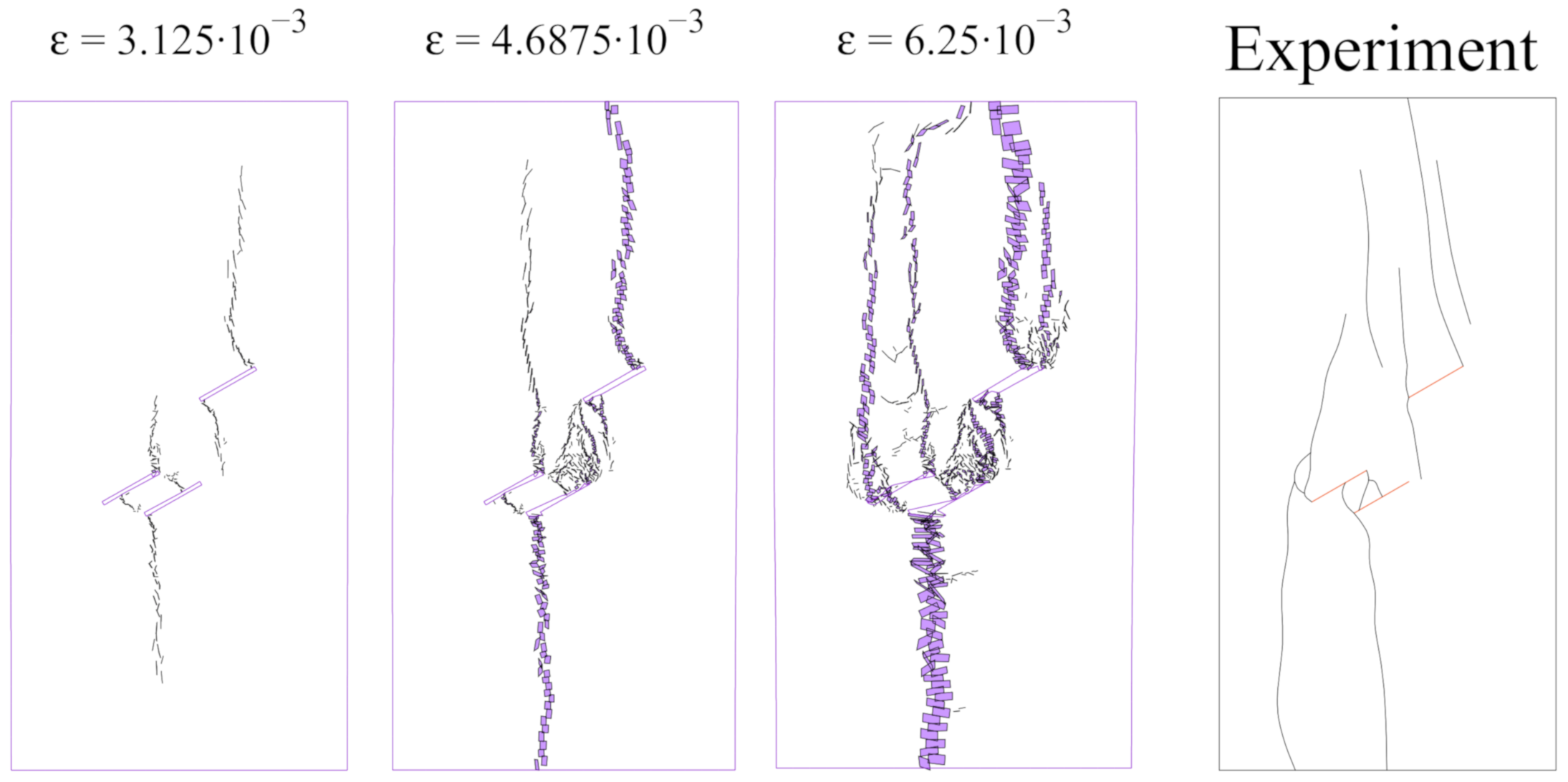
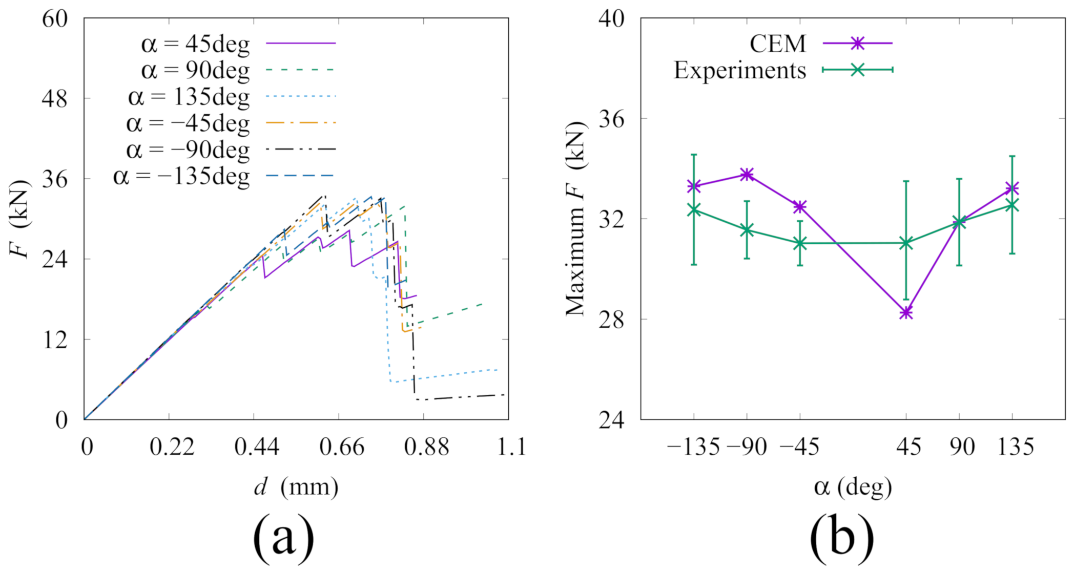
The force–displacement curves and the maximum vertical loads compared to the experimental results are shown in Figure 6. In the force–displacement curves, the oscillations correspond to the connecting of different fissures by propagating cracks. Furthermore, considering the maximum vertical loads, similar to the experimental results, we found that the position of fissure No. 3 has a limited influence on the maximum ${\sigma }_y$. The crack opening plots compared to the experimental results are shown in Figure 7, Figure 8, Figure 9 and Figure 10, where the small parallelograms represent the normal and shear crack opening, see Figure 7. The results indicate that the CEM is capable of simulating multiple crack propagations and connections among different fissures in the meanwhile the crack openings are obtained successfully.

3.3. 3D-Printed Materials with Two Intermittent Fissures

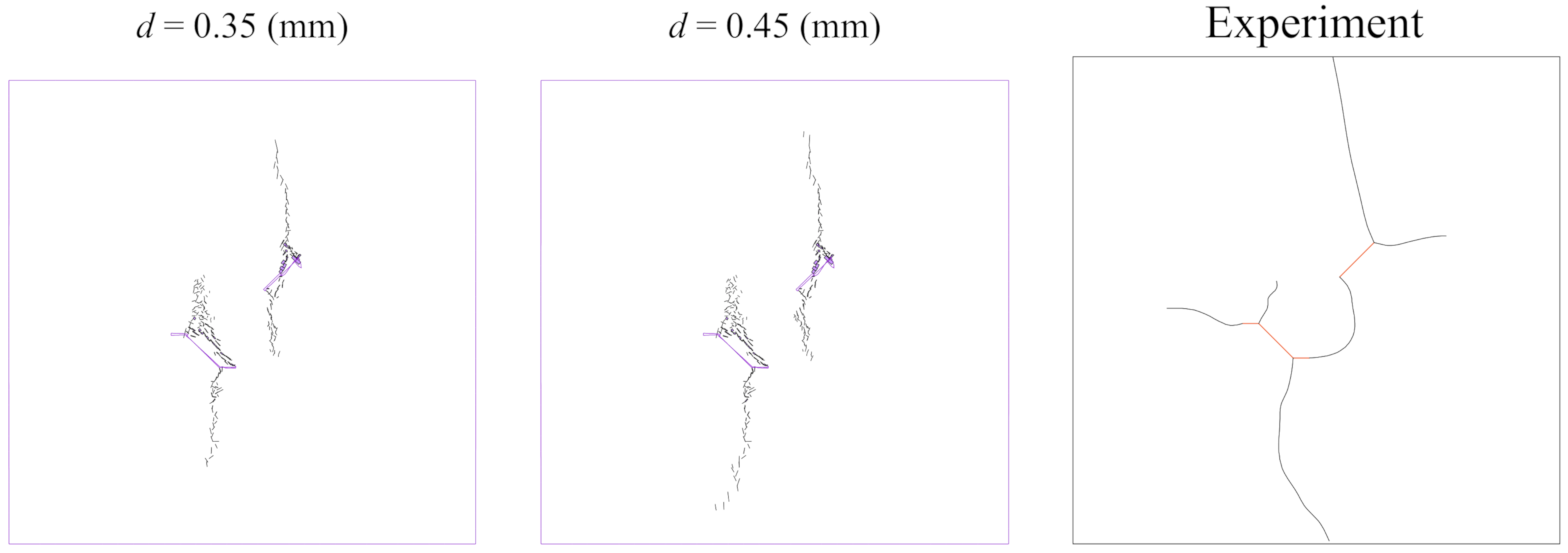
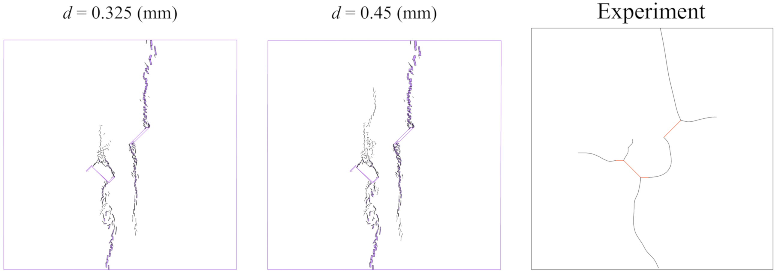
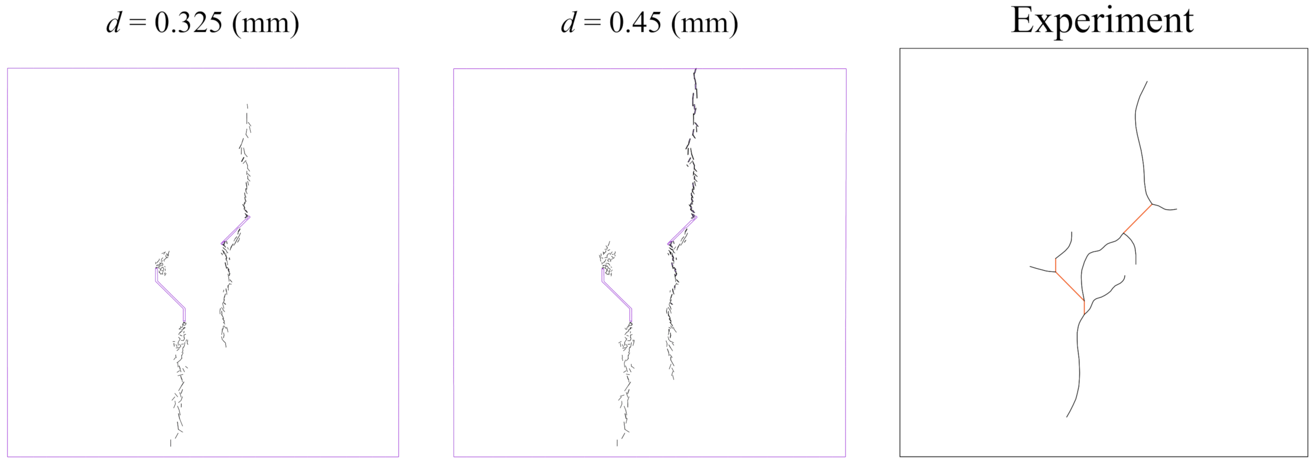
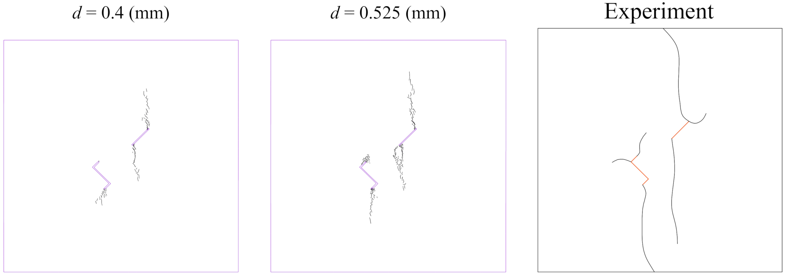
The third example concerns uniaxial compression tests on 3D-printed materials with two intermittent fissures, which were experimentally studied in [84]. The model, material, and discretization are shown in Figure 11, with fissures that are 0.3 mm in width. Only the elastic modulus, Poisson’s ratio, fracture energy, and uniaxial tensile strength are needed in our model.

The force–displacement curves and the maximum vertical loads compared to the experimental results are shown in Figure 12. Generally, the numerically obtained results are satisfactory. Parts of the crack opening plots compared to the experimental results are shown in Figure 13, Figure 14, Figure 15 and Figure 16. In most cases in the simulations, the two fissures are not connected by the propagating cracks, which does not accord well with the experimental results. We attribute the differences to two reasons: (i) the shearing damage is not accounted for in the present model, and (ii) the free horizontal boundary conditions on the top and bottom of the specimens cannot be ensured in the experimental investigations.

3.4. Rock-Like Materials with Nine Parallel Fissures

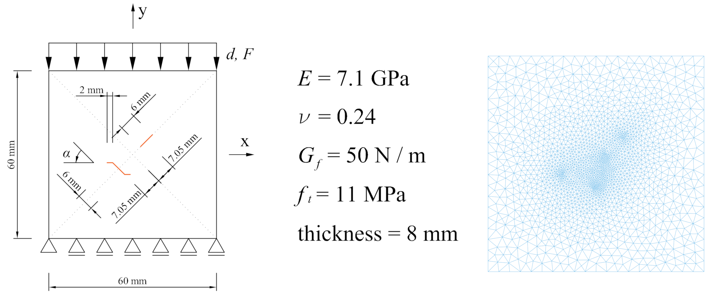
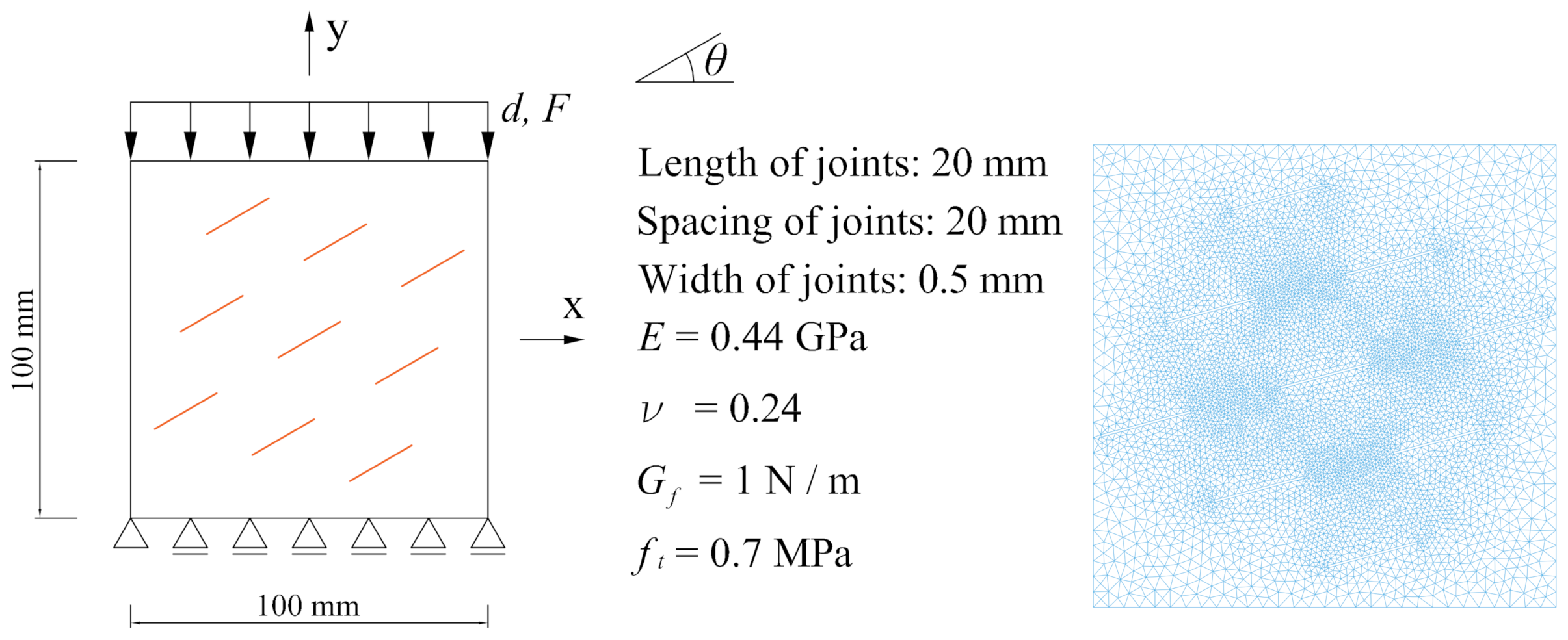
The last example concerns uniaxial compression tests of rock-like brittle materials with nine parallel fissures, which were experimentally studied in [85]. The model, material, and discretization are shown in Figure 17. Five cases with different values of $\theta$ are considered: $\theta ={15}^{\circ }$, $\theta ={30}^{\circ }$, $\theta ={45}^{\circ }$, $\theta ={60}^{\circ }$, and $\theta ={75}^{\circ }$.

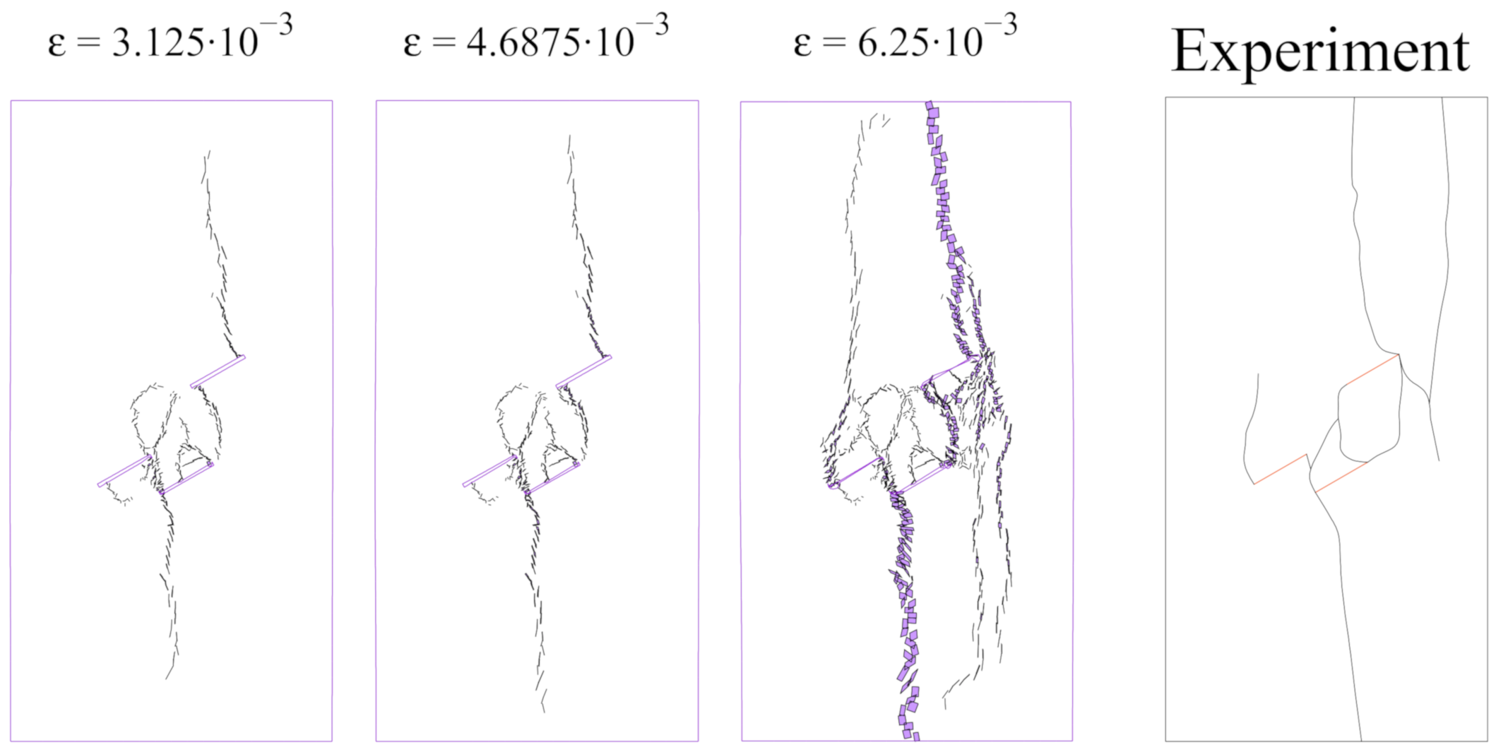
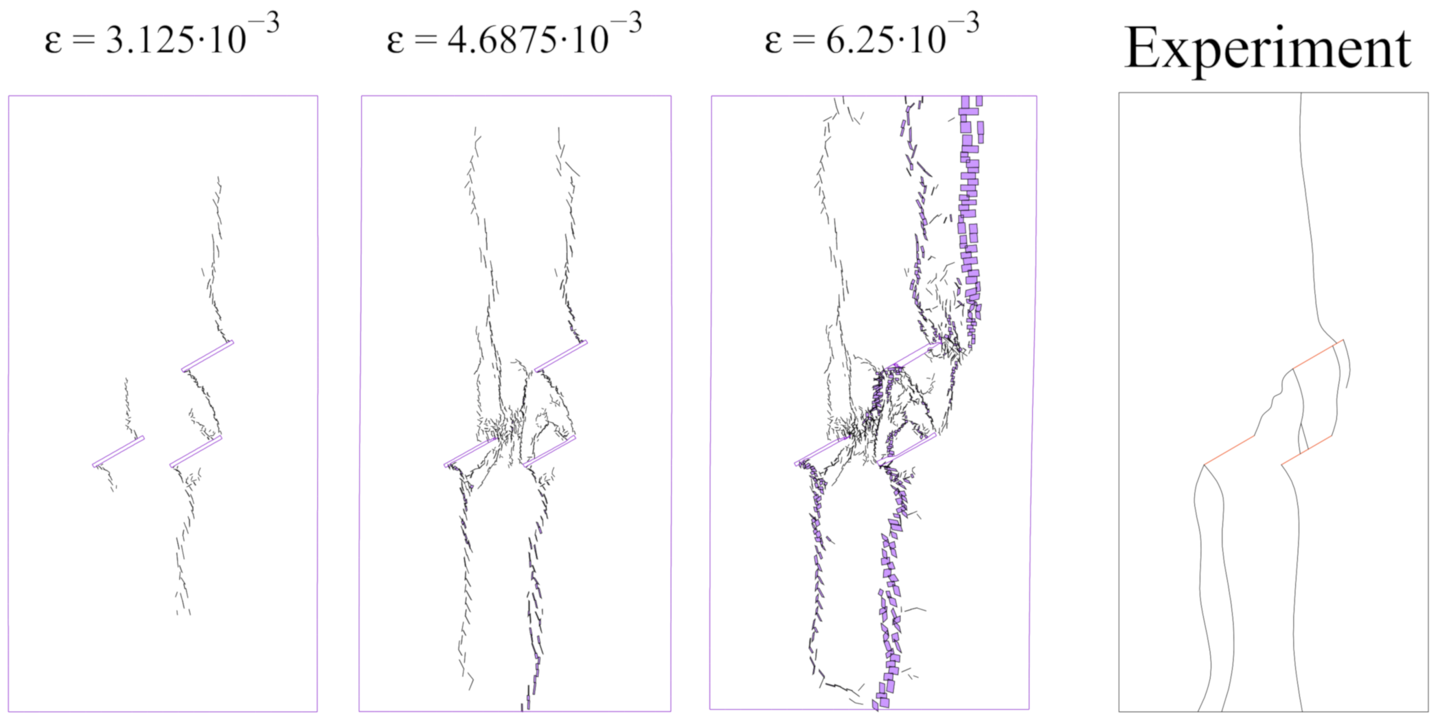
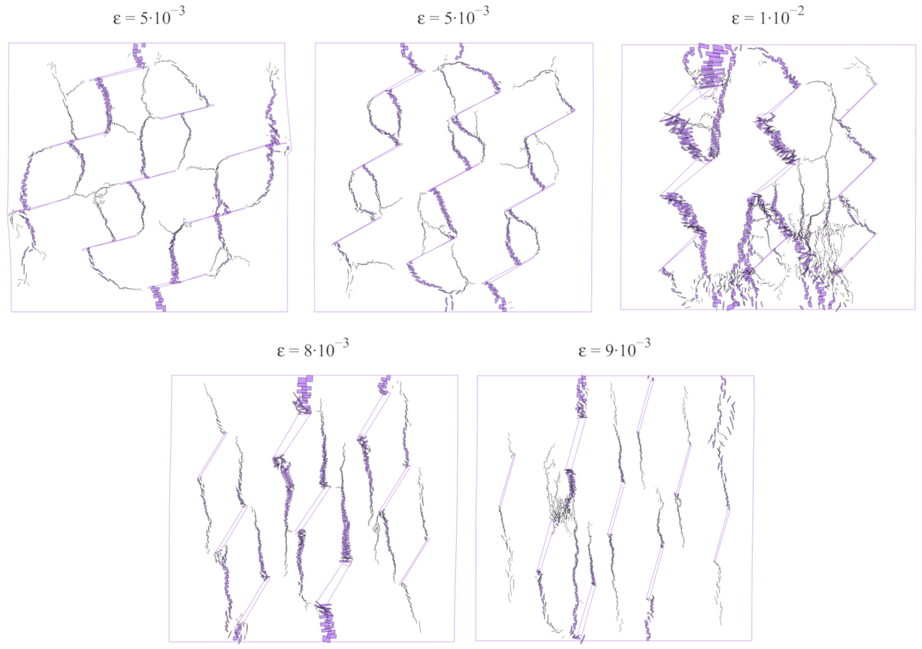
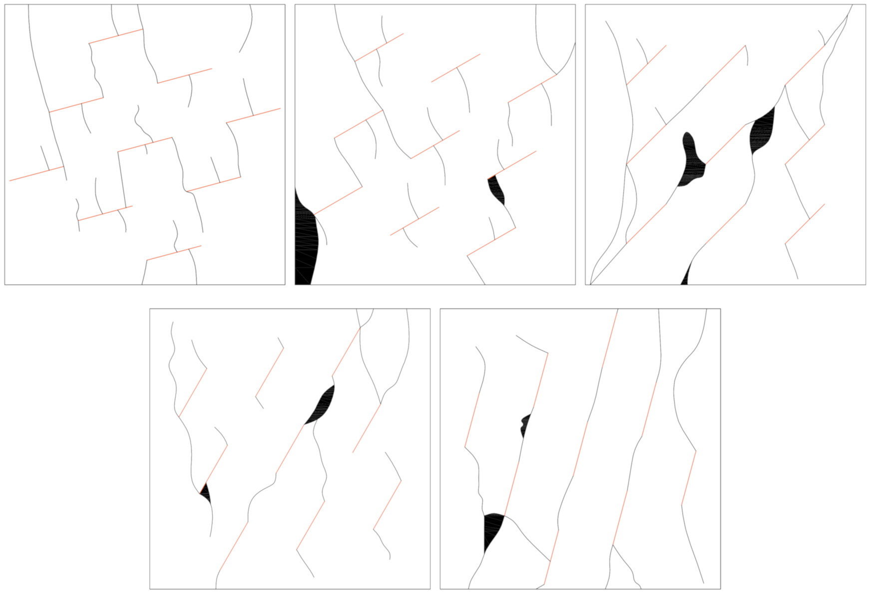
We compare only the numerically and experimentally obtained results of the crack opening (crack paths). The crack opening plots are shown in Figure 18. Comparing the experimental results shown in Figure 19, it can be found that the tensile-induced cracks are successfully captured by the CEM, including some branching and nucleation of the cracks. Especially for the cases with small values of $\theta$, tensile damage dominates. However, some drawbacks of our model are indicated:

• When the fissures are explicitly modeled, the contacts between the two surfaces of the fissures should be taken into account. When taking advantage of the CEM, implicit modeling of the fissures should be developed. In other words, the fissures should be treated as embedded cracks, where the closing of the cracks can be modeled more easily.
• With increasing $\theta$, the shearing damage becomes dominant. For shearing damage, the orientation of the shear bonds depends on the properties of the acoustic tensor [86,87]. The corresponding shearing damage criteria and model should be developed and implemented in the CEM.

4. Conclusions and Outlook

In this work, the damage processes of structures with fissures are analyzed with the cracking elements method (CEM). Uniaxial compression tests are considered, and the tensile damage model is used in this model. For such structures and loading conditions, cracks may propagate from the tips or other positions of the fissures. The cracks will either connect several fissures or propagate independently. Sometimes, new cracks may begin from unexpected positions. The results demonstrate the advantages of the CEM, which is capable of capturing both the initiation and propagation of cracks. On the other hand, some drawbacks of the present model are also revealed, indicating our future work with the CEM, including the implicit modeling of fissures and the implementation of shearing damage models. Furthermore, CEM can capture initiations and propagations of multiple cracks efficiently. Hence, it is supposed to be useful for predicting the damage behavior of the matrix–inclusion system such as composite materials. The corresponding studies are currently underway.

References

- De Borst, R.; Remmers, J.J.; Needleman, A.; Abellan, M.-A. Discrete vs smeared crack models for concrete fracture: Bridging the gap. Int. J. Numer. Anal. Methods Geomech. 2004, 28, 583–607. [Google Scholar] [CrossRef]
- Wu, J.-Y.; Qiu, J.-F.; Nguyen, V.P.; Mandal, T.K.; Zhuang, L.-J. Computational modeling of localized failure in solids: Xfem vs pf-czm. Comput. Methods Appl. Mech. Eng. 2019, 345, 618–643. [Google Scholar] [CrossRef]
- Zhang, Y.; Gao, Z.; Li, Y.; Zhuang, X. On the crack opening and energy dissipation in a continuum based disconnected crack model. Finite Elem. Anal. Des. 2020, 170, 103333. [Google Scholar] [CrossRef]
- Geers, M.; Borst, R.D.; Peerlings, R. Damage and crack modeling in single-edge and double-edge notched concrete beams. Eng. Fract. Mech. 2000, 65, 247–261. [Google Scholar] [CrossRef]
- Saloustros, S.; Pelà, L.; Cervera, M. A crack-tracking technique for localized cohesive–frictional damage. Eng. Fract. Mech. 2015, 150, 96–114. [Google Scholar] [CrossRef] [Green Version]
- Oliver, J.; Dias, I.; Huespe, A. Crack-path field and strain-injection techniques in computational modeling of propagating material failure. Comput. Methods Appl. Mech. Eng. 2014, 274, 289–348. [Google Scholar] [CrossRef] [Green Version]
- Saloustros, S.; Pelà, L.; Cervera, M.; Roca, P. Finite element modelling of internal and multiple localized cracks. Comput. Mech. 2017, 59, 299–316. [Google Scholar] [CrossRef] [Green Version]
- Armero, F.; Garikipati, K. An analysis of strong discontinuities in multiplicative finite strain plasticity and their relation with the numerical simulation of strain localization in solids. Int. J. Solids Struct. 1996, 33, 2863–2885. [Google Scholar] [CrossRef]
- Borja, R.I. Finite element simulation of strain localization with large deformation: Capturing strong discontinuity using a Petrov-Galerkin multiscale formulation. Comput. Methods Appl. Mech. Eng. 2002, 191, 2949–2978. [Google Scholar] [CrossRef] [Green Version]
- Giry, C.; Dufour, F.; Mazars, J. Stress-based nonlocal damage model. Int. J. Solids Struct. 2011, 48, 3431–3443. [Google Scholar] [CrossRef]
- Lorentz, E.; Badel, P. A new path-following constraint for strain-softening finite element simulations. Int. J. Numer. Methods Eng. 2004, 60, 499–526. [Google Scholar] [CrossRef]
- Silling, S. Reformulation of elasticity theory for discontinuities and long-range force. J. Mech. Phys. Solids 2000, 48, 175–209. [Google Scholar] [CrossRef] [Green Version]
- Silling, S.; Askari, E. A meshfree method based on the peridynamic model of solid mechanics. Comput. Struct. 2005, 83, 1526–1535. [Google Scholar] [CrossRef]
- Areias, P.; Reinoso, J.; Camanho, P.; Rabczuk, T. A constitutive-based element-by-element crack propagation algorithm with local mesh refinement. Comput. Mech. 2015, 56, 291–315. [Google Scholar] [CrossRef]
- Areias, P.; Rabczuk, T.; Dias-da-Costa, D. Element-wise fracture algorithm based on rotation of edges. Eng. Fract. Mech. 2013, 110, 113–137. [Google Scholar] [CrossRef]
- Yang, Z.; Deeks, A.; Hao, H. Transient dynamic fracture analysis using scaled boundary finite element method: A frequency-domain approach. Eng. Fract. Mech. 2007, 74, 669–687. [Google Scholar] [CrossRef]
- Ooi, E.; Shi, M.; Song, C.; Tin-Loi, F.; Yang, Z. Dynamic crack propagation simulation with scaled boundary polygon elements and automatic remeshing technique. Eng. Fract. Mech. 2013, 106, 1–21. [Google Scholar] [CrossRef]
- Song, J.-H.; Areias, P.; Belytschko, T. A method for dynamic crack and shear band propagation with phantom nodes. Int. J. Numer. Methods Eng. 2006, 67, 868–893. [Google Scholar] [CrossRef]
- Belytschko, T.; Chen, H.; Xu, J.; Zi, G. Dynamic crack propagation based on loss of hyperbolicity with a new discontinuous enrichment. Int. J. Numer. Methods Eng. 2003, 58, 1873–1905. [Google Scholar] [CrossRef]
- Wu, Z.; Xu, X.; Liu, Q.; Yang, Y. A zero-thickness cohesive element-based numerical manifold method for rock mechanical behavior with micro-voronoi grains. Eng. Anal. Bound. Elem. 2018, 96, 94–108. [Google Scholar] [CrossRef]
- Wu, J.; Cai, Y. A partition of unity formulation referring to the nmm for multiple intersecting crack analysis. Theor. Appl. Fract. Mech. 2014, 72, 28–36. [Google Scholar] [CrossRef]
- Wu, J.-Y.; Li, F.-B.; Xu, S.-L. Extended embedded finite elements with continuous displacement jumps for the modeling of localized failure in solids. Comput. Methods Appl. Mech. Eng. 2015, 285, 346–378. [Google Scholar] [CrossRef]
- Armero, F.; Linder, C. New finite elements with embedded strong discontinuities in the finite deformation range. Comput. Methods Appl. Mech. Eng. 2008, 197, 3138–3170. [Google Scholar] [CrossRef]
- Rabczuk, T.; Belytschko, T. Adaptivity for structured meshfree particle methods in 2D and 3D. Int. J. Numer. Methods Eng. 2005, 63, 1559–1582. [Google Scholar] [CrossRef]
- Zhuang, X.; Augarde, C.; Mathisen, K. Fracture modeling using meshless methods and level sets in 3D: Framework and modeling. Int. J. Numer. Methods Eng. 2012, 92, 969–998. [Google Scholar] [CrossRef]
- Zhuang, X.; Augarde, C.; Bordas, S. Accurate fracture modelling using meshless methods, the visibility criterion and level sets: Formulation and 2D modelling. Int. J. Numer. Methods Eng. 2011, 86, 249–268. [Google Scholar] [CrossRef]
- Areias, P.; Rabczuk, T. Steiner-point free edge cutting of tetrahedral meshes with applications in fracture. Finite Elem. Anal. Des. 2017, 132, 27–41. [Google Scholar] [CrossRef] [Green Version]
- Areias, P.; Msekh, M.; Rabczuk, T. Damage and fracture algorithm using the screened Poisson equation and local remeshing. Eng. Fract. Mech. 2016, 158, 116–143. [Google Scholar] [CrossRef]
- Wu, J.-Y.; Li, F.-B. An improved stable XFEM (Is-XFEM) with a novel enrichment function for the computational modeling of cohesive cracks. Comput. Methods Appl. Mech. Eng. 2015, 295, 77–107. [Google Scholar] [CrossRef]
- Chau-Dinh, T.; Zi, G.; Lee, P.-S.; Rabczuk, T.; Song, J.-H. Phantom-node method for shell models with arbitrary cracks. Comput. Struct. 2012, 92–93, 242–246. [Google Scholar] [CrossRef]
- Wang, Y.; Waisman, H.; Harari, I. Direct evaluation of stress intensity factors for curved cracks using Irwin’s integral and XFEM with high-order enrichment functions. Int. J. Numer. Methods Eng. 2017, 112, 629–654. [Google Scholar] [CrossRef]
- Zheng, H.; Xu, D. New strategies for some issues of numerical manifold method in simulation of crack propagation. Int. J. Numer. Methods Eng. 2014, 97, 986–1010. [Google Scholar] [CrossRef]
- Zheng, H.; Liu, F.; Du, X. Complementarity problem arising from static growth of multiple cracks and mls-based numerical manifold method. Comput. Methods Appl. Mech. Eng. 2015, 295, 150–171. [Google Scholar] [CrossRef]
- Wu, Z.; Ngai, L.; Wong, Y. Frictional crack initiation and propagation analysis using the numerical manifold method. Comput. Geotech. 2012, 39, 38–53. [Google Scholar] [CrossRef]
- Wu, Z.; Fan, L.; Liu, Q.; Ma, G. Micro-mechanical modeling of the macro-mechanical response and fracture behavior of rock using the numerical manifold method. Eng. Geol. 2017, 225, 49–60. [Google Scholar] [CrossRef]
- Wu, J.-Y. Nguyen, V.P. A length scale insensitive phase-field damage model for brittle fracture. J. Mech. Phys. Solids 2018, 119, 20–42. [Google Scholar] [CrossRef]
- Wu, J.-Y. Robust numerical implementation of non-standard phase-field damage models for failure in solids. Comput. Methods Appl. Mech. Eng. 2018, 340, 767–797. [Google Scholar] [CrossRef]
- Wu, J.-Y. A unified phase-field theory for the mechanics of damage and quasi-brittle failure. J. Mech. Phys. Solids 2017, 103, 72–99. [Google Scholar] [CrossRef]
- Zhou, S.; Zhuang, X.; Zhu, H.; Rabczuk, T. Phase field modelling of crack propagation, branching and coalescence in rocks. Theor. Appl. Fract. Mech. 2018, 96, 174–192. [Google Scholar] [CrossRef] [Green Version]
- Cervera, M.; Chiumenti, M.; Codina, R. Mixed stabilized finite element methods in nonlinear solid mechanics: Part I: Formulation. Comput. Methods Appl. Mech. Eng. 2010, 199, 2559–2570. [Google Scholar] [CrossRef]
- Cervera, M.; Chiumenti, M.; Codina, R. Mixed stabilized finite element methods in nonlinear solid mechanics: Part II: Strain localization. Comput. Methods Appl. Mech. Eng. 2010, 199, 2571–2589. [Google Scholar] [CrossRef]
- Cervera, M.; Chiumenti, M.; Benedetti, L.; Codina, R. Mixed stabilized finite element methods in nonlinear solid mechanics. Part III: Compressible and incompressible plasticity. Comput. Methods Appl. Mech. Eng. 2015, 285, 752–775. [Google Scholar] [CrossRef] [Green Version]
- Cervera, M.; Chiumenti, M.; Codina, R. Mesh objective modeling of cracks using continuous linear strain and displacement interpolations. Int. J. Numer. Methods Eng. 2011, 87, 962–987. [Google Scholar] [CrossRef]
- Nikolić, M.; Karavelić, E.; Ibrahimbegovic, A.; Mišćevixcx, P. Lattice element models and their peculiarities. Arch. Comput. Methods Eng. 2018, 25, 753–784. [Google Scholar] [CrossRef] [Green Version]
- Jiang, C.; Zhao, G.-F.; Khalili, N. On crack propagation in brittle material using the distinct lattice spring model. Int. J. Solids Struct. 2017, 118–119, 41–57. [Google Scholar] [CrossRef]
- Kosteski, L.E.; Iturrioz, I.; Cisilino, A.P.; D’ambra, R.B.; Pettarin, V.; Fasce, L.; Frontini, P. A lattice discrete element method to model the falling-weight impact test of PMMA specimens. Int. J. Impact Eng. 2016, 87, 120–131. [Google Scholar] [CrossRef]
- Zhao, G.-F. Developing a four-dimensional lattice spring model for mechanical responses of solids. Comput. Methods Appl. Mech. Eng. 2017, 315, 881–895. [Google Scholar] [CrossRef]
- Ren, H.; Zhuang, X.; Cai, Y.; Rabczuk, T. Dual-horizon peridynamics. Int. J. Numer. Methods Eng. 2016, 108, 1451–1476. [Google Scholar] [CrossRef] [Green Version]
- Ren, H.; Zhuang, X.; Rabczuk, T. Dual-horizon peridynamics: A stable solution to varying horizons. Comput. Methods Appl. Mech. Eng. 2017, 318, 762–782. [Google Scholar] [CrossRef] [Green Version]
- Diana, V.; Casolo, S. A bond-based micropolar peridynamic model with shear deformability: Elasticity, failure properties and initial yield domains. Int. J. Solids Struct. 2019, 160, 201–231. [Google Scholar] [CrossRef]
- Ren, H.; Zhuang, X.; Rabczuk, T. Nonlocal operator method with numerical integration for gradient solid. Comput. Struct. 2020, 233, 106235. [Google Scholar] [CrossRef]
- Saloustros, S.; Cervera, M.; Pelà, L. Challenges, tools and applications of tracking algorithms in the numerical modelling of cracks in concrete and masonry structures. Arch. Comput. Methods Eng. 2019, 26, 961–1005. [Google Scholar] [CrossRef] [Green Version]
- Alsahly, A.; Callari, C.; Meschke, G. An algorithm based on incompatible modes for the global tracking of strong discontinuities in shear localization analyses. Comput. Methods Appl. Mech. Eng. 2018, 330, 33–63. [Google Scholar] [CrossRef]
- Zhang, Y.; Zhuang, X. Cracking elements: A self-propagating strong discontinuity embedded approach for quasi-brittle fracture. Finite Elem. Anal. Des. 2018, 144, 84–100. [Google Scholar] [CrossRef]
- Zhang, Y.; Zhuang, X. Cracking elements method for dynamic brittle fracture. Theor. Appl. Fract. Mech. 2019, 102, 1–9. [Google Scholar] [CrossRef]
- Zhang, Y.; Mang, H.A. Global cracking elements: A novel tool for Galerkin-based approaches simulating quasi-brittle fracture. Int. J. Numer. Methods Eng. 2020, 121, 2462–2480. [Google Scholar] [CrossRef]
- Mu, L.; Zhang, Y. Cracking elements method with 6-node triangular element. Finite Elem. Anal. Des. 2020, 177, 103421. [Google Scholar] [CrossRef]
- Dias-da-Costa, D.; Alfaiate, J.; Sluys, L.; Areias, P.; Júlio, E. An embedded formulation with conforming finite elements to capture strong discontinuities. Int. J. Numer. Methods Eng. 2012, 93, 224–244. [Google Scholar] [CrossRef]
- Cervera, M.; Wu, J.-Y.; Chiumenti, M.; Kim, S. Strain localization analysis of Hill’s orthotropic elastoplasticity: Analytical results and numerical verification. Comput. Mech. 2020, 65, 533–554. [Google Scholar] [CrossRef]
- Nikolić, M.; Do, X.N.; Ibrahimbegovic, A.; Nikolić, Ž. Crack propagation in dynamics by embedded strong discontinuity approach: Enhanced solid versus discrete lattice model. Comput. Methods Appl. Mech. Eng. 2018, 340, 480–499. [Google Scholar] [CrossRef] [Green Version]
- Lloberas-Valls, O.; Huerta, A.; Oliver, J.; Dias, I. Strain injection techniques in dynamic fracture modeling. Comput. Methods Appl. Mech. Eng. 2016, 308, 499–534. [Google Scholar] [CrossRef] [Green Version]
- Zhang, Y.; Lackner, R.; Zeiml, M.; Mang, H. Strong discontinuity embedded approach with standard SOS formulation: Element formulation, energy-based crack-tracking strategy, and validations. Comput. Methods Appl. Mech. Eng. 2015, 287, 335–366. [Google Scholar] [CrossRef]
- Rabczuk, T.; Bordas, S.; Zi, G. On three-dimensional modelling of crack growth using partition of unity methods. Comput. Struct. 2010, 88, 1391–1411. [Google Scholar] [CrossRef]
- Rabczuk, T.; Belytschko, T. Cracking particles: A simplified meshfree method for arbitrary evolving cracks. Int. J. Numer. Methods Eng. 2004, 61, 2316–2343. [Google Scholar] [CrossRef]
- Rabczuk, T.; Belytschko, T. A three-dimensional large deformation meshfree method for arbitrary evolving cracks. Comput. Methods Appl. Mech. Eng. 2007, 196, 2777–2799. [Google Scholar] [CrossRef] [Green Version]
- Rabczuk, T.; Zi, G.; Bordas, S.; Nguyen-Xuan, H. A simple and robust three-dimensional cracking-particle method without enrichment. Comput. Methods Appl. Mech. Eng. 2010, 199, 2437–2455. [Google Scholar] [CrossRef]
- Suárez, F.; Gálvez, J.; Cendón, D. A material model to reproduce mixed-mode fracture in concrete. Fatigue Fract. Eng. Mater. Struct. 2019, 42, 223–238. [Google Scholar] [CrossRef] [Green Version]
- Meschke, G.; Dumstorff, P. Energy-based modeling of cohesive and cohesionless cracks via X-FEM. Comput. Methods Appl. Mech. Eng. 2007, 196, 2338–2357. [Google Scholar] [CrossRef]
- Belytschko, T.; Organ, D.; Gerlach, C. Element-free Galerkin methods for dynamic fracture in concrete. Comput. Methods Appl. Mech. Eng. 2000, 187, 385–399. [Google Scholar] [CrossRef]
- Zhang, Y.; Zhuang, X. A softening-healing law for self-healing quasi-brittle materials: Analyzing with strong discontinuity embedded approach. Eng. Fract. Mech. 2018, 192, 290–306. [Google Scholar] [CrossRef] [Green Version]
- Mosler, J.; Meschke, G. 3D modelling of strong discontinuities in elastoplastic solids: Fixed and rotating localization formulations. Int. J. Numer. Methods Eng. 2003, 57, 1553–1576. [Google Scholar] [CrossRef]
- Mosler, J.; Bruhns, O. A 3D anisotropic elastoplastic-damage model using discontinuous displacement fields. Int. J. Numer. Methods Eng. 2004, 60, 923–948. [Google Scholar] [CrossRef]
- Simo, J.; Rifai, S. A class of mixed assumed strain methods and the method of incompatible modes. Int. J. Numer. Methods Eng. 1990, 29, 1595–1638. [Google Scholar] [CrossRef]
- Simo, J.; Oliver, J.; Armero, F. An analysis of strong discontinuities induced by strain-softening in rate-independent inelastic solids. Comput. Mech. 1993, 12, 277–296. [Google Scholar] [CrossRef]
- Simo, J.; Armero, F. Geometrically nonlinear enhanced strain mixed methods and the method of incompatible modes. Int. J. Numer. Methods Eng. 1992, 33, 1413–1449. [Google Scholar] [CrossRef]
- Helnwein, P. Some remarks on the compressed matrix representation of symmetric second-order and fourth-order tensors. Comput. Methods Appl. Mech. Eng. 2001, 190, 2753–2770. [Google Scholar] [CrossRef]
- Oliver, J. A consistent characteristic length for smeared cracking models. Int. J. Numer. Methods Eng. 1989, 28, 461–474. [Google Scholar] [CrossRef]
- Cervera, M.; Chiumenti, M. Smeared crack approach: Back to the original track. Int. J. Numer. Anal. Methods Geomech. 2006, 30, 1173–1199. [Google Scholar] [CrossRef]
- Haeri, H.; Shahriar, K.; Marji, M.F.; Moarefvand, P. Experimental and numerical study of crack propagation and coalescence in pre-cracked rock-like disks. Int. J. Rock Mech. Min. Sci. 2014, 67, 20–28. [Google Scholar] [CrossRef]
- Zhou, S.-W.; Xia, C.-C. Propagation and coalescence of quasi-static cracks in Brazilian disks: An insight from a phase field model. Acta Geotech. 2019, 14, 1195–1214. [Google Scholar] [CrossRef]
- Zhou, X.-P.; Wang, Y.-T. Numerical simulation of crack propagation and coalescence in pre-cracked rock-like Brazilian disks using the non-ordinary state-based peridynamics. Int. J. Rock Mech. Min. Sci. 2016, 89, 235–249. [Google Scholar] [CrossRef]
- Yang, S.-Q. Study of strength failure and crack coalescence behavior of sandstone containing three pre-existing fissures (in Chinese). Rock Soil Mech. (Yan Xue) 2013, 34, 31–39. [Google Scholar]
- Zhu, Q.; Ni, T.; Zhao, L. Shuangshuang, Y.; Simulations of crack propagation in rock-like materials using peridynamic method (in Chinese). Chin. J. Rock Mech. Eng. (Yan Shi Xue Gong Cheng Xue Bao) 2016, 35, 3507–3515. [Google Scholar]
- Zhang, D.; Dong, Q. Fracturing and damage of 3d-Printed materials with two intermittent fissures under compression. Materials 2020, 13, 1607. [Google Scholar] [CrossRef] [PubMed] [Green Version]
- Su, H.-J.; Jing, H.-W.; Zhao, H.-H.; Zhang, M.-L.; Yin, Q. Strength and fracture characteristic of rock mass containing parallel fissures (in Chinese). Eng. Mech. (Gong Cheng Xue) 2015, 32, 192–207. [Google Scholar]
- Pivonka, P.; Lackner, R.; Mang, H.A. Shapes of loading surfaces of concrete models and their influence on the peak load and failure mode in structural analyses. Int. J. Eng. Sci. 2003, 41, 1649–1665. [Google Scholar] [CrossRef]
- Rabczuk, T.; Samaniego, E. Discontinuous modelling of shear bands using adaptive meshfree methods. Comput. Methods Appl. Mech. Eng. 2008, 197, 641–658. [Google Scholar] [CrossRef] [Green Version]
Figure 1.
The basic of the cohesive zone model (redrawn based on the figure provided in [67]).
Figure 2.
Relationships between , and of Q8 and T6.
Figure 3.
Brazilian disk tests: crack paths regarding different inclined angle and meshes.
Figure 4.
Brazilian disk tests: normalized peak loads compared to the results published in [80] (obtained by the phase field method) and [81] (by the bond-based peridynamics method).