Wave Planning for Cart Picking in a Randomized Storage Warehouse

Abstract

Randomized storage strategy is known as a best practice for storing books of an online bookstore, it simplifies the order picking strategy as to retrieve books in purchase orders from closest locations of the warehouse. However, to be more responsive to customers, many distribution centers have adopted a just-in-time strategy leading to various value-added activities such as kitting, labelling, product or order assembly, customized packaging, or palletization, all of which must be scheduled and integrated in the order-picking process, and this is known as wave planning. In this study, we present a wave planning mathematical model by simultaneously consider: (1) time window from master of schedule (MOS), (2) random storage stock-keeping units (SKUs), and (3) picker-to-order. A conceptual simulation, along with a simplified example for the proposed wave planning algorithm, has been examined to demonstrate the merits of the idea. The result shows the wave planning module can improve the waiting time for truck loading of packages significantly and can reduce the time that packages are heaping in buffer area. The main contribution of this research is to develop a mixed integer programming model that helps the bookseller to generate optimal wave picking lists for a given time window.

1. Introduction

1.1. The Purpose of Randomized Storage Warehouse

Randomized storage is a storage assignment strategy which determines how an item can be stored in any empty location in a warehouse. One stock keeping unit (SKU) could therefore be stored in several different locations, and the advantage of this strategy is to exploit spaces more efficiently. Randomized storage strategy is especially suitable for storing books of an online bookstore. Customers like to make multiple purchases in a single order to eliminate shipping cost. By using a randomized storage warehouse for an online bookstore, the order picking strategy can be simplified as to retrieve books in purchase orders from closest locations of the warehouse.

1.2. The Importance of Order Picking for a Warehouse and the Type of Order Picking

Warehouse order picking is a simple concept, but in practice, the picking process can be complicated. Warehouse order picking refers to the necessary labor and parts involved in pulling items out of inventory to fulfill customer orders [1]. This process may sound like the simplest aspect of a business, but when one deals with numbers and realizes that in any given distribution center, order picking counts as the most time-consuming operation and an average of 55% of operating costs. A well-thought-out warehouse will soon find out these ineffective systems may prevent them from further innovation. For a business to develop a warehouse order picking strategy to meet the demand shifts of the future, the emphasizes on speediness, accuracy, and organization should always be bear in mind.

There are many types of order picking. Some of the order pickings are classified by the customer order handling policies, some are classified by equipment used by pickers, some are classified by warehousing areas, and the others are classified by materials handling equipment. For example, discrete order picking and batch picking are those classified by the customer order handling policies; cart picking, radio frequency (RF) picking, voice picking, tote picking, and put to store are those classified by equipment used by pickers; pick and pass or zone order picking are classified by warehousing areas; and full pallet picking and materials handling equipment assisted picking are those classified by materials handling equipment used. Discrete picking is when a picker goes through one order at a time, grabbing an item line by line before moving onto the next order. It is the simplest of all order picking methods and can also be one of the most accurate. Discrete order picking with a RF scanner or voice assistant device helps to streamline the process and increase accuracy. Cases where discrete order picking can be ideal include (1) when a warehouse has a small staff, (2) when orders are for multiple items, and (3) when the items ordered are very large. Batch picking is the process of collecting inventory for identical orders at once, rather than picking items one order at a time or picking orders with different SKUs and quantities consecutively. Batch picking focused on less walking and faster order processing. It is particularly good for warehouses that stock small items. In pick and pack operations, instead of batching the items into an order tote, you can pick orders directly into a shipping tote. Put-to-store is often used with picking carts to facilitate batch picking of multiple orders in one pass. It is ideal for retail store replenishment. It also optimizes cross-docking operations where a percentage of full case quantities are broken down to store level cartons. Zone order picking is a picking technique in which warehouses have been sectioned into several zones, and pickers have been assigned to each zone. Pickers pick all of the items from a customer order that are located in their zone and then passing the order on to the next zone, so that zone order picking is also called pick and pass order picking. Zone picking is particularly useful in large warehouses that deal with a high number of SKUs. Because each picker is assigned to a designated area, it allows pickers to gain deep familiarity with their assigned zones and the SKUs stored there, which can increase picking speed and reduce errors.

In this paper, we suggest looking at an order picking problem from forms and workflow of a warehouse management system (WMS) perspective. This would help one to tackle (i.e., finding out the considering factors/attributes) an order picking planning problem.

From information technology perspective (i.e., data and workflow), the inputs of a WMS are customer orders and pre-packaged stock keeping units [2]. For control and management purposes, the most important attributes in customer orders are what SKU (or item), how many quantities, and where (location) to deliver for each customer order (illustrated as (I Q L) in Figure 1), and in pre-packaged SKUs what are the SKUs and how many quantities are for pre-packaging (illustrated as (I Q) in Figure 1). A master order schedule (MOS) is another form recording what SKU and how many quantities are going to process for delivering. MOS is more like a filter that filters what customer orders and/or pre-packaged SKU are going to process based on similarity of delivery routing [3] or similarity of in-coming customer orders’ time windows [3,4]. The important attributes in MOS are what SKU, how many quantities, and when to load into what routing trucks (illustrated as (I Q R) in Figure 1).

By considering SKU storage locations, customer orders in MOS are further batched or split [5,6] based on similarity of their SKUs’ storage locations. The major concerns of batching or splitting are what SKU, how many quantities, and where storage (illustrated as (I Q S) in Figure 1). Batched or split order picking calls for managers to assess current orders for popularity and place them into batches by their SKU. From there, pickers are in the best location of the warehouse to get orders fulfilled as quickly as possible. Batch picking works especially well for e-commerce businesses with somewhat predictable ordering trends, like those specializing in food and apparel. There are lots of order picking policies proposed at this research field, discrete picking, zone picking, and wave picking [5,7]. Discrete picking policy is when a picker picks items of multiple orders by batching during a single trip. Zone picking policy divides the picking area into a few subzones and the dedicated picker will pick items by splitting in that subzone only. The main research topic is the number of subzones and pickers. Wave picking is used if orders by splitting and/or batching for a common destination or common truck loading time are released simultaneously for picking in multiple warehouse areas.

We summarized advantages, disadvantages, and applications of those different types of order picking policies or strategies as

Table 1. Summaries of types of order picking policies or strategies.

Types	Advantages	Disadvantages	Applications
Discrete picking [5,8]	Simplest for implement One of the most accurate Minimizes the number of touches to ship an order	May take more time in the pick area	Warehouse has a small staff Orders are for multiple items Items ordered are large
Batch picking [1,2,4,5,6,7] [9,10,11,12,13]	Less walking Faster order processing Reduce walk times for individual pickers	Having additional sorts The risk of congestion is high Necessity of preparation area Lots of errors can occurred Necessity of accumulating some of customer orders till creating batches	Retail store replenishment E-commerce businesses with predictable ordering trends
Zone picking (Pick and pass) [2,5,7,14,15]	Pickers gain deep familiarity with their assigned zones Decreases congestion	Multi-part orders Less interaction Inconsistent demand per zone	Warehouses that deal with a high number of SKUs
Wave picking [5,7,16,17]	Maximize shipping and picking operations Orders are prioritized by time and importance	More complicate planning and computing are required Difficult to process more than one wave simultaneously Idle time while some workers wait for others Not easy to add similar work or additional tasks to a wave that is already in progress	E-commerce businesses
Put to store [4,5,8,18,19]	Eliminating a formal packing operation	Select the shipping carton prior to the order picking process Difficult to get this type of logic to work effectively	Bulk pick and/or case pick Distribution-to-store order carton Convey complete cartons to shipping and start a new carton
Cart picking [5,6,8,18,19,20]	Easy to deal with many customer order lines	Leave a lot of room for human error Slower picking speeds	E-commerce companies
Radio frequency (RF) picking [5,8,21]	Increasing accuracy level	Slightly more expensive than a magnetic strip Tags must be placed in hangtags at the source Labor must be expended to tag items Tags sometimes cannot be read	Case pick Pallet load Put away Order checking operation
Voice picking [16,18]	Very effective in both productivity and accuracy	Slower than RF picking Too much noise in the warehouse will make it difficult for pickers to hear the commands	Case pick Pallet load Put away
Tote picking [14,15]	Easy to deal with many customer order lines	Need piece-picking technology and equipment	Chain drug stores Mail order catalog companies Repair parts distributors Pharmacies Office products Tobacco retail outlets
Full pallet picking [5,14,20]	Much simpler than either tote pick or case pick	Need storage equipment and lift trucks	Paper towels company

below.

Upon order picking equipment, picking orders (also called picking lists) are finally generated. Normally, order picking equipment (or systems) are classified as part-to-picker, picker-to-part, or put systems [14]. The important attributes in picking orders are what SKU, how many quantities, and where stored (illustrated as (I Q S) in Figure 1). Picker-to-parts systems are commonly the order picker walks or drives along the aisles to pick items [8]. In parts-to-picker system, an automatic device brings unit loads from the storage area to the picking stations (sometimes also called picking bays), where the pickers select the required amount of each item. Cart picking systems are particularly popular in case for e-commerce companies, which deal with many customer order lines, must be picked in a short time window. For small items, a well-managed cart picking system can result in around 500 picks on average per order picker hour. Wave picking is used if orders by splitting and/or batching for a common destination or common truck loading time are released simultaneously for picking in multiple warehouse areas. It is a picking system that considers customer orders handling, storage locations, and/or picking equipment concurrently.

Algorithms for generating picking orders are: Rim and Park [22] proposed a linear programming approach to assign the inventory to the orders to maximize the order fill rate, Lu et al. [20] developed an algorithm for dynamic order picking that allows for changes to pick-lists during a pick cycle, Füßle and Boysen [18] aimed at a synchronization between the batches of picking orders concurrently assembled and the sequence of SKUs moved along the line, such that the number of lines passing to be accomplished by the picker is minimized, Giannikas et al. [9] introduced an interventionist order picking strategy that aims to improve the responsiveness of order picking systems, Ho and Lin [15] improved order-picking performance by converting a sequential zone-picking line into a zone-picking network, Schwerdfeger and Boysen [19] proposed a multi-objective approach to solve order picking along a crane-supplied pick face, etc. With all these algorithms, none of them considered truck loading due date into their models.

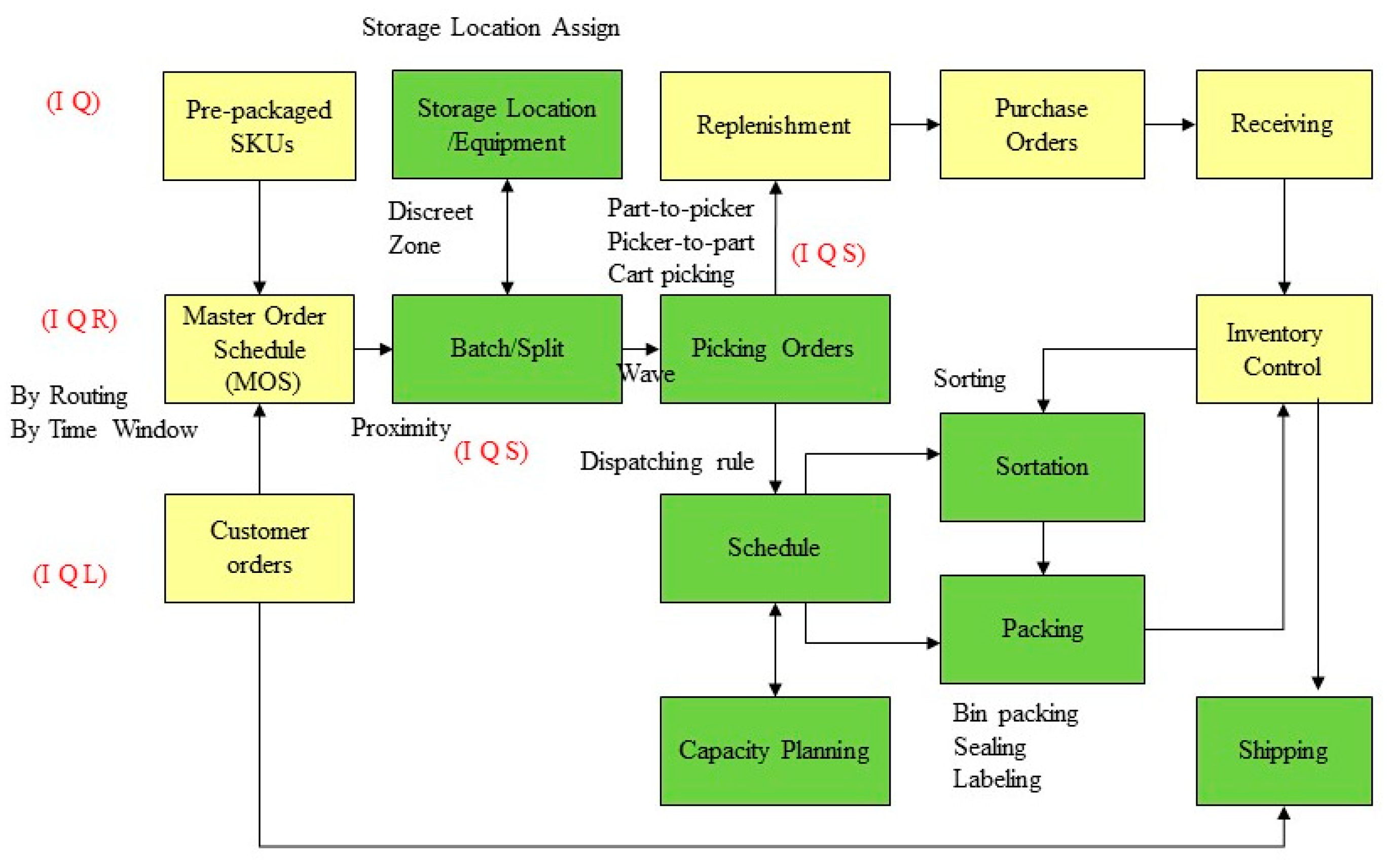
1.3. The Operational Definition of Wave Planning

From WMS perspective, wave picking is one of the most complex functions of the system, because it includes the following planning functions:

• Batching or slitting the customer orders into appropriate picking lists (also called picking orders)
• Locating SKUs in the warehouse
• Creating sequences of picking tasks by considering routing distances
• Release picking tasks to the pickers/equipment to be fulfilled

1.4. The Objective of This Paper

The objective of this research is to develop a mixed integer programming model for wave planning. The model is inspired by a real-world case study of an online bookseller. The model aims to help the bookseller to generate optimal wave picking lists in a given time window. It also can serve as a simulation with the purpose to determine what is the best time window of a wave picking.

2. The Case Study

In Taiwan, 24-h express shipping domestically is one of the promises of an online bookstore. When the promise comes to warehousing, the quality and trustworthiness of the supplier is important. There is a 2-h express warehousing company, located in north of Taiwan, fully supporting the 24-h express shipping for the online bookstore company. The online bookstore company transfers their customer orders, which could be up to around 10,000 orders, to the warehousing company every hour. Based on the customer orders, the warehousing company generates picking orders every 2 h. Currently, picking orders are planned and separated into two categories. One is (type I) picking orders for those customer orders, that only purchase one book. Type I picking orders are also called discrete picking. The other is (type II) picking orders for those customer orders, that purchase two or more books, and type II picking orders are also called batch picking. Carts are devices for those type II picking orders and carts with trays are devices for those type I picking orders. For those type I picking orders, packing processes are as follow placing a box onto a table scale, checking the contents, inserting a pack slip, void filling, and taping. For those type II picking orders, additional sorting orders and packing process are required. Sorting orders is another time-consuming process for warehousing operators. Operators must pick up books from carts and dispatch them into customer-oriented trays as shown in Figure 2. To live up to its reputation of being a 2-h express warehousing company, all the picking and packing processes for around 20,000 customer orders must be done in a 2-h time window.

There are six delivery routes per day in the 2-h express warehousing company. The first group of the delivery routes is called to-door delivery. There is to-door delivery in the morning, to-door delivery in the afternoon, and to-door delivery in the evening. The second group of the delivery routes is called to-store delivery. There is to-store delivery in northern Taiwan, to-store delivery in central Taiwan, and to-store delivery in southern Taiwan. The packed delivery boxes, which are completed every 2 h, will be stacked in a large buffer space and wait for loading to delivery trucks six times per day according to the six delivery routes.

3. Problem Description and Assumptions

3.1. Problem Description

Despite the fact that warehouses have been around for hundreds of years, they continue to evolve because of dramatic changes in customer demands, along with the constant advancements in technology. This is leading to a revolution in warehouse capabilities. According to [16], the global trends of warehousing businesses include (1) higher workforce expectations, (2) continued focus on regulatory compliance, (3) next-generation postponement strategies, (4) increased use of automation and robotics, (5) geographic expansion, (6) increased presence in urban area, (7) compressed order processing times, (8) grater internal and external collaboration, and (9) smart optimization. Basically, to conquer these global trends of warehousing businesses, an enterprise can tackle them by developing new supply chain collaboration strategies, by developing new logistics automation devices, or by developing intelligent mathematic models or algorithms to optimize the warehousing/logistics resources. In this study, we concentrate on tackling the challenge by smart optimization.

This trend of growing online shopping sales has significantly influenced the goods supply chains throughout its international, regional, and last mile segments. Kang [23] pointed trade and logistics businesses have restructured operational and system-wide aspects of their supply chain to accommodate the ever-growing demand for just-in-time (JIT) production, online shopping, and instant shipment/delivery.

To apply JIT concept to order picking process, a number of researches have been tackled jointly in previous studies to provide a comprehensive solution to order picking [6,10,11,12,13,24,25], fulfilling a specified objective function to reduce operational costs [11,12,26,27,28,29], and enhance customer service [10,21,30,31]. We summarized previous studies, that provide integration solutions for order picking processes, as shown in

Table 2. The integrated studies in recent years.

Reference	Integration	Benefit/Goal
Kulak et al. [12]	Order batching, Picker routing	Improve order picking
Hong and Kim [32]
Choy et al. [33]	Order picking, Sequencing
Schubert et al. [34]	Order picking, Vehicle routing	Provide high-quality solutions.
Zhang et al. [4]	Order batching, Delivery	Deliver numerous orders within the shortest time
Won and Olafsson* [6]	Order batching, Order picking	Optimize customer response time.
Chen et al. [10]	Order batching, Sequencing, Routing problem	Minimum total tardiness of customer orders.
Henn [31]	Order batching, Sequencing

.

Recall the case study, stocking packed delivery boxes generated every 2 h is not an efficient way of managing a warehouse. It is not only increasing total travelling paths of all picking operators, but also might waste warehouse buffering space. The idea to improve warehousing efficiency of this case study is to apply JIT concept to order picking process in the 2-h express warehousing company. Try to think about this. Does it make sense to stack packed delivery boxes generated every 2 h (i.e., 2-h based wave planning)? If we can plan order picking waves to as close to as their loading due time as possible, the time with the packed delivery boxes stacking at the buffering space will be reduced, the buffering space for stacking packed delivery boxes will be reduced, and the processing time window from customer orders to picking orders can be expanded, too. With the expanding time windows, more similar order list can then be scheduled into this time frame. The efficiency of the picking operator can be improved.

In this study, we developed a wave planning model to integrate order batching, sequencing, picker routing, packing, and delivery (as green blocks illustrated in Figure 3) for improving warehouse capabilities in terms of reduce buffer spaces and deliver numerous orders within the shortest time.

3.2. Basic Assumption

• The picking area is not zoning.
• The efficiency of pickers is the same.
• The truck loading time is fixed and known.
• Items are cuboid and the length, width and high are known.
• The items, quantity, and correlation of each order are known.
• The picking distance between the storage locations of items are known.
• Candidate containers are cuboid and the cost and the capacity are known.
• The number of pickers, the constrain of picking quantity and the volume capacity of order picker truck are known.
• The distribution center is the kind that can deal with a great amount of orders that are small-volume with large-variety.

4. The Wave Planning Algorithm

In this study, we present a wave planning mathematic model by integrating order picking with packing planning and scheduling by simultaneously consider three major factors: (1) by time window from MOS, (2) random storage SKUs, and (3) picker-to-box.

This model is proposed to the distribution center which focuses on 24-h delivery and the way of picking is by manual picking. Nowadays, the order type of e-commerce is often low-volume and high-mix, and this makes the processes more complicated in the distribution center. How they deal with the e-orders and send the packages to customers within 24 h by the most efficiency way has become the most important goal.

This study extends from Shiau and Liao [17], and takes more factors into consideration (as shown in Figure 4). First, taking the orders as the center, and establish relations with truck loading time, items, batches, containers, and schedule. For example, according to the truck loading time of orders to schedule the batches, and the batch orders to include items and containers for the particular package.

After the distribution center accumulates numerous customers’ orders for 24 h, it should confirm the environment parameters whether should be adjusted. The next step is to consider the relation between picking route, order batching, loading configuration, containers, departure time, and items. The system will calculate the distance from one storage to another. Moreover, it will restrict the picking quantity of each picking order, and compute the shortest picking route and waiting time of containers in the buffer area.

Sets

O = {1,2,...,OR}	set of customer orders
R = {1,2,...,NR}	set of items
BS = {1,2,...,BM}	set of batches
AP = {0,1,...,N}	set of picking points included pickup and deposit (P/D) points
V = {1,2,…,m}	set of candidate containers
$PS=\left\{1\dots ..PE\right\}$	set of pickers
$DR=\left\{1\dots ..ND\right\}$	set of the truck loading time

Relationship matrix

$R{S}_{oi}={\{R{S}_{oi},\dots ,R{S}_{on}\}}^T$

: the relation between orders and items

Parameters

$OR$	: Number of customer orders
$NR$	: Number of items in customer orders
$m$	: Number of candidate containers
$B$	: Batches
$BM$	: Number of batches
$o$	: The customer orders
$i$	: The items customer ordered
j	: The candidate container
$P_{oi}$	: The length of item i in customer order o
$q_{oi}$	: The width of item i in customer order o
$r_{oi}$	: The height of item i in customer order o
$L_j$	: The length of container j
$W_j$	: The width of container j
$H_j$	: The height of container j
$C_j$	: The cost of container j
$t_{ik}$	: The storage distance between item i and item k
$s{d}_b$	: The processing efficiency of batch
$R{S}_{oi}$	: 1 if item i is in order o; 0 otherwise
$PC{P}_b$	: The amount of picking items of each batch b
$PC{B}_p$	: The capacity of the assigned batches by picker p
$EC{P}_b$	: The volume capacity of the order picker cart for batch b
$MAV$	: A very large number
$MAC$	: The maximum cost of packing
$MIC$	: The minimum cost of packing
$MAD$	: The maximum travel distance between items
$MID$	∶ The minimum travel distance between items
MAW	: The maximum waiting time for truck loading
MIW	: The minimum waiting time for truck loading

Input variables

TL	: The limited of total operating time of all pickers
$T_{ir}$	: The truck loading time r of item i
$d{t}_{br}$	: The truck loading time r of batch b

Output variables

$u_{bi}$	: The picking sequence of item i in batch b
$x_{oi}$	: x-axis position of the front-left bottom corner of item i in customer order o be assigned
$y_{oi}$	: y-axis position of the front-left bottom corner of item i in customer order o be assigned
$z_{oi}$	: z-axis position of the front-left bottom corner of item i in customer order o be assigned
$s{p}_b$	∶ The number of total picking points of batch b
$s{t}_{pb}$	: The start time of batch b by picker p
$f{t}_{pb}$	: The finish time of batch b by picker p
$if{t}_{bi}$	: The finish time of item i in batch b
$w{t}_{pb}$	: The waiting time for departure of batch b by picker p
$m{t}_b$	: The operation time of batch b
$ad$	: The total distance of all picking route
$aw$	: The total wait time for truck loading of batches

Decision variables

$S_{oij}$	: 1 if item i is put into box j; 0 otherwise
$n_{oj}$	∶ 1 if box j is used; 0 otherwise
$v_{bi}$	∶ 1 if item i is in batch b; 0 otherwise
$q_{bij}$	∶ 1 if item i of batch b is put into box j; 0 otherwise
$l{x}_{oi}$	∶ 1 if the length of item i is parallel to x-axis of the box; 0 otherwise
$l{y}_{oi}$	∶ 1 if the length of item i is parallel to y-axis of the box; 0 otherwise
$l{z}_{oi}$	∶1 if the length of item i is parallel to z-axis of the box; 0 otherwise
$w{x}_{oi}$	∶ 1 if the width of item i is parallel to x-axis of the box; 0 otherwise
$w{y}_{oi}$	∶ 1 if the width of item i is parallel to y-axis of the box; 0 otherwise
$w{z}_{oi}$	∶ 1 if the width of item i is parallel to z-axis of the box; 0 otherwise
$h{x}_{oi}$	∶ 1 if the height of item i is parallel to x-axis of the box; 0 otherwise
$h{y}_{oi}$	∶ 1 if the height of item i is parallel to y-axis of the box; 0 otherwise
$h{z}_{oi}$	∶ 1 if the height of item i is parallel to z-axis of the box; 0 otherwise
$a_{oik}$	: 1 if item i is on the left side of item k in customer order o; 0 otherwise
$b_{oik}$	: 1 if item i is on the right side of item k in customer order o; 0 otherwise
$c_{oik}$	: 1 if item i is in front of item k in customer order o; 0 otherwise
$d_{oik}$	: 1 if item i is behind item k in customer order o; 0 otherwise
$e_{oik}$	: 1 if item i is under item k in customer order o; 0 otherwise
$f_{oik}$	: 1 if item i is above item k in customer order o; 0 otherwise
$g_{oik}$	: 1 if the picking sequence of item i is before item k in batch B; 0 otherwise
$w_{pb}$	: 1 if batch b is picking by picker p; 0 otherwise

Formulation

• Objective Function

The objective function (1) is to minimize the picking route, the cost of containers and waiting time for truck loading of packaged containers heaping in the buffer area. Since the units of the three factors are different, we have to normalize the three objects.

$$\mathrm{Min}\left(\frac{a d-M I D}{M A D -M I D}+\frac{{{\displaystyle \sum }}_{o=1}^{O R}{{\displaystyle \sum }}_{j=1}^m{C}_j·n_{oj}-M I C}{M A C -M I C}+\frac{a w -M I W}{M A W -M I W}\right)$$

(1)

• Subject to

Constraints (2)–(4) ensure the relation between items and containers. The length, width, and height of each items must be parallel with one axis of the container. For instance, the length of item i is only parallel to x-axis, y-axis, or z-axis of the container (i.e., Equation (2)), where as $l{x}_{oi}$, ${ly}_{oi}$, and ${lz}_{oi}$ are binary variables.

$$l{x}_{oi}+{ly}_{oi}+{lz}_{oi}=1\hspace{1em}\hspace{1em}\hspace{1em}\forall o\in O,i\in R$$

(2)

$${wx}_{oi}+{wy}_{oi}+{wz}_{oi}=1\hspace{1em}\hspace{1em}\hspace{1em}\forall o\in O,i\in R$$

(3)

$$h{x}_{oi}+h{y}_{oi}+h{z}_{oi}=1\hspace{1em}\hspace{1em}\hspace{1em}\forall o\in O,i\in R$$

(4)

In other words, Constraints (5)–(7) ensure what parallel with some axis is one of the lengths, width, or height of item i in order o.

$$l{x}_{oi}+{wx}_{oi}+h{x}_{oi}=1\hspace{1em}\hspace{1em}\hspace{1em}\forall o\in O,i\in R$$

(5)

$$l{y}_{oi}+w{y}_{oi}+h{y}_{oi}=1\hspace{1em}\hspace{1em}\hspace{1em}\forall o\in O,i\in R$$

(6)

$${lz}_{oi}+{wz}_{oi}+h{z}_{oi}=1\hspace{1em}\hspace{1em}\hspace{1em}\forall o\in O,i\in R$$

(7)

Constraints (8)–(13) ensure the relative position how pickers put into the container between item and item in order o. For instance, if item i is on the left side of item k, x-axis position of the front-left bottom corner of item k (i.e., the right-hand side of Equation (8)) must be larger than x-axis position of the front-left bottom corner of item i plus its size of item i is parallel to x-axis of the box (i.e., the left-hand side of Equation (8)).

$$\begin{array}{c}{x}_{oi}+p_{oi}·l{x}_{oi}+q_{oi}·w{x}_{oi}+r_{oi}·h{x}_{oi}\le x_{ok}+\left(1-a_{oik}\right)·MAV\\ \forall o\in O,i\in R,k\in R;i\ne k\end{array}$$

(8)

$$\begin{array}{c}{x}_{oi}+p_{ok}·l{x}_{ok}+q_{ok}·w{x}_{ok}+r_{oi}·h{x}_{ok}\le x_{oi}+\left(1-b_{oik}\right)·MAV\\ \forall o\in O,i\in R,j\in V\end{array}$$

(9)

$$\begin{array}{c}{y}_{oi}+p_{oi}·l{y}_{oi}+q_{oi}·w{y}_{oi}+r_{oi}·h{y}_{oi}\le y_{ok}+\left(1-c_{oik}\right)·MAV\\ \forall o\in O,i\in R,j\in V\end{array}$$

(10)

$$\begin{array}{c}{y}_{ok}+p_{ok}·l{y}_{ok}+q_{ok}·w{y}_{ok}+r_{oi}·h{y}_{ok}\le y_{oi}+\left(1-d_{oik}\right)·MAV\\ \forall o\in O,i\in R,j\in V\end{array}$$

(11)

$$\begin{array}{c}{z}_{oi}+p_{oi}·l{z}_{oi}+q_{oi}·w{z}_{oi}+r_{oi}·h{z}_{oi}\le z_{ok}+\left(1-e_{oik}\right)·MAV\\ \forall o\in O,i\in R,j\in V\end{array}$$

(12)

$$\begin{array}{c}{z}_{ok}+p_{ok}·l{z}_{ok}+q_{ok}·w{z}_{ok}+r_{oi}·h{z}_{ok}\le z_{oi}+\left(1-f_{oik}\right)·MAV\\ \forall o\in O,i\in R,j\in V\end{array}$$

(13)

Constraints (14) ensures the items of the order o are put into the same container. For instance, if in order o, item i (RS_oi = 1) and item k (RS_ok = 1) are put into container j (s_oij = 1 and s_okj = 1), then there exists some correlation between item i and item k.

$$\begin{array}{c}{a}_{oik}+b_{oik}+c_{oik}+d_{oik}+e_{oik}+f_{oik}\ge s_{oij}·R{S}_{oi}+s_{okj}·R{S}_{ok}-1\\ \forall o\in O,i\in R,k\in R,j\in V;i\ne k\end{array}$$

(14)

Constraints (15)–(16) ensure items of order o only put into one container. Only one container j (s_oij) could be equal to one in Equation (15), and in Equation (16) if container j is used (n_oj = 1), item can be put in container j (s_oij >= 0).

$${\displaystyle \sum }_{j=1}^m{s}_{oij}·R{S}_{oi}=1\hspace{1em}\hspace{1em}\hspace{1em}\hspace{1em}\hspace{1em}\hspace{1em}\forall o\in O,i\in R$$

(15)

$${\displaystyle \sum }_{i=1}^{N R}{s}_{oij}·R{S}_{oi}\le MAV·n_{oj}\hspace{1em}\hspace{1em}\hspace{1em}\forall o\in O,j\in V$$

(16)

Constraints (17)–(18) ensure one order can use several containers and the items of different order cannot be put into the same container. In Equation (17), at least one container j must be used for order o. In Equation (18), one container j can only be used in one customer order o.

$${\displaystyle \sum }_{j=1}^m{n}_{oj}\ge 1\hspace{1em}\hspace{1em}\hspace{1em}\forall o\in O$$

(17)

$${\displaystyle \sum }_{o=1}^{OR}{n}_{oj}\le 1\hspace{1em}\hspace{1em}\hspace{1em}\forall j\in V$$

(18)

Constraints (19)–(21) ensure the total size of items putting in the same container is not bigger than the container. For instance, if item i is placed in container j, the size of item i is parallel to x-axis of the box (i.e., the left-hand side of Equation (19)) must be smaller than the size of length of box j (i.e., the right-hand side of Equation (19)).

$$\begin{array}{c}{x}_{oi}+p_{oi}·l{x}_{oi}+q_{oi}·w{x}_{oi}+r_{oi}·h{x}_{oi}\le L_j+\left(1-s_{oij}·R{S}_{oi}\right)·MAV\\ \forall o\in O,i\in R,j\in V\end{array}$$

(19)

$$\begin{array}{c}{y}_{oi}+p_{oi}·l{y}_{oi}+q_{oi}·w{y}_{oi}+r_{oi}·h{y}_{oi}\le W_j+\left(1-s_{oij}·R{S}_{oi}\right)·MAV\\ \forall o\in O,i\in R,j\in V\end{array}$$

(20)

$$\begin{array}{c}{z}_{oi}+p_{oi}·l{z}_{oi}+q_{oi}·w{z}_{oi}+r_{oi}·h{z}_{oi}\le H_j+\left(1-s_{oij}·R{S}_{oi}\right)·MAV\\ \forall o\in O,i\in R,j\in V\end{array}$$

(21)

Constraints (22)–(24) ensure items putting in the same container must be in the same batch. In Equation (22) only one batch b is used for a container j (i.e., only one q_bij could be equal to 1). In Equation (23) if item i and item k are in the same container j (s_oij = 1 and s_okj = 1), they must be in the same batch b (q_bij = 1 and q_bkj = 1). Equation (24) determines those container j for item i (q_bij = 1) if item i is assigned to batch b (v_bi = 1).

$${\displaystyle \sum }_{j=1}^m\left({\displaystyle \sum }_{b=1}^{B M}{q}_{bij}\right)·s_{oij}·R{S}_{oi}=1\hspace{1em}\hspace{1em}\hspace{1em}\forall o\in O,i\in R$$

(22)

$$q_{bij}·s_{oij}·R{S}_{oi}-q_{bkj}·s_{okj}·R{S}_{ok}=0\hspace{1em}\forall b\in BS,o\in O,i\in R,j\in V;ik$$

(23)

$${\displaystyle \sum }_{j=1}^m{q}_{bij}=v_{bi}\hspace{1em}\hspace{1em}\hspace{1em}\forall b\in BS,i\in R$$

(24)

Constraints (25) ensures every picker starts with P/D point.

$$v_{b0}=1\hspace{1em}\hspace{1em}\hspace{1em}\forall b\in BS$$

(25)

Constraints (26)–(27) ensure each order picker cart (ECP_b) does not overload and the picking quantities do not exceed the capability of each picking operator (PCP_b).

$${\displaystyle \sum }_{i=1}^{N R}{\displaystyle \sum }_{j=1}^m{L}_j·W_j·H_j·q_{bij}·s_{oij}·R{S}_{oi}\le EC{P}_b\hspace{1em}\forall b\in BS,o\in O$$

(26)

$${\displaystyle \sum }_{i=1}^{N R}{v}_{bi}\le PC{P}_b\hspace{1em}\hspace{1em}\hspace{1em}\hspace{1em}\hspace{1em}\hspace{1em}\forall b\in BS$$

(27)

Constraints (28)–(30) calculate the total distant (ad) and ensure pickers will not walk to the repeated route. For instance, if item 1 is picked before item 2, and item 2 is picked before item 3, then it is not possible for item 3 to be picked before item 1.

$${\displaystyle \sum }_{b=1}^{B M}{\displaystyle \sum }_{j=1}^m{\displaystyle \sum }_{i=1}^{N R}{\displaystyle \sum }_{k=0}^{N R}{t}_{ik}·g_{bik}·v_{bi}·v_{bk}=ad\hspace{1em}\hspace{1em}i\ne k$$

(28)

$${\displaystyle \sum }_{k=1}^{N R}{g}_{b0k}·v_{b0}·v_{bk}=1\hspace{1em}\hspace{1em}\hspace{1em}\forall b\in BS$$

(29)

$${\displaystyle \sum }_{b=1}^{B M}{\displaystyle \sum }_{i=0}^{N R}{g}_{bik}·v_{bi}·v_{bk}=1\hspace{1em}\hspace{1em}\hspace{1em}\forall k\in AP;i\ne k$$

(30)

Constraints (31)–(33) ensure pickers will walk from one picking point to another and finally back to P/D point. In Equation (31) each batch b, only one item i can be picked after P/D point (i.e., only one $g_{bi0}$ could be equal to 1). In Equation (32), for each batch b, only one item k can be picked after item i (i.e., only one $g_{bi0}$ could be equal to 1). In Equation (33), the number of total picking points of batch b is calculated.

$${\displaystyle \sum }_{i=1}^{N R}{g}_{bi0}·v_{bi}·v_{b0}=1\hspace{1em}\hspace{1em}\hspace{1em}\forall b\in BS$$

(31)

$${\displaystyle \sum }_{b=1}^{B M}{\displaystyle \sum }_{k=0}^{N R}{g}_{bik}·v_{bi}·v_{bk}=1\hspace{1em}\hspace{1em}\hspace{1em}\forall i\in AP;i\ne k$$

(32)

$${\displaystyle \sum }_{i=1}^{N R}{v}_{bi}=s{p}_b\hspace{1em}\hspace{1em}\hspace{1em}\hspace{1em}\hspace{1em}\forall b\in B$$

(33)

Constraints (34) determines picking sequence of each item i (u_bi) and item k (u_bk).

$$\begin{array}{c}{u}_{bi}-u_{bk}+\left(s{p}_b+1\right)·g_{bik}\le s{p}_b+\left(1-v_{bi}·v_{bk}\right)·MAV\\ \forall b\in BS,i\in AP,k\in R;i\ne k\end{array}$$

(34)

If items in the batches, the picking sequence of items (u_bi) should be more than or equal to zero by Constraints (35)–(36).

$$u_{bi}\le s{p}_b+\left(1-v_{bi}\right)·MAV\hspace{1em}\hspace{1em}\forall b\in BS,i\in AP$$

(35)

$$u_{bi}\ge 0-\left(1-v_{bi}\right)·MAV\hspace{1em}\hspace{1em}\hspace{1em}\forall b\in BS,i\in AP$$

(36)

Constraints (37)–(38) ensure the items placing in the lower position of containers will be picked first. If item i is placed in lower layer to item k (i.e., $e_{oik}$ = 1 and $f_{oik}=0$), then Equations (37) and (38) are held.

$$\begin{array}{c}{e}_{oik}\left(u_{bi}-u_{bk}\right)\le 0+\left(1-v_{bi}·v_{bk}\right)·MAV\\ \forall b\in BS,o\in O,i\in R,k\in R;i\ne k\end{array}$$

(37)

$$\begin{array}{c}{f}_{oik}\left(u_{bi}-u_{bk}\right)\ge 0-\left(1-v_{bi}·v_{bk}\right)·MAV\\ \forall b\in BS,o\in O,i\in R,k\in R;i\ne k\end{array}$$

(38)

Constraints (39)–(40) determine how to assign the batch to pickers. In Equation (39), a picker p can be only assigned to one batch b. Equation (40) calculates the capacity of the assigned batches (PCB_p) by picker p.

$${\displaystyle \sum }_{p=1}^{P E}{W}_{pb}=1\hspace{1em}\hspace{1em}\hspace{1em}\forall b\in BS$$

(39)

$${\displaystyle \sum }_{b=1}^{B M}{W}_{pb}=PC{B}_p\hspace{1em}\hspace{1em}\forall p\in PS$$

(40)

Constraint (41) calculates the operation time of batch (mt_b).

$${\displaystyle \sum }_{i=1}^{N R}{\displaystyle \sum }_{k=1}^{N R}{t}_{ik}·g_{bik·}{v}_{bi}·v_{bk}·s{d}_b=m{t}_b\hspace{1em}\hspace{1em}i\ne k$$

(41)

Constraint (42) limits the total operation time.

$${\displaystyle \sum }_{b=1}^{B M}m{t}_b·W_{pb}\le TL\hspace{1em}\hspace{1em}\hspace{1em}\hspace{1em}\hspace{1em}\hspace{1em}\forall b\in BS$$

(42)

Constraint (43) calculates the start time of batch (st_pb).

$$s{t}_{pb}+m{t}_b\ast W_{pb}\le {ft}_{pb}\hspace{1em}\hspace{1em}\forall p\in PS;\forall b\in BS$$

(43)

Constraint (44) ensures the sequence of batches (i.e., finish time of batch b must less than start time of batch k).

$${ft}_{pb}\le s{t}_{pk}\hspace{1em}b\ne k;\forall p\in PS;\forall b\in BS;\forall k\in BS$$

(44)

Constraint (45) calculates the waiting time for truck loading (wt_pb) of batches.

$${ft}_{pb}+w{t}_{pb}=d{t}_{br}\hspace{1em}\forall p\in PS;\forall b\in BS;\forall r\in DR$$

(45)

Constraint (46) is the finish time of batch b to be equal to the finish time of items in batch b. In Constraint (47), all finish time of items in batch b (ift_bi) must be earlier than the given due time (T_ir).

$$i{ft}_{bi}={ft}_{pb}·v_{bi}\hspace{1em}\hspace{1em}\forall p\in PS;\forall b\in BS;\forall i\in AP$$

(46)

$$i{ft}_{bi}\le T_{ir}\hspace{1em}\hspace{1em}\hspace{1em}\hspace{1em}\forall b\in BS;\forall i\in AP;\forall r\in DR$$

(47)

Constraint (48) calculates the total waiting time of batches (aw).

$${\displaystyle \sum }_{p=1}^{PE}{\displaystyle \sum }_{b=1}^{BM}w{t}_{pb}=aw$$

(48)

$$x_{oi},y_{oi},z_{oi},{ft}_{pb},i{ft}_{bi},w{t}_{pb}\ge 0$$

(49)

Constraints (50)–(51) declare the 0/1 variables and nonnegative variables in this model.

$$l{x}_{oi},l{y}_{oi},l{z}_{oi},w{x}_{oi},w{y}_{oi},w{z}_{oi},h{x}_{oi},h{y}_{oi},h{z}_{oi}=0,1$$

(50)

$$a_{oik},b_{oik},c_{oik},d_{oik},e_{oik},f_{oik},g_{bik},s_{oij},n_{oj},q_{bij},v_{bi},W_{pb}=0,1$$

(51)

5. The Example Sets

This study takes the distribution center of the e-retailer of a bookstore for example. We suppose the working time will be from 6:00 a.m. to 10:00 p.m. and they will fulfill customers’ orders within 24 h. If customers place the orders before 12:00 p.m., they will receive the items on the following day before 12:00 p.m. However, if they place the orders after 12:00 p.m., they will receive the items until the day after tomorrow before 12:00 p.m.

The e-commerce will send a batch of orders to the distribution center every two hours and the distribution center will start to deal the orders rapidly before the next batch arrives. The problem with this is that it will mean that many packages will be waiting for delivery in the buffer area. Another problem is that the pickers may travel to the same locations every two hours.

By wave planning, the distribution center can accumulate the batches of orders which the e-commerce sends every two hours. After 24 h, the distribution center will transfer the customer orders to picking orders at 6:00 a.m. and 12:00 p.m. according to the truck loading time and items of the orders. Before pickers start to pick, they need to set up the environment parameters. Then, use the optimization modeling software to solve the problem.

First, the setup of WMS including the storage location of items, the type of containers, the capacity of pickers, and the volume capacity of order picker trucks. There are 32 items, numbered from 1 to 32, and the storage locations are transferred as a distance matrix. Containers have three kinds of sizes showed in

Table 3. The sizes and price of three kinds of containers.

Container Number (j)	Container Graph	Container Size (cm)			Price (C)
		Length $\left({\mathit{L}}_{\mathit{j}}\right)$	Width $\left({\mathit{W}}_{\mathit{j}}\right)$	Height $\left({\mathit{H}}_{\mathit{j}}\right)$
Size 1 (j = 1~7)		23	14	13	55
Size 2 (j = 8~20)		23	18	19	70
Size 3 (j = 21~27)		39.5	27.5	23	100

. To assign the jobs to pickers equally, the capacity of pickers is the same (let us say 4 units/each) and the volume capacity of order picker trucks are also the same (let us say 149,903 cm³/unit). According to the difference delivery place, there are five truck loading times, which are (1) 9 a.m. for south shop delivery, (2) 3 p.m. for central shop delivery, (3) 10 p.m. for north shop delivery, (4) 12 p.m. for to-door delivery, and (5) 5 p.m. for another to-door delivery.

After inputting the environment parameters, it can start to check the information of customer orders including item number, quantities, and item size (see

Table 4. The customer orders.

Place Order Time	Customer Order $\left(\mathit{o}\right)$	Item Number $\left(\mathit{i}\right)$	Quantity	Item Size (cm)			Truck Loading Time (r) (The Next Day)
				Length $\left({\mathit{p}}_{\mathit{o}\mathit{i}}\right)$	Width $\left({\mathit{q}}_{\mathit{o}\mathit{i}}\right)$	Height $\left({\mathit{r}}_{\mathit{o}\mathit{i}}\right)$
12–14	1	3	1	13	5	6	3 p.m.
		8	1	20	10	10	3 p.m.
14–16	2	9	1	15	13	10	9 a.m.
		10	1	17	12	13	9 a.m.
	3	11	1	14	13	5	9 a.m.
		17	1	5	5	10	9 a.m.
	4	12	1	7	14	7	9 a.m.
		13	1	16	4	5	9 a.m.
16–18	5	1	1	5	3	6	9 a.m.
		2	1	16	19	7	9 a.m.
	6	4	1	8	4	7	3 p.m.
		14	1	13	5	5	3 p.m.
	7	6	1	14	8	5	5 p.m.
		7	1	8	4	4	5 p.m.
	8	15	1	5	5	10	5 p.m.
		23	1	15	10	6	5 p.m.
	9	5	1	13	5	6	12 p.m.
		18	1	20	10	10	12 p.m.
18–20	10	19	1	15	13	10	12 p.m.
		20	1	17	12	13	12 p.m.
20–22	11	21	1	14	13	5	12 p.m.
		24	1	5	5	10	12 p.m.
22–24	12	16	1	7	14	7	12 p.m.
		22	1	16	4	5	12 p.m.
4–6	13	25	1	13	5	6	10 p.m.
		26	1	20	10	10	10 p.m.
6–8	14	31	1	15	13	10	10 p.m.
		32	1	17	12	13	10 p.m.
8–10	15	27	1	14	13	5	10 p.m.
		29	1	5	5	10	10 p.m.
10–12	16	28	1	7	14	7	10 p.m.
		30	1	16	4	5	10 p.m.

). Then the system would generate the relation between customer orders and items $R{S}_{oi}$ (see

Table 5. The relation matrix of customer orders and items ($R{S}_{oi}$).

	Order (o)	1	2	3	4	5	6	7	8	9	10	11	12	13	14	15	16
Item (i)
1		0	0	0	0	1	0	0	0	0	0	0	0	0	0	0	0
2		0	0	0	0	1	0	0	0	0	0	0	0	0	0	0	0
3		1	0	0	0	0	0	0	0	0	0	0	0	0	0	0	0
4		0	0	0	0	0	1	0	0	0	0	0	0	0	0	0	0
5		0	0	0	0	0	0	0	0	1	0	0	0	0	0	0	0
6		0	0	0	0	0	0	1	0	0	0	0	0	0	0	0	0
7		0	0	0	0	0	0	1	0	0	0	0	0	0	0	0	0
8		1	0	0	0	0	0	0	0	0	0	0	0	0	0	0	0
9		0	1	0	0	0	0	0	0	0	0	0	0	0	0	0	0
10		0	1	0	0	0	0	0	0	0	0	0	0	0	0	0	0
11		0	0	1	0	0	0	0	0	0	0	0	0	0	0	0	0
12		0	0	0	1	0	0	0	0	0	0	0	0	0	0	0	0
13		0	0	0	1	0	0	0	0	0	0	0	0	0	0	0	0
14		0	0	0	0	0	1	0	0	0	0	0	0	0	0	0	0
15		0	0	0	0	0	0	0	1	0	0	0	0	0	0	0	0
16		0	0	0	0	0	0	0	0	0	0	0	1	0	0	0	0
17		0	0	1	0	0	0	0	0	0	0	0	0	0	0	0	0
18		0	0	0	0	0	0	0	0	1	0	0	0	0	0	0	0
19		0	0	0	0	0	0	0	0	0	1	0	0	0	0	0	0
20		0	0	0	0	0	0	0	0	0	1	0	0	0	0	0	0
21		0	0	0	0	0	0	0	0	0	0	1	0	0	0	0	0
22		0	0	0	0	0	0	0	0	0	0	0	1	0	0	0	0
23		0	0	0	0	0	0	0	1	0	0	0	0	0	0	0	0
24		0	0	0	0	0	0	0	0	0	0	1	0	0	0	0	0
25		0	0	0	0	0	0	0	0	0	0	0	0	1	0	0	0
26		0	0	0	0	0	0	0	0	0	0	0	0	1	0	0	0
27		0	0	0	0	0	0	0	0	0	0	0	0	0	0	1	0
28		0	0	0	0	0	0	0	0	0	0	0	0	0	0	0	1
29		0	0	0	0	0	0	0	0	0	0	0	0	0	0	1	0
30		0	0	0	0	0	0	0	0	0	0	0	0	0	0	0	1
31		0	0	0	0	0	0	0	0	0	0	0	0	0	1	0	0
32		0	0	0	0	0	0	0	0	0	0	0	0	0	1	0	0

) and the item number i is the picking point i. The start and finish place of pickers are P/D point, and the number of picking points is showed in

Table 6. The item numbers and picking point numbers.

Item Number (i)	-	1	2	3	4	5	6	7	8	9	10
Storage location	P/D	F9	G6	D14	I13	K7	J4	I9	E2	D7	E2
Picking Point (i)	33	1	2	3	4	5	6	7	8	9	10
Item number (i)	11	12	13	14	15	16	17	18	19	20	21
Storage location	F1	F5	G12	H8	I3	J6	F14	J11	K13	K14	H14
Picking Point (i)	11	12	13	14	15	16	17	18	19	20	21
Item number (i)	22	23	24	25	26	27	28	29	30	31	32
Storage location	J15	K10	H3	J12	B14	B12	E12	D11	B10	C13	I11
Picking Point (i)	22	23	24	25	26	27	28	29	30	31	32

. Compared to the five truck loading schedules, an associated truck loading time is assigned to each item which ensures the items will be picked before the truck loading time.

Table 7. The distance between picking point.

	1	2	3	4	5	6	7	8	9	10	11	12	13	14	15	16	17	18	19	20	21	22	23	24	25	26	27	28	29	30	31	32	33
1	0	3	12	13	22	19	17	18	19	15	8	3	3	18	14	21	5	18	16	15	12	14	19	15	17	15	17	14	15	19	16	15	7
2	3	0	15	16	19	16	18	15	16	12	5	1	6	17	11	18	8	21	19	18	15	17	22	12	20	18	20	17	18	22	19	18	10
3	12	15	0	11	20	23	15	18	7	11	18	16	9	12	22	21	7	16	14	13	10	12	17	21	15	7	9	2	3	11	8	13	5
4	13	16	11	0	15	18	4	25	18	22	17	17	10	5	11	16	8	11	9	8	1	7	12	10	10	14	16	13	14	18	15	2	6
5	22	19	20	15	0	3	19	22	23	19	14	18	19	20	12	1	17	4	5	7	14	8	3	13	5	23	25	22	23	27	24	17	15
6	19	16	23	18	3	0	16	19	20	16	11	15	22	15	9	2	20	7	9	10	17	11	6	10	8	26	28	25	24	26	27	18	18
7	17	18	15	4	19	16	0	21	22	18	13	17	14	1	7	18	12	15	13	12	5	11	16	6	14	18	20	17	18	22	19	2	10
8	18	15	18	25	22	19	21	0	13	9	10	14	22	20	14	21	21	30	28	27	25	26	24	26	27	12	10	17	16	8	11	22	19
9	19	16	7	18	23	20	22	13	0	5	11	15	16	23	15	22	14	23	21	20	17	19	24	16	22	14	16	5	4	18	15	20	12
10	15	12	11	22	19	16	18	9	5	0	7	11	18	17	11	18	18	23	25	24	22	24	21	11	24	19	17	10	9	15	20	19	16
11	8	5	18	17	14	11	13	10	11	7	0	4	11	12	6	13	13	18	20	21	18	22	17	7	19	21	19	16	15	17	20	15	15
12	3	1	16	17	18	15	17	14	15	11	4	0	7	16	10	17	9	22	20	19	16	18	21	11	21	19	21	18	19	21	20	19	11
13	3	6	9	10	19	22	14	22	16	18	11	7	0	15	21	20	2	15	13	12	9	11	16	18	14	12	14	11	12	16	13	12	4
14	18	17	16	5	20	15	1	20	23	17	12	16	15	0	6	17	13	16	14	13	6	12	17	5	15	19	21	18	19	23	20	3	11
15	14	11	22	11	12	9	7	14	15	11	6	10	21	6	0	11	19	16	20	19	12	18	15	1	17	25	23	20	19	21	24	9	17
16	21	18	21	16	1	2	18	21	22	18	13	17	20	17	11	0	18	5	7	8	15	9	4	12	6	24	26	23	24	28	25	18	16
17	5	8	7	8	17	20	12	21	14	18	13	9	2	13	19	18	0	13	11	10	7	9	14	18	12	10	12	9	10	14	11	10	2
18	18	21	16	11	4	7	15	30	23	23	18	22	15	16	16	5	13	0	2	3	10	4	1	17	1	19	21	18	19	23	20	13	11
19	16	19	14	9	6	9	13	28	21	25	20	20	13	14	20	7	11	2	0	1	8	2	3	19	1	17	19	16	17	21	18	11	9
20	15	18	13	8	7	10	12	27	20	24	21	19	12	13	19	8	10	3	1	0	7	1	4	18	2	16	18	15	16	20	17	10	8
21	12	15	10	1	14	17	5	25	17	22	18	16	9	6	12	15	7	10	8	7	0	6	11	11	9	13	15	12	13	17	14	3	5
22	14	17	12	7	8	11	11	26	19	24	22	18	11	12	18	9	9	4	2	1	6	0	5	17	3	15	17	14	15	19	18	9	7
23	19	22	17	12	3	6	16	24	24	21	17	21	16	17	15	4	14	1	3	4	11	5	0	16	2	20	22	19	20	24	23	14	12
24	15	12	21	10	13	10	6	14	16	11	7	11	18	5	1	12	18	17	19	18	11	17	16	0	18	24	24	23	24	22	25	18	16
25	17	20	15	10	5	8	14	27	22	24	19	21	14	15	17	6	12	1	1	2	9	3	2	18	0	18	20	17	18	22	19	12	10
26	15	18	7	14	23	26	18	12	14	19	21	19	12	19	25	24	10	19	17	16	13	15	20	24	18	0	2	9	10	4	1	16	8
27	17	20	9	16	25	28	20	10	16	17	19	21	14	21	23	26	12	21	19	18	15	17	22	24	20	2	0	11	12	2	1	18	10
28	14	17	2	13	22	25	17	17	5	10	16	18	11	18	20	23	9	18	16	15	12	14	19	23	17	9	11	0	1	13	10	15	7
29	15	18	3	14	23	24	18	16	4	9	15	19	12	19	19	24	10	19	17	16	13	15	20	24	18	10	12	1	0	14	11	16	8
30	19	22	11	18	27	26	22	8	18	15	17	21	16	23	21	28	14	23	21	20	17	19	24	22	22	4	2	13	14	0	3	20	12
31	16	19	8	15	24	27	19	11	15	20	20	20	13	20	24	25	11	20	18	17	14	18	23	25	19	1	1	10	11	3	0	17	9
32	15	18	13	2	17	18	2	22	20	19	15	19	12	3	9	18	10	13	11	10	3	9	14	8	12	16	18	15	16	20	17	0	8
33	7	10	5	6	15	18	10	19	12	16	15	11	4	11	17	16	2	11	9	8	5	7	12	16	10	8	10	7	8	12	9	8	0

is the distance between picking point.

Table 8. The performance of picking before using the module.

Placing Order Time	Processing Time	Batch (b)	Customer Order (o)	Operation Time	Waiting Time $\left(\mathit{w}{\mathit{t}}_{\mathit{p}\mathit{b}}\right)$	Truck Loading Time (r)
12–14	14–16	1	1	21	1380 min.	3 p.m. of the next day
14–16	16–18	2	2	20	900 min.	9 a.m. of the next day
			3		900 min.	9 a.m. of the next day
		3	4	11	900 min.	9 a.m. of the next day
16–18	18–20	4	5	19	780 min.	9 a.m. of the next day
			6		1140 min.	3 p.m. of the next day
		5	7	22	1200 min.	5 p.m. of the next day
			8		1200 min.	5 p.m. of the next day
		6	9	15	960 min.	12 p.m. of the next day
18–20	20–22	7	10	9	840 min.	12 p.m. of the next day
20–22	The next day 6–8	8	11	22	240 min.	12 p.m. of the next day
22–24			12		240 min.	12 p.m. of the next day
4–6 of the next day		9	13	18	840 min.	10 p.m. of the next day
6–8 of the next day	The next day 8–10	10	14	17	720 min.	10 p.m. of the next day
8–10 of the next day	The next day 10–12	11	15	15	600 min.	10 p.m. of the next day
10–12 of the next day	The next day 12–14	12	16	18	480 min.	10 p.m. of the next day

is the performance of picking before using the model. The calculation of operation time is the distance multiplied by the processing efficiency and the waiting time starts from the final of that processing time window. For example, if the processing time is 2–4 p.m., trucking loading time is 3 p.m. of the next day. The waiting time will start from 4 p.m. to 3 p.m. of the next day. The total waiting time is 13,320 min and the total operation time is 207 min.

6. The Computational Results

This study accumulates the customer orders for 24 h from 12:00 p.m. to 12:00 p.m. of the next day. If the customer orders were placed within the period of 12:00 p.m. to 6 a.m. of the next day, and to be delivered to the south and home before 12:00 p.m., the wave planning module would generate the picking schedule at 6:00 a.m. on the next day. If orders were placed within the period of 12:00 p.m. to 12:00 p.m. of the next day and to be delivered to the north shop, central shop, and home before 17:00 p.m., the wave planning module would generate the picking schedule at 12:00 p.m. of the next day.

There are 16 orders assign to two pickers and dividing into eight batches (

Table 9. The improvement results.

Batch (b)/Picker (p)	Placing Order Time	Customer Order (o)	Start Time $\left(\mathit{s}{\mathit{t}}_{\mathit{p}\mathit{b}}\right)$	Operation Time (min.) $(\mathit{m}{\mathit{t}}_{\mathit{b}})$	Finish Time $\left(\mathit{f}{\mathit{t}}_{\mathit{p}\mathit{b}}\right)$	Waiting Time $\left(\mathit{w}{\mathit{t}}_{\mathit{p}\mathit{b}}\right)$	Truck Loading Time (r)
1/1	14–16	2	8:23 a.m.	26	8:49 a.m.	11 min.	12:00 p.m.
	14–16	3				11 min.	12:00 p.m.
2/1	14–16	4	8:49 a.m.	11	9:00 a.m.	0	12:00 p.m.
	16–18	5					12:00 p.m.
3/1	16–18	9	11:22 a.m.	16	11:38 a.m.	22 min.	12:00 p.m.
	22–24	12				22 min.	12:00 p.m.
4/2	18–20	10	11:38 a.m.	22	12:00 p.m.	0	12:00 p.m.
	20–22	11					12:00 p.m.
5/1	12–14	1	2:33 p.m.	27	3:00 p.m.	0	5:00 p.m.
	16–18	6					5:00 p.m.
6/2	16–18	7	4:34 p.m.	22	5:00 p.m.	0	5:00 p.m.
	16–18	8					5:00 p.m.
7/2	8–10	15	9:11 p.m.	17	9:28 p.m.	32 min.	10:00 p.m.
	10–12	16				32 min.	10:00 p.m.
8/2	4–6	13	9:28 p.m.	32	10:00 p.m.	0	10:00 p.m.
	6–8	14					10:00 p.m.

). In this case, the result is a feasible solution (Figure 5). The planned waves are showed in Figure 6. The total waiting time is 65 min and operation time is 173 min. The total picking route is 346 m and the total cost of container price is 1030 dollars (

Table 10. The packaged container of customer orders.

Batch (b)	Customer Orders (o)	Container (j)	Container size	Container Price ( ${\mathit{C}}_{\mathit{j}}$)
1	2	14	2	70
	3	2	1	55
2	4	13	2	70
	5	8	2	70
3	9	15	2	70
	12	11	2	70
4	10	10	2	70
	11	7	1	55
5	1	9	2	70
	6	5	1	55
6	7	6	1	55
	8	20	2	70
7	15	3	1	55
	16	1	1	55
8	13	16	2	70
	14	19	2	70

).

The system will compute the most suitable container and the sequence of putting the items into the containers is done according to the picking sequence (

Table 11. The picking sequence of items in batch b.

	Batch (b)	1	2	3	4	5	6	7	8
$\mathrm{Picking}$ $\mathrm{Sequence}$ $\mathrm{of} \mathrm{Items}$ $({\mathit{u}}_{\mathit{b}\mathit{i}})$
1		0	2	0	0	0	0	0	0
2		0	4	0	0	0	0	0	0
3		0	0	0	0	1	0	0	0
4		0	0	0	0	4	0	0	0
5		0	0	4	0	0	0	0	0
6		0	0	0	0	0	3	0	0
7		0	0	0	0	0	1	0	0
8		0	0	0	0	2	0	0	0
9		2	0	0	0	0	0	0	0
10		3	0	0	0	0	0	0	0
11		1	0	0	0	0	0	0	0
12		0	3	0	0	0	0	0	0
13		0	1	0	0	0	0	0	0
14		0	0	0	0	3	0	0	0
15		0	0	0	0	0	2	0	0
16		0	0	3	0	0	0	0	0
17		4	0	0	0	0	0	0	0
18		0	0	2	0	0	0	0	0
19		0	0	0	2	0	0	0	0
20		0	0	0	1	0	0	0	0
21		0	0	0	3	0	0	0	0
22		0	0	1	0	0	0	0	0
23		0	0	0	0	0	4	0	0
24		0	0	0	4	0	0	0	0
25		0	0	0	0	0	0	0	2
26		0	0	0	0	0	0	0	1
27		0	0	0	0	0	0	4	0
28		0	0	0	0	0	0	1	0
29		0	0	0	0	0	0	2	0
30		0	0	0	0	0	0	3	0
31		0	0	0	0	0	0	0	4
32		0	0	0	0	0	0	0	3

). The loading configuration is also generated.

Before Lingo 13.0 was used to find the model solution, the limit was increased to 50,000 through the general memory limit under options to facilitate a smooth solution-finding process.

(1)

Model output: The model solution was found using the Lingo 13.0 optimization program. Figure 5 presents the Lingo solution-finding result screen.

(2)

Numbers of decision variables and constraint equations:

Number of decision variables: 32,098;

Number of constraint equations: 18,722;

Model efficiency:

Number of solution-finding cycles: 3,257,849;

Number of solution-finding steps: 3837;

Time used to solve the model: 5 h 57 min and 42 s.

After calculating the performance, waiting time of the original picking planning is 13,320 min, operation time of the original picking planning is 207 min, and the total distance traveled for the original picking planning is 414 m. The calculated waiting time of the wave planning is 130 min, operation time of the wave planning is 173 min, and the total distance traveled for the wave planning logic is 346 m.

Figure 6 illustrates the Gantt chart of the eight batches for the two pickers. For example, the picking route of batch one is showed in Figure 7. Picker 1 will start to pick from P/D point at 8:23 a.m., and the picking sequence is 11→9→10→17. After picking the four items, Picker 1 would go back to P/D point at 8:49 a.m. The load configuration of order 2 and order 3 are showed in Figure 8. The container size of order 2 is size two and order 3 is size one.

After fulfilling the batch one, Picker 1 will start to deal batch two continually. Picker 1 will start to pick from P/D point at 8:49 am, and the picking sequence is 13→1→12→2. After picking the four items, Picker 1 would back to P/D point at 9:00 am. The container size of order 4 and 5 is size two.

Picker 1 will start to pick from P/D point at 11:22 am, and the picking sequence is 22→18→16→5. After picking the four items, Picker 1 would back to P/D point at 11:38 am. The container size of order 9 and 12 is size two.

At 2:33 pm, the Picker 1 will start to deal with batch five. Picker 1 will start to pick from P/D point at 2:33 pm, and the picking sequence is 3→8→14→4. After picking the four items, Picker 1 would back to P/D point at 3:00 pm. The container size of order 1 is size two and order 6 is size one.

Comparing the waiting times, operation times, total travelling distances between original picking planning, and proposed wave planning, the results shown that the wave planning model can reduce the waiting time for truck loading of packages significantly, and also can reduce the time packages heaping in buffer area. The operation time and total distance of picking route also have better results when tested with wave planning.

The characteristics of the SKUs being handled, total number of transactions, total number of orders, picks per order, quantity per pick, total number of SKUs, value-added processing activities such as kitting or private labeling, and handling of piece pick, case pick, or full-pallet loads are all factors that affect the method for order picking. Comparing with previous studies as shown in Table 2, our model demonstrated a successful integration of batching and splitting customer orders, sequencing picking orders, planning picker routes, scheduling picking waves, assigning packing configurations, and eliminating packing operations. Moreover, it also can increase capacity utilization rate and reduce the packaging cost.

7. Conclusions

Order picking policy is a case-oriented design and planning task. In this paper, we reviewed an order picking problem from forms and workflow of a WMS perspectives. By using them to observe an order picking problem of a 24-h express shipping online bookstore, the considering parameters of wave planning for designing the optimization programming model were identified.

To the best of our knowledge, there was no wave order picking planning algorithm been revealed so far. The wave planning model we developed was a mixed integer nonlinear programming model. It takes multiple customer orders, SKUs’ sizes, volumes of mailing boxes, locations of SKUs, and planned delivering truck loading times as input parameters, then calculates the configuration of containers (i.e., bin packing problem), the groups of picking SKUs (i.e., order batch problem), and the groups of pickers (i.e., batch assignment problem), and, finally, outputs a set of order picking lists with their associated schedules.

The past studies showed that picking orders in a short time window is a better picking policy in the random storage warehouse [5]. However, having our proposed model, distribution centers can adjust the frequency of order batching. In other words, the distribution center can accumulate orders for a longer time window which may collect more similar SKUs. The combined picking of several orders can bring about a reduction of approximately 60% in walking time [2]. Moreover, this can avoid order pickers to travel to the same storage locations in the short time. To sum up, the object of the model is that distribution centers can not only achieve the goal of fast delivering but also increase the capacity utilization rate which can make distributions fulfill more orders within the same time period and can completed orders before departure time.

The proposed model is a nonlinear mixed integer programming model. The limitation to this kind of model is that the derivation of an optimal solution is not always guaranteed. Therefore, we could only use an example to prove the capability of the conceptual design of such an order picking system. The calculating time of the example is around 6 h, which also makes the practical use of this model limited. This brings the need of developing a heuristic algorithm for finding the near optimal solution of our model in a relative short computing time as our future work. Our current model could be used as a benchmark reference model for comparing solution results while developing such heuristic algorithms.

References

1. Chabot, T.; Lahyani, R.; Coelho, L.C.; Renaud, J. Order picking problems under weight, fragility and category constraints. Int. J. Prod. Res. 2016, 55, 6361–6379. [Google Scholar] [CrossRef]
2. Brynzér, H.; Johansson, M. Design and performance of kitting and order picking systems. Int. J. Prod. Econ. 1995, 41, 115–125. [Google Scholar] [CrossRef]
3. Sharp, G.P.; Il-Choe, K.; Yoon, C.S.; Graves, R.J.; Wilhelm, M.R.; McGinnis, L.F.; Ward, R.E. Small Parts Order Picking: Analysis Framework and Selected Results. In Material Handling’90; Springer: Berlin/Heidelberg, Germany, 1991; pp. 317–341. [Google Scholar]
4. Zhang, J.; Wang, X.; Huang, K. Integrated on-line scheduling of order batching and delivery under B2C e-commerce. Comput. Ind. Eng. 2016, 94, 280–289. [Google Scholar] [CrossRef]
5. De Koster, R.; Le-Duc, T.; Roodbergen, K.J. Design and control of warehouse order picking: A literature review. Eur. J. Oper. Res. 2007, 182, 481–501. [Google Scholar] [CrossRef]
6. Won, J. Joint order batching and order picking in warehouse operations. Int. J. Prod. Res. 2005, 43, 1427–1442. [Google Scholar] [CrossRef]
7. Petersen, C.G.; Aase, G. A comparison of picking, storage, and routing policies in manual order picking. Int. J. Prod. Econ. 2004, 92, 11–19. [Google Scholar] [CrossRef]
8. Çelik, M.; Süral, H. Order picking in a parallel-aisle warehouse with turn penalties. Int. J. Prod. Res. 2016, 54, 4340–4355. [Google Scholar] [CrossRef]
9. Giannikas, V.; Lu, W.; Robertson, B.; McFarlane, D. An interventionist strategy for warehouse order picking: Evidence from two case studies. Int. J. Prod. Econ. 2017, 189, 63–76. [Google Scholar] [CrossRef] [Green Version]
10. Chen, T.-L.; Cheng, C.-Y.; Chen, Y.-Y.; Chan, L.-K. An efficient hybrid algorithm for integrated order batching, sequencing and routing problem. Int. J. Prod. Econ. 2015, 159, 158–167. [Google Scholar] [CrossRef]
11. Cheng, C.-Y.; Chen, Y.-Y.; Chen, T.-L.; Yoo, J.J.-W. Using a hybrid approach based on the particle swarm optimization and ant colony optimization to solve a joint order batching and picker routing problem. Int. J. Prod. Econ. 2015, 170, 805–814. [Google Scholar] [CrossRef]
12. Kulak, O.; Sahin, Y.; Taner, M.E. Joint order batching and picker routing in single and multiple-cross-aisle warehouses using cluster-based tabu search algorithms. Flex. Serv. Manuf. J. 2012, 24, 52–80. [Google Scholar] [CrossRef]
13. Scholz, A.; Schubert, D.; Wäscher, G. Order picking with multiple pickers and due dates—Simultaneous solution of Order Batching, Batch Assignment and Sequencing, and Picker Routing Problems. Eur. J. Oper. Res. 2017, 263, 461–478. [Google Scholar] [CrossRef] [Green Version]
14. Dallari, F.; Marchet, G.; Melacini, M. Design of order picking system. Int. J. Adv. Manuf. Technol. 2008, 42, 1–12. [Google Scholar] [CrossRef]
15. Ho, Y.-C.; Lin, J.-W. Improving order-picking performance by converting a sequential zone-picking line into a zone-picking network. Comput. Ind. Eng. 2017, 113, 241–255. [Google Scholar] [CrossRef]
16. Harner, L.; Hagen, N.; Zickert, S.; Grimm, D. 2016 Top Warehouse Trends for the Decade Ahead. Available online: http://media.logistique-agroalimentaire.com/Presentation/future_series_wp_top_warehouse_trends_digital_818921.pdf (accessed on 27 October 2020).
17. Shiau, J.-Y.; Liao, T.-C. Developing an order picking policy for economical packing. In Proceedings of the 2013 IEEE International Conference on Service Operations and Logistics, and Informatics; Institute of Electrical and Electronics Engineers (IEEE), Dongguan, China, 28–30 July 2013; pp. 387–392. [Google Scholar]
18. Füßler, D.; Boysen, N. Efficient order processing in an inverse order picking system. Comput. Oper. Res. 2017, 88, 150–160. [Google Scholar] [CrossRef]
19. Schwerdfeger, S.; Boysen, N. Order picking along a crane-supplied pick face: The SKU switching problem. Eur. J. Oper. Res. 2017, 260, 534–545. [Google Scholar] [CrossRef]
20. Lu, W.; McFarlane, D.C.; Giannikas, V.; Zhang, Q. An algorithm for dynamic order-picking in warehouse operations. Eur. J. Oper. Res. 2016, 248, 107–122. [Google Scholar] [CrossRef]
21. Ballestín, F.; Perez, A.; Lino, P.; Quintanilla, S.; Valls, V. Static and dynamic policies with RFID for the scheduling of retrieval and storage warehouse operations. Comput. Ind. Eng. 2013, 66, 696–709. [Google Scholar] [CrossRef]
22. Rim, S.-C.; Park, I.-S. Order picking plan to maximize the order fill rate. Comput. Ind. Eng. 2008, 55, 557–566. [Google Scholar] [CrossRef]
23. Kang, S. Relative logistics sprawl: Measuring changes in the relative distribution from warehouses to logistics businesses and the general population. J. Transp. Geogr. 2020, 83, 102636. [Google Scholar] [CrossRef]
24. Tsai, C.-Y.; Liou, J.J.H.; Huang, T.-M. Using a multiple-GA method to solve the batch picking problem: Considering travel distance and order due time. Int. J. Prod. Res. 2008, 46, 6533–6555. [Google Scholar] [CrossRef]
25. Valle, C.A.; Beasley, J.E.; Da Cunha, A.S. Optimally solving the joint order batching and picker routing problem. Eur. J. Oper. Res. 2017, 262, 817–834. [Google Scholar] [CrossRef] [Green Version]
26. Henn, S. Algorithms for on-line order batching in an order picking warehouse. Comput. Oper. Res. 2012, 39, 2549–2563. [Google Scholar] [CrossRef]
27. Hsieh, L.-F.; Huang, Y.-C. New batch construction heuristics to optimise the performance of order picking systems. Int. J. Prod. Econ. 2011, 131, 618–630. [Google Scholar] [CrossRef]
28. Hsu, C.-M.; Chen, K.-Y.; Chen, M.-C. Batching orders in warehouses by minimizing travel distance with genetic algorithms. Comput. Ind. 2005, 56, 169–178. [Google Scholar] [CrossRef]
29. Rubrico, J.; Higashi, T.; Tamura, H.; Nikaido, M.; Ota, J.; Systems, L.M. A Fast Scheduler for Multiagent in a Warehouse. Int. J. Autom. Technol. 2009, 3, 165–173. [Google Scholar] [CrossRef]
30. Henn, S.; Schmid, V. Metaheuristics for order batching and sequencing in manual order picking systems. Comput. Ind. Eng. 2013, 66, 338–351. [Google Scholar] [CrossRef]
31. Henn, S. Order batching and sequencing for the minimization of the total tardiness in picker-to-part warehouses. Flex. Serv. Manuf. J. 2015, 27, 86–114. [Google Scholar] [CrossRef]
32. Hong, S.; Kim, Y. A route-selecting order batching model with the S-shape routes in a parallel-aisle order picking system. Eur. J. Oper. Res. 2017, 257, 185–196. [Google Scholar] [CrossRef]
33. Choy, K.L.; Ho, G.T.S.; Lam, H.Y.; Lin, C.; Ng, T.W. A sequential order picking and loading system for outbound logistics operations. In Proceedings of the 2014 Portland International Conference on Management of Engineering & Technology (PICMET 2014), Kanazawa, Japan, 27–31 July 2014; pp. 507–513. [Google Scholar]
34. Schubert, D.; Scholz, A.; Wäscher, G. Integrated order picking and vehicle routing with due dates. OR Spectr. 2018, 40, 1109–1139. [Google Scholar] [CrossRef] [Green Version]
Figure 1. Forms and workflow of a warehouse management system (WMS).
Applsci 10 08050 g001
Figure 2. Order sortation process.
Applsci 10 08050 g002
Figure 3. Wave planning model that integrates those green blocks.
Applsci 10 08050 g003
Figure 4. The relation of considered factors.
Applsci 10 08050 g004
Figure 5. The Screenshot of Lingo solver status.
Applsci 10 08050 g005
Figure 6. The schedule of batches.
Applsci 10 08050 g006
Figure 7. The picking route of batch 1.
Applsci 10 08050 g007
Figure 8. The load configuration of order 2 and order 3.
Applsci 10 08050 g008