Credibility Based Imbalance Boosting Method for Software Defect Proneness Prediction


1
School of Reliability and Systems Engineering, Beihang University, Beijing 100191, China
2
Science and Technology on Reliability and Environmental Engineering Laboratory, Beihang University, Beijing 100191, China
3
Beijing Branch of China Academy of Aerospace Science and Industry Corporation’s Launch Technology, Beijing 102308, China
*
Author to whom correspondence should be addressed.
Appl. Sci. 2020, 10(22), 8059; https://0-doi-org.brum.beds.ac.uk/10.3390/app10228059
Submission received: 20 October 2020
/
Revised: 7 November 2020
/
Accepted: 10 November 2020
/
Published: 13 November 2020
(This article belongs to the Special Issue Artificial Intelligence and Machine Learning in Software Engineering)
Abstract
:Imbalanced data are a major factor for degrading the performance of software defect models. Software defect dataset is imbalanced in nature, i.e., the number of non-defect-prone modules is far more than that of defect-prone ones, which results in the bias of classifiers on the majority class samples. In this paper, we propose a novel credibility-based imbalance boosting (CIB) method in order to address the class-imbalance problem in software defect proneness prediction. The method measures the credibility of synthetic samples based on their distribution by introducing a credit factor to every synthetic sample, and proposes a weight updating scheme to make the base classifiers focus on synthetic samples with high credibility and real samples. Experiments are performed on 11 NASA datasets and nine PROMISE datasets by comparing CIB with MAHAKIL, AdaC2, AdaBoost, SMOTE, RUS, No sampling method in terms of four performance measures, i.e., area under the curve (AUC), F1, AGF, and Matthews correlation coefficient (MCC). Wilcoxon sign-ranked test and Cliff’s are separately used to perform statistical test and calculate effect size. The experimental results show that CIB is a more promising alternative for addressing the class-imbalance problem in software defect-prone prediction as compared with previous methods.
1. Introduction
Software defect prediction has been an important research topic in the field of software engineering for more than three decades [1]. Software defect prediction models help to reasonably allocate limited test resources and improve test efficiency by identifying the defective modules before software testing, which has drawn increasing attention of both the academic and industrial communities [2,3,4,5,6,7,8]. Software defect prediction can be regarded as a binary classification problem, where the software modules are classified as defect-prone or non-defect-prone. By mining the historical defect dataset with the statistical or machine learning techniques, software defect proneness prediction models are built to establish the relationship between software metrics (the independent variables) and defect proneness of software modules (such as method, class, and file) and then are used to predict the labels (defect-prone or non-defect-prone) of new software modules. As the independent variables of SDP models, many software metrics [9,10,11,12] have been proposed and used for building software defect prediction models. In the literature, many machine learning techniques have also been used to develop software defect proneness prediction models in previous studies, such as decision tree, logistic regression, artificial neural networks, Bayesian networks, and ensemble learning [13,14,15,16,17,18]. Most SDP assume that both training and test datasets come from the same project, which are called within-project defect prediction (WPDP).
Differing from WPDP, cross-project defect prediction (CPDP) models assume that the training and test datasets come from different projects. Many CPDP methods have been proposed [16,19,20,21,22,23,24,25,26]. CPDP methods aim to build prediction models on the given source dataset collected from historical projects and then use the models on the target data collected from a new project. According to the difference of metrics in source and target datasets, CPDP can be divided into two categories [27]: cross-project defect prediction with common metrics (CPDP-CM) and heterogeneous defect prediction (HDP). The former assumes that the source dataset and target dataset share the same metric set and the latter assumes that the metric sets in source and target datasets are different. The key to building a good-performance CPDP model is to reduce the distribution difference between the source and target datasets. Some CPDP-CM methods have been proposed, such as instance-based [16,19,20,21,28], feature-based [22,23], and some others (e.g., hybrid of instance and feature based method [29]). Instance-based CPDP-CM methods try to reduce the distribution differences by selecting similar instances from source data as the training data [16,19] or weighting source instances [20,21,24]. Feature-based CPDP-CM methods try to find the latent common feature space for reducing the distribution difference by using feature space transformation methods [22,23]. Recently, some HDP methods also have been proposed, such as feature matching methods [27] and feature space transformation methods [25,26].
However, the software defect dataset is imbalanced in nature, i.e., most software modules are non-defect-prone and only a small part of software modules are defect-prone. As Boehm [30] stated, approximately 20% of software modules result in the 80% of the defects. Models trained on the imbalanced dataset usually bias towards the majority class samples (i.e., the non-defect-prone modules). However, in practice, the defect-prone modules are more concerning. Actually, the class-imbalance problem has been a major factor resulting in the poor performance of SDP models [31,32]. To address the class-imbalance problem in SDP, researchers have proposed some class-imbalance learning methods for building SDP models [26,33,34,35,36,37,38,39]. According to the literature, the prevalent methods for addressing class-imbalance learning problem in the SDP field are the resampling methods, e.g., synthetic minority oversampling technique (SMOTE) [40]. However, oversamping-based methods such as SMOTE and its variants (e.g., Borderline-SMOTE [41] and MWMOTE [42]) treat the synthetic minority samples equally with the real minority samples. Thus, the unreliable synthetic minority samples may interfere with the learning on real samples and shift the decision boundaries to incorrect directions.
In this paper, we propose a novel method named credibility based imbalance boosting to addressing the class-imbalance problem for software defect proneness prediction. We try to measure the credibility of synthetic samples by assigning credit factors to each synthetic sample. The credit factors, which will be integrated into the weight updating scheme of boosting, make the base classifier focus on the reliable synthetic samples and real samples. The weight updating scheme of synthetic samples is different from real samples. Specifically, we improve the weights of synthetic samples if they are around misclassified real minority class samples, so as to increase the classification cost on minority class. Experiments are conducted on 11 cleaned NASA datasets that are obtained from tera-PROMISE developed by Menzies et al. [43]. We evaluate the prediction performance in terms of four measures, i.e., F1, AUC, AGF, and MCC The proposed CIB method is compared with existing state-of-the-art class-imbalance learning methods, including RUS [35], SMOTE [40], MAHAKIL [44], AdaC2 [45], AdaBoost [46], and an approach where no sampling is used (i.e., none). The experimental results show that our CIB is more effective as compared with the baselines. We address the following research questions (RQs):
RQ1: How effective is CIB? How much improvement can it obtain compared with the baselines?
We compare CIB with the baselines on 11 cleaned NASA datasets. On average, CIB always obtains the best performance in terms of F1, AGF, MCC, and AUC, and improves F1/AGF/MCC/AUC over the baselines by at least 9%/0.2%/3.7%/1.2%.
RQ2: How is the generalization ability of CIB?
To answer this question, we further perform CIB on nine PROMISE datasets [43]. On average CIB still outperforms all baselines in terms of F1, AGF, AUC, and MCC, which indicates that CIB has a good generalization ability.
RQ3: How much time does it take for CIB to run?
We find that the training process of CIB is relatively time-consuming compared with the baselines, but the testing time for all methods is very small. The average training and testing time of CIB on 11 NASA datasets is 223.25 s and 0.168 s, respectively.
This paper mainly makes the following contributions:
(1) We propose a novel class-imbalance learning method, named credibility based imbalance boosting (CIB), for software defect proneness prediction. Differing from existing oversampling methods, CIB treats the synthetic minority samples and the real minority samples differently by using the proposed concept credit factor. To the best of our knowledge, we are the first to propose the concept of credit factor for the synthetic minority class samples.
(2) Extensive experiments are conducted on 11 NASA datasets datasets to compare CIB with existing state-of-the-art baselines in terms of F1, AGF, AUC, and MCC. The experimental results show that our CIB is a more promising alternative for addressing the class-imbalance problem in software defect proneness prediction. We also perform experiments on nine PROMSIE datasets in order to investigate the generalization ability of CIB.
(3) To increase the reliability of this study, the benchmark datasets and the source code of both CIB and the baselines are publicly available on GitHub (https://github.com/THN-BUAA/CIB-master.git).
The rest of this paper is organized, as follows: Section 2 briefly reviews the related work about software defect prediction and class-imbalance learning. Section 3 presents the details of our proposed method. Section 4 introduces the content of our experimental design. Section 5 presents the experimental results. Section 6 discusses working mechanism of CIB, the meaning of our findings, and the limitation of our study. Finally, our research is summarized in Section 7.
2. Related Work
2.1. Software Defect Prediction
Many statistical or machine learning techniques have been used in order to build software defect proneness prediction models, such as logistic regression [6,13], decision tree [3,14,47], artificial neural networks [15,48], support vector machine [49], naive Bayes [16], Bayesian networks [50,51], classification based association rule mining [17,52], deep learning [53,54], and ensemble learning [18,55]. Meanwhile, some researchers use the regression modeling techniques to build software defect prediction models for predicting the number of defects in software modules, such as multiple linear regression [56], Zero-Inflated models [57,58], generalized regression neural networks [59], and regression based ensemble learning [60]. As the independent variables of software defect prediction models, various software metrics have been proposed and used, such as McCabe metrics [9], Halstead metrics [10], CK metrics [11], and process metrics [12].
However, most software defect datasets are class-imbalanced, which means that the number of defective samples is much more than that of non-defective ones. The class-imbalance problem is a major factor accounting for the poor performance of software defect prediction models [31,61,62]. To address class-imbalance problem in software defect proneness prediction, many class-imbalance learning methods have been used and proposed, such as SMOTE [24,33,34,63,64,65], RUS [6,35,36,66], MAHAKIL [44], cost-sensitive learning methods [37,39], and ensemble learning methods [18,67].
2.2. Class-Imbalance Learning
In the machine learning field, class-imbalance learning methods can be divided into two categories [68]: data-level methods and algorithm-level methods. Data-level methods are characterized by easy implementation and being independent of the model training process. Algorithm-level methods need to modify the classifiers.
2.2.1. Data-Level Methods
Data-level methods need to pre-process the data by increasing or decreasing the number of samples to balance the imbalanced data, such as under-sampling methods (e.g., random under-sampling, RUS) and oversampling methods (e.g., synthetic minority oversampling technique, SMOTE [40]). RUS remove the majority class samples, while over-sampling methods add synthetic minority class samples to make the data balanced.
SMOTE makes the discriminant boundary of the classifier expand from the minority class to the majority class. However, since SMOTE randomly selects the minority class samples to generate synthetic minority class samples, this may cause overlapping problems or over-fitting problems. To deal with this problem, many researchers have made their efforts to propose new methods based on SMOTE, such as Borderline-SMOTE [41], MWMOTE (Majority Weighted Minority Oversampling TEchnique) [42], and ADASYN (Adaptive Synthetic) [69]. Borderline-SMOTE only over-samples the minority class samples on the boundary, because its basic assumption is that samples on the boundary are more likely to be misclassified by the classifier than samples away from the boundary. MWMOTE selects minority classes on the border based on their weighting factors. The larger the minority class weight, the greater the probability of being selected. Additionally, it samples the selected minority classes. ADASYN generates synthetic samples for minority classes that are easily misclassified. Moreover, the bigger the weight of minority classes on the boundary, the more synthetic samples generated. These over-sampling methods try to avoid generating noisy samples; however, numbers and regions of synthetic samples to generate are limited, since synthetic samples are only allowed to be introduced near the centre of minority samples clusters or the boundaries.
2.2.2. Algorithm-Level Methods
Algorithm level methods modify the classification algorithm to alleviate the effect of class-imbalance on the minority class samples, which include cost-sensitive methods [70,71], ensemble methods [46,72], and hybrid methods, such as cost-sensitive boosting methods [45,73] and oversampling boosting methods [74,75].
Cost-sensitive methods take the misclassification cost into consideration when building prediction model and try to develop a classifier that obtains the lowest cost. Before using cost-sensitive learning methods, users must define a cost matrix. Let denote the cost of classifying a sample from class i to j. In the binary classification task, represents the cost of misclassifying a negative sample as a positive sample and represents the cost of misclassifying a positive sample as a negative sample. In software defect proneness prediction, cost-sensitive learning methods assign a larger cost of false negative samples (i.e., ) than that of false positive samples (), hence resulting in a performance improvement on the minority (aka. positive) class samples.
Ensemble methods refer to combining multiple base learners (such as decision tree, logistic regression, and support vector machine) in order to construct a strong model. There are two famous ensemble learning methods: bagging framework based random forests [76] and boosting framework based AdaBoost [46]. AdaBoost is an effective ensemble method that was proposed by Freund and Schapire. It combines a series of base classifiers to be a stronger classifier by several learning iterations. In each iteration, misclassified samples are given higher weights to make the next new classifier to focus on these samples. The learning process tries to minimize the classification cost of all the samples.
Some algorithm-level methods combine the boosting algorithm and cost-sensitive algorithm, such as AdaC2 [45] and AdaCost (Cost-Sensitive Boosting) [73]. Meanwhile, some methods take the advantages of both boosting and cost-sensitive algorithms, e.g., RAMOBoost (Ranked Minority Oversampling in Boosting) [74]. RAMOBoost assigns weights to misclassified minority class samples that are based on the number of neighbor majority class samples and selects those misclassified minority class samples with higher weights in order to generate synthetic samples.
3. Methodology
3.1. Problem Formulation
Given a labeled and class-imbalanced training dataset and an unlabeled test dataset having the same distribution as the training dataset, where , respectively, represent i-th instance and j-th instance (i.e., software module) having d features (i.e., metrics) in the training and test datasets, m and n denote the number of samples in the training and test datasets, denotes the sample that belongs to the positive class (aka. the defective proneness module), and denotes the sample belonging to the negative class (aka. the defect-free module).
The objective of this study is to build a software defect proneness prediction model by using training data and then predict the labels (i.e., defect-prone or non-defect-prone) of unlabeled test samples.
3.2. Proposed Credibility-Based Imbalance Boosting Method
CIB includes two key processes: (1) calculation of credibility factors of synthetic samples and (2) the weight update scheme for synthetic samples in boosting iterations. Algorithm 1 shows the pseudo-code of our proposed credibility-based imbalance boosting (CIB) method.
| Algorithm 1 |
|
3.2.1. Calculate the Credibility Factors of Synthetic Samples
Given the training data , where and represent the positive (or minority) class samples and the negative (or majority) class samples, respectively. We first perform SMOTE [40] on the and denote the synthetic minority class samples that are generated by SMOTE as having samples. SMOTE has two important parameters P and k where P denotes how many synthetic minority class samples will be generated, e.g., means that the number of synthetic minority class samples is equal to the number of real minority class samples and k represents the number of the nearest neighbors. For each synthetic sample, we determine its K (default 10) nearest neighbors, which are the real samples and then calculate the proportion of the number of minority class samples to that of majority class samples based on above K nearest neighbors, as follows:
where and denote the number of minority class samples and the number of majority class samples in the K nearest neighbors of j-th synthetic minority class sample, and represents the number of samples in .
The high value of r means synthetic samples are surrounded with more minority class samples than majority class samples. Low value of r means that synthetic samples may be introduced in high density of majority class samples or sparse regions with no minority class samples around. The synthetic sample with a high value of r is more reliable and it should be assigned a higher credibility factor. We define the credibility factor of a synthetic sample, as follows:
where controls the steepness of the nonlinear curve.
3.2.2. Update the Weights of Synthetic Samples in Boosting Iterations
After calculating the credibility factors of all the synthetic samples, a new training dataset (denoted as ) that consists of both synthetic samples and real samples is obtained. The initial weights of synthetic samples are their credibility factors and the weight of each real sample is set to be 1 (i.e., the largest credibility factor). That is to say, real samples have complete credibility when compared to the synthetic samples. We denote the initialized distribution weights of as . And then is normalized to ensure the sum of all weights is equal to 1. For t-th iteration, we first train the given base classifier on with distribution weights and then denote the trained classifier as . We next calculate the weighted misclassification error of on , as follows:
where N denotes the number of samples of .
Based on the error , the distribution weight is updated, as follows:
where is a normalization factor, .
In the above weight updating scheme, the weights of synthetic samples are dependent on the weights of nearest real minority class samples in their k neighbors and the classification results of weak classifiers on them. In other words, in each iteration, if the real minority class sample is misclassified, then its weight as well as weights of those synthetic samples close to it are increased together. The decision boundaries are extended to those misclassified real minority class by increasing weights of synthetic samples around them. Meanwhile, the weights of those synthetic samples that have no real minority class samples around are decreased by their low credit factors, as they should be neglected to avoid shifting decision boundary incorrectly to minority class, which may result in sacrificing the accuracy of majority class samples. When the iteration stop condition is satisfied, then we can obtain the final hypothesis, i.e., the learned classifier , as follows:
where is the weight of t-th trained base learner .
4. Experimental Design
In this section, we present our experimental design from the following six aspects according to [77]: (1) research question, (2) benchmark datasets, (3) baselines, (4) performance measures, (5) statistical testing method, and (6) experimental settings.
4.1. Benchmark Datasets
The NASA datasets have been widely used in previous studies [3,27,67]. Because the original NASA datasets have the data quality problems [5,78], the cleaned version from the tera-PROMISE repository [43] is used as the benchmark datasets. Table 1 shows the statistics of eleven cleaned NASA datasets. For each dataset, the statistical information includes the project name, the number of software metrics (# Met., for short), the number of instances (# Ins.), the number of defective instances (# Def. Ins.), and defect ratio (i.e., the proportion of the number of defective instances to the total number of instances). Each data instance (or sample) includes two kinds of information: the metrics of one software module (e.g., a function) and the corresponding class label of whether this module contains defects. The module metrics include Halstead metrics [10], McCabe metrics [9], and other metrics. The details of software metrics that are used in these datasets can be seen in [3]. We can see that all of the datasets are very imbalanced, especially for MC1 and PC2. With varying degrees of sample size, metrics, and defect ratio, these datasets provide an extensive scenario for the evaluation of difference class-imbalance learning methods.
4.2. Baseline Methods
CIB is compared with five state-of-the-art class-imbalance learning methods and the no class-imbalance learning method (None, for short). A brief introduction of these previous methods is presented, as follows.
- MAHAKIL. It is a novel synthetic oversampling approach that is based on the chromosomal theory of inheritance for software defect prediction, which is proposed by Bennin et al. [44] in 2017. MAHAKIL utilizes features of two parent instances in order to generate a new synthetic instance which ensures that the artificial sample falls within the decision boundary of any classification algorithm.
- AdaBoost. It is one of the most well-known and commonly used ensemble learning algorithms, which is proposed by Freund and Schapire [46] in 1995. AdaBoost iteratively generates a series of base classifiers. In each iteration, the classifier is trained on training dataset with specific distribution weights of instances and it is assigned a model weight according to the training error. The distribution weight of training instances is then updated. Specifically, the training instances that are misclassified get a higher weight, otherwise get a smaller weight, which ensures the decision boundary will be adjusted to the misclassified instances. AdaBoost was identified as one of the top ten most influential data mining algorithms [79].
- AdaC2. AdaC2, proposed by Sun et al. [45], combines the advantages of cost-sensitive learning and AdaBoost. Sun et al. [45] argued that AdaBoost treats samples of different types (classes) equally, which is inconsistent with the common situation that the minority class samples usually are more important that the majority class ones. AdaC2 introduces the cost items into the weight update formula of AdaBoost by outside the exponent.
- SMOTE. It is proposed by Chawla et al. [40], which is the most famous and widely used oversampling approach for addressing class-imbalance problem. SMOTE tries to alleviate the imbalance of the original imbalanced dataset by generating synthetic minority class samples in the region of original minority class samples.
4.3. Performance Measures
In this paper, four overall performance measures, including AUC, F1, adjusted F-measure (AGF), and MCC are used to evaluate the prediction performance. According to [80,81], some performance measures such as Accuracy and Precision are not suitable to evaluate the prediction performance for highly imbalanced datasets. Therefore, for overall measures including AUC, F1, MCC, and AGF are used in this study, which has been widely used in previous studies [3,82,83]. The larger these measures are, the better the prediction performance. The measures discussed above (i.e., AUC, MCC, and AGF) can be calculated according to the confusion matrix, as shown in Table 2. In the SDP field, the defect-prone module is generally regarded as the positive class (aka. minority class) sample and the non-defect-prone one as the negative class (majority class) sample.
PD (aka. recall, true positive rate, or sensitivity) and PF (aka. false positive rate) are separately defined, as follows:
F1 is a weighted harmonic mean of Precision and PD, which is defined, as follows:
where .
Adjusted F-measure (AGF) [84] is an adjusted version of F-Measure that suffers from the well-known problem of without considering the TNR. According to Maratea et al. [84], AGF is defined as:
where can be calculated according to when = 2 and ; is calculated as standard after switching the class label of samples in order to construct a new confusion matrix.
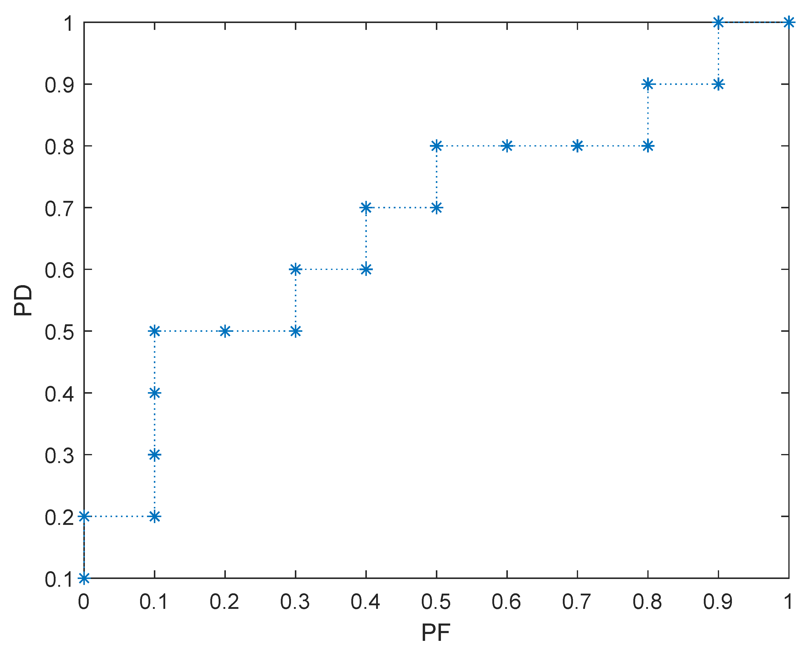
AUC is the area under of receiver operating characteristic (ROC) curve and ranges from 0 to 1, which is first used to evaluate the machine learning algorithm by Bradley [85]. The ROC curve is obtained by plotting PF on the X-axis and PD on the Y-axis. AUC is a widely used measure because it is rarely affected by class imbalance [82]. The AUC value of a random prediction model is 0.5. Given a testing dataset having 20 samples, the actual label and the scores, i.e., the predicted probability of being positive class, are shown in Table 3. In the table, P and N represent the positive and negative classes, respectively. We first sort scores in descending order and take each source as the threshold successively. For a sample, if its score is not smaller than threshold, then its label is predicted as positive class (i.e., P). For example, when the score of 3-th sample is used as the threshold, then both 1-th and 2-th samples are classified as positive class and the rest samples are predicted as negative class. For each threshold, we can construct a confusion matrix, as shown in Table 2, and then we can obtain a two-tuple of (PD and PF). Because the testing dataset has 20 samples, we can obtain 20 groups of (PD and PF). We then construct a two-dimensional (2-D) coordinate system where x-axis and y-axis present PF and PD, respectively. We plot 20 point of (PD and PF), then the ROC curve is obtained as Figure 1. As shown in the figure, the area under the ROC curve is called AUC whose value is equal to the sum of area of multiple rectangles under the curve. In this study, we directly use MATLAB build-in function perfcurve to calculate AUC.
4.4. Statistical Test
In this study, we use the Wilcoxon signed-rank test (at a significance level 0.05) in order to demonstrate whether our proposed CIB statistically outperforms the baselines on each dataset. The Wilcoxon signed-rank test is a non-parametric alternative to the paired t-test. Differing from the paired t-test, the Wilcoxon sighed-rank test does not assume that the samples must be normally distributed. Wilcoxon signed-rank test has been widely used in the previous SDP studies [21,89].
Moreover, Cliff’s [90] is used in order to further quantify the magnitude of difference, which is a non-parametric effect size measure. The magnitude is often assessed according to thresholds that are provided in by Romano et al. [91]: negligible (), small (), medium (), and large (). Cliff’s also has been widely used in the previous studies [13,87]. Cliff’s can be computed according to the method that was proposed by Macbeth et al. [92]. In this study, we use dark gray background cell ![Applsci 10 08059 i001]() to show that our CIB significantly outperforms the baseline with larger effect size, light gray cell
to show that our CIB significantly outperforms the baseline with larger effect size, light gray cell ![Applsci 10 08059 i002]() to show significant improvement with medium effect size, and silvery gray
to show significant improvement with medium effect size, and silvery gray ![Applsci 10 08059 i003]() to show significant improvement with small effect size.
to show significant improvement with small effect size.
 to show that our CIB significantly outperforms the baseline with larger effect size, light gray cell
  to show significant improvement with medium effect size, and silvery gray
  to show significant improvement with small effect size.
4.5. Experimental Settings
4.5.1. Validation Method
The k-fold cross-validation (CV) [93] is the most commonly used method for validating the prediction performance of SDP models in previous studies [60,94,95]. In this paper, 5-fold CV with 30 runs is used. Five-fold CV is used because of two main reasons: (1) software defect datasets are usually very imbalanced and too many folds are likely to result in the case that testing data has few defective samples. (2) it has been used in previous studies [60,95]. To alleviate possible sampling bias in random splits of CV, we repeat the five-fold CV process 30 times. 30 is used for the reason that it is the minimum needed samples to meet the central limit theory as done in [63].
Specifically, for a defect dataset, we randomly split it into five folds, which are approximately the same size and the same defective ratio. Additionally then, four folds are used as the training data and the reminding one fold is used as the test data. In this way, each fold has a chance to be taken as the test data. Then we take the average performance on the 5 different test data as the performance of a five-fold CV. Finally, we repeat above process 30 times and report the average performance on each dataset.
4.5.2. Parameter Settings
We set the maximum number of iterations T to 20 (see Line 10 in Algorithm 1), which is the same as that of three boosting related baselines, i.e., AdaC2, and AdaBoost. Because SMOTE is one step of our CIB, in this paper we just use WEKA data mining toolkit [96] to implement SMOTE, which has two key parameters: the percentage of synthetic minority class samples to generate P and the number of the nearest neighbors k. We let and , where and denote the number of majority class samples and the number of minority class samples for a given training dataset. The reason for setting is twofold: (1) it is the default value in WEKA, and (2) it was used by Chawla et al. [40] when they proposed the SMOTE algorithm. The reason for setting not a fixed value is that the value of P can be automatically adjusted according to the defect ratio of different defect datasets. Parameter in Equation (2) is set in order to make the value of equal to 0.9 when the , so as to make the credit factors of synthetic samples having two more real minority class samples be above 0.9.
With respect to the baselines, the settings follow the description of original studies if any, otherwise the default settings in the toolkit. The cost factor of AdaC2 is set to the imbalance ratio. The AdaBoost is implemented by WEKA in this paper and the parameter, i.e., the maximum number of iterations (i.e., T), is also set to 20. The reason for setting is that too small value may be unable take advantage of ensemble learning and too big value may cause over-fitting problem and be time-consuming. For baseline SMOTE, we also use the WEKA data mining toolkit [96] to implement it with the same setting as that in CIB. The number of removed majority class samples by RUS is equal to the difference between the number of majority class samples and that of minority class samples.
4.5.3. Base Classifier
In this paper, we consider C4.5 decision tree as the base classifier and implement it using the WEKA data mining toolkit [96].
J48 is a Java implementation of the C4.5 algorithm [97]. It uses the greedy technique for classification and generates decision trees, the nodes of which evaluate the existence or significance of individual features. Leaves in the tree structure represent classifications and branches represent the judging rules. It is easy to be transformed into a series of productive rules. One of the biggest advantages of decision tree is its good comprehensibility. Decision tree has been used as the base classifier in many previous studies [3,67].
5. Experimental Results
5.1. RQ1: How Effective Is CIB? How Much Improvement Can It Obtain Compared with the Baselines?
Table 4, Table 5, Table 6 and Table 7 respectively show the comparison results of F1, AGF, MCC, and AUC for our CIB and the baselines on each of 11 benchmark datasets. For each table, the best value on each data is highlighted in bold. The row ‘Average’ presents the average performance of each model across all benchmark datasets. The row ‘Win/Tie/Lose’ shows the comparison results of Wilcoxon signed-rank test (5%) when comparing our CIB with each baseline. Specifically, Win/Tie/Lose represents the number of datasets our CIB beats, ties with, or losses to the corresponding baseline, respectively. We use different background colors to show the results of effect size test (i.e., Cliff’s ). Specifically, the deep gray
![Applsci 10 08059 i004]() , the light gray
, the light gray ![Applsci 10 08059 i005]() , and the silvery gray
, and the silvery gray ![Applsci 10 08059 i006]() indicate that the proposed CIB significantly outperforms the corresponding baseline with large, moderate, and small effect size, respectively. If the baseline significantly outperforms our CIB or the effect size is negligible, then the corresponding table-cell of this baseline is marked with a white background. Checkmark ✓ represents that the corresponding method has no significant difference when compared with the best method.
indicate that the proposed CIB significantly outperforms the corresponding baseline with large, moderate, and small effect size, respectively. If the baseline significantly outperforms our CIB or the effect size is negligible, then the corresponding table-cell of this baseline is marked with a white background. Checkmark ✓ represents that the corresponding method has no significant difference when compared with the best method.
 , the light gray
  , and the silvery gray
  indicate that the proposed CIB significantly outperforms the corresponding baseline with large, moderate, and small effect size, respectively. If the baseline significantly outperforms our CIB or the effect size is negligible, then the corresponding table-cell of this baseline is marked with a white background. Checkmark ✓ represents that the corresponding method has no significant difference when compared with the best method.
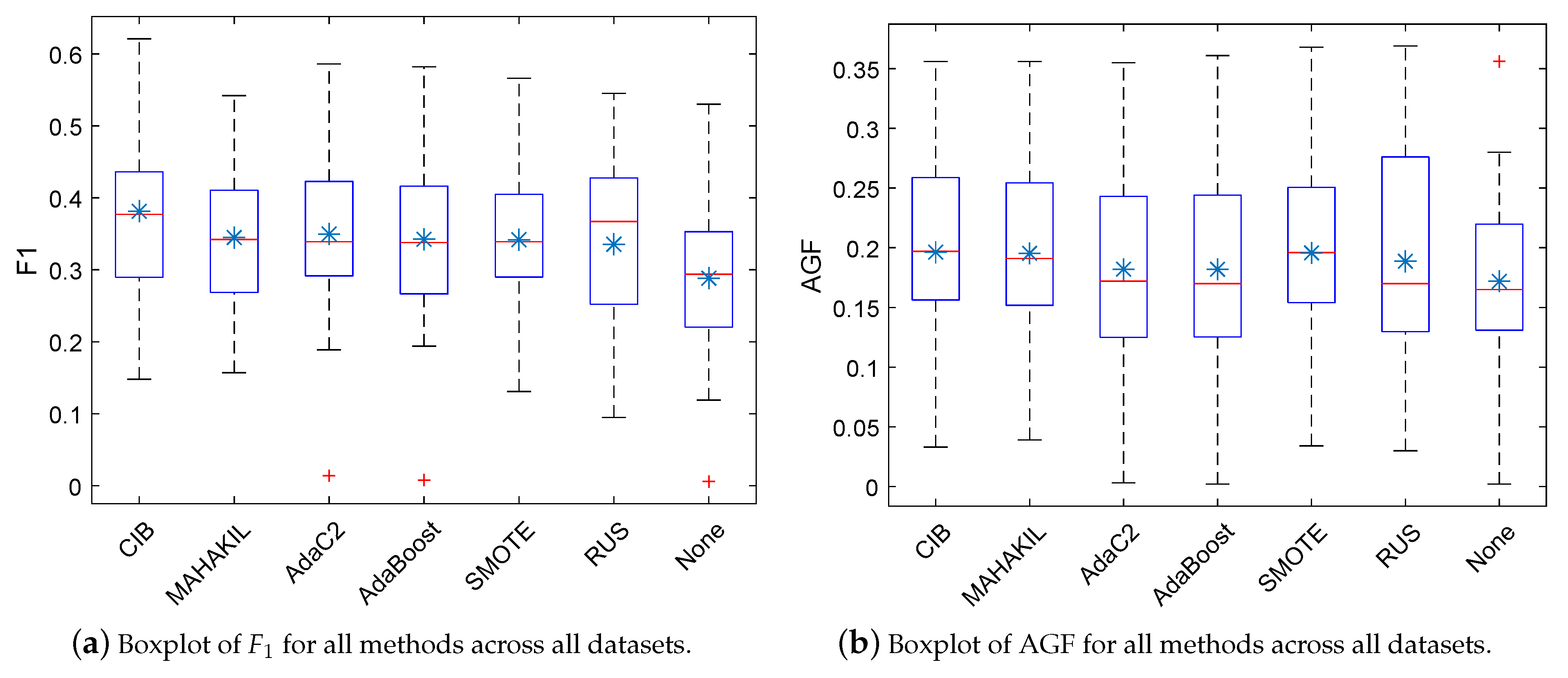
Figure 2a–d show the corresponding boxplots of F1, AGF, MCC, and AUC for all methods on 11 NASA datasets, where the horizontal line in the box denotes the median and the asterisk indicates the mean value. Table 8, Table 9, Table 10 and Table 11 separately present the 95% confidence interval of F1, AGF, MCC, and AUC for all methods on each of the 11 NASA datasets.
With respect to F1 (see Table 4), we notice that, on average, CIB obtains the best F1 as 0.381 across all datasets, which improves the performance over the baselines by at least 9% (see AdaC2 [45]). The F1 of CIB ranges from 0.148 (on dataset PC2) to 0.621 (on dataset PC4) across all 11 datasets. According to the results of ‘Win/Tie/Lose’ and the background of table cells, we notice that our CIB nearly always significantly outperforms AdaBoost and None with large effect size on all 11 datasets. Moreover, on most datasets, CIB significantly outperforms MAHAKIL, AdaC2, AdaBoost, and SMOTE with at least medium effect size and significantly perform worse than the baselines on at most one dataset.
With respect to AGF (see Table 5), we notice that, on average, CIB obtains the best AGF as 0.196 across all datasets, which is closely followed by SMOTE and MAHAKIL. The AGF of CIB ranges from 0.033 (on dataset MC1) to 0.356 (on dataset MC2) across all 11 datasets. According to the results of Wilcoxon signed-rank test (see the row ‘Win/Tie/Lose’) and the background of table cells, we notice that on most datasets, our CIB significantly outperforms AdaC2, AdaBoost, and None with large effect size on 11 datasets. Moreover, CIB has similar performance to SMOTE, MAHAKIL, and RUS.
With respect to MCC (see Table 6), we can see that, on average, CIB obtains the best MCC as 0.285, which improves the performance over the baselines by at least 3.7% (see AdaC2 [45]). The MCC of CIB ranges from 0.137 to 0.559 across all 11 datasets. According to the results of ‘Win/Tie/Lose’ and the background of table cells, we notice that CIB nearly always significantly outperforms None with a large effect size on all 11 datasets. On most datasets, our CIB significantly outperforms the remaining baselines including MAHAKIL, AdaC2, AdaBoost, SMOTE, and RUS with at least a medium effect size and significantly performs worse than the baselines on, at most, two datasets.
With respect to AUC (see Table 7), we can see that CIB achieves the biggest AUC as 0.769 on average, which improves the performance over the baselines by at least 1.2% (see AdaBoost [46]). The AUC of CIB ranges from 0.672 to 0.923 across all 11 datasets. According to the results of ‘Win/Tie/Lose’ and the background of table cells, we notice that our CIB always significantly outperforms MAHAKIL, SMOTE, RUS, and None with large effect size on each of 11 datasets. On at least half of 11 datasets, CIB significantly outperforms the remaining two baselines, i.e., AdaC2 and AdaBoost, with non-negligible effect size and has no significant differences with them on four out of 11 datasets.
Conclusion: on average, CIB always obtains the best performance in terms of F1, AGF, MCC, and AUC and improves F1/AGF/MCC/AUC over the baselines by at least 9%/0.2%/3.7%/1.2%. In most cases, our CIB significantly outperforms the baselines with at least medium effect size in terms of F1, MCC, and AUC.
5.2. RQ2: How Is the Generalization Ability of CIB?
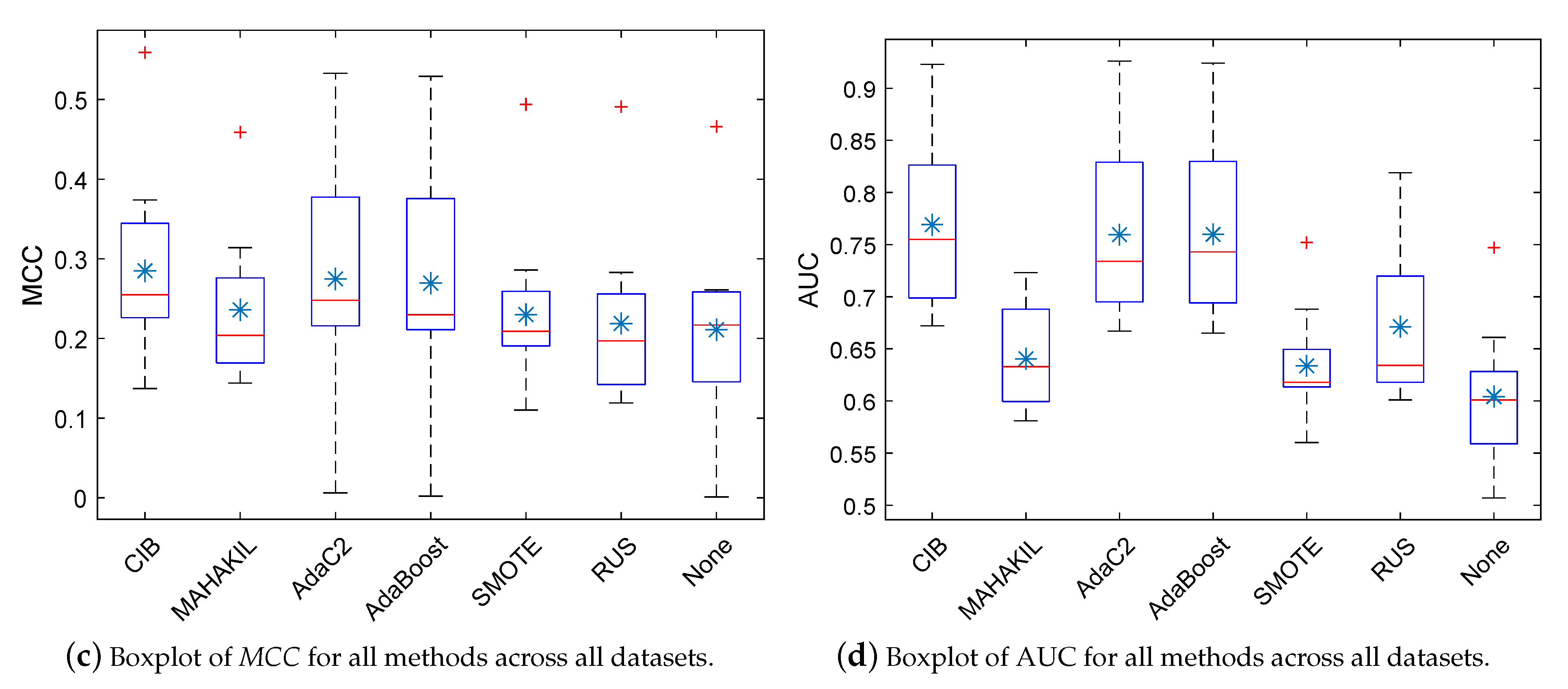
According to the experimental results on NASA datasets, we find that CIB is more promising to deal with the class-imbalance problem in SDP when compared with existing methods. Here, we want to investigate that whether the findings can be generalized to other scenarios, e.g., on other defect datasets. To this end, we compared CIB with the existing methods (see Section 4.2) on PROMISE datasets [43]. The PROMISE repository includes many defect datasets collected from open-source JAVA projects, such as camel, ant, etc. The details of nine PROMISE datasets are shown in Table 12. We take the same settings as Section 4.5. Due to the space limitation, we just report the experimental results of F1, AGF, AUC, and MCC with box plots as shown in the Figure 3.
From the figures, we can notice that CIB still outperforms all baselines in terms of F1, AGF, AUC, or MCC. Therefore, we can conclude that the findings have a good generalization.
5.3. RQ3: How Much Time Does It Take for CIB to Run?
To answer this question, we measure the training and testing time of CIB and the baselines. The training time includes the time taken for data preprocessing and model training. The testing time is the time that is taken to process the testing dataset until the value of performance measures is obtained.
Table 13 and Table 14 separately show the training and testing time of our CIB and the baselines. From the tables, we can see that (1) CIB needs the most training time and, on average, the training of CIB takes about 223.25 s; (2) the testing time of all methods is very small, on average, CIB takes 0.168 s in the testing. Therefore, we suggest that train CIB offline.
6. Discussion
6.1. Why CIB Works?
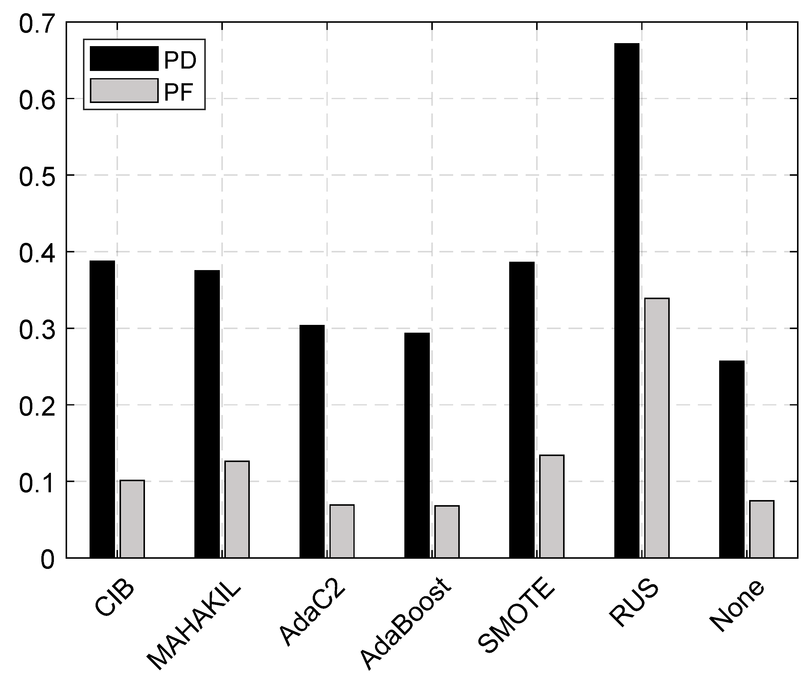
The experimental results provide substantial empirical support demonstrating that taking the credibility of synthetic samples into consideration is helpful for dealing with the class-imbalance problem in software defect prediction. The performance of CIB can be attributed to three aspects: oversampling, boosting framework, and the proposed credibility of synthetic samples. A good defect prediction model should have a high PD, but a low PF as Menzies [3] argued. We further empirically discuss how CIB works in terms of PD and PF.
Figure 4 presents the bar plots of PD and PF for CIB and the baselines across all 11 benchmark datasets. From the figure, we can see that RUS obtained the largest PD at the cost of a extremely high PF. The reason of high PF is that too mach useful information of non-defective samples is abandoned when randomly removing many non-defective samples, especially the case that the defect dataset is highly imbalanced. We also notice that CIB achieved the second largest PD (0.388), closely followed by SMOTE (PD = 0.386) and MAHAKIL (PD = 0.375) at the cost of a smaller PF than them. The reason of this is that some synthetic minority class samples generated by SMOTE are noisy, which damages the classification of actual majority class samples. When compared with AdaBoost, AdaC2, and None, CIB largely improved PD at the cost of an acceptable PF (PF = 0.101) considering that of AdaBoost (0.068), AdaC2 (PF = 0.069), and None (PF = 0.075).
In summary, any of CIB’s three components, including oversampling, boosting framework, and the proposed credibility of synthetic samples, is essential to ensure the performance of CIB.
6.2. Class-Imbalance Learning Is Necessary When Building Software Defect Prediction Models
The experimental results show that all class-imbalance learning methods are helpful to improve defect prediction performance in terms of F1, AGF, MCC, and AUC, which is consistent with the results of previous studies [40,44,45,46,64]. We also notice that, among all class-imbalance learning methods, CIB always makes the largest improvement over no class-imbalance learning method (i.e., None) in terms of F1, MCC, or AUC). Moreover, although RUS is the simplest class-imbalance learning method, it makes the smallest improvement over None in terms of F1 and MCC as compared with other class-imbalance learning methods. Therefore, users, who try to select a class-imbalance learning method to address the class-imbalance problem, should consider both the easy implementation and its actual performance. To sum up, CIB is a more promising alternative for addressing class-imbalance problem.
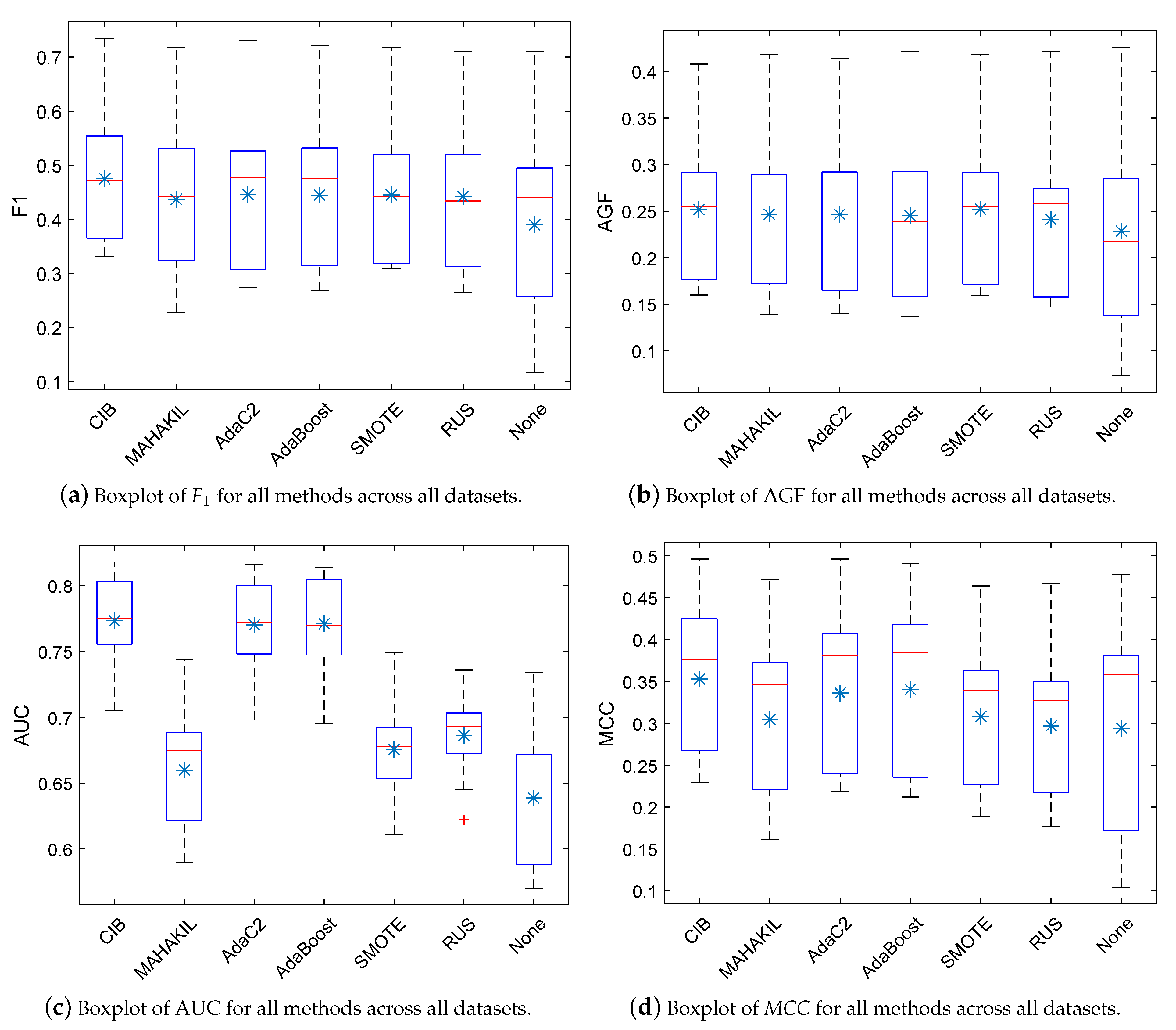
6.3. Is CIB Comparable to Rule-Based Classifiers?
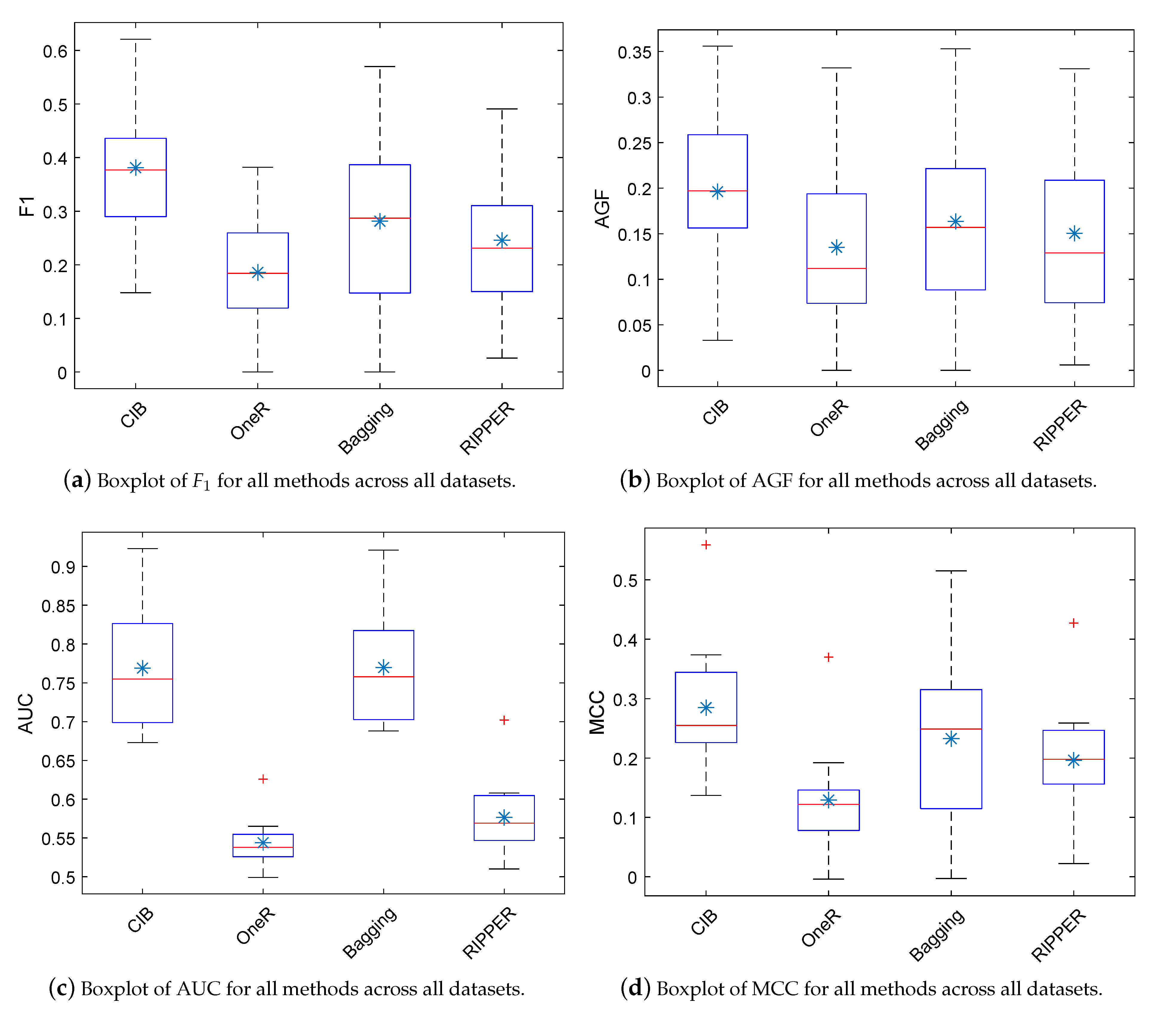
In this section, we provide a comparison between CIB and some rule-based classifiers, including OneR [98], Bagging (C4.5, i.e., J48, is used as the base classifier in this study) [99], and RIPPER [100]. We implement OneR, Bagging, and RIPPER by WEKA with the default parameters. We perform experiments on NASA datasets and use five-fold CV (see Section 4.5) to evaluate the prediction performance. On each dataset, we run each model 30 times with 5-fold CV and report the average performance. Owing to the space limitation, we just report the experimental results of F1, AGF, AUC, and MCC with box plots, as shown in the Figure 5.
From the figures, we can notice that (1), with respect to F1, AGF, and MCC, CIB obviously outperform the baselines, i.e., OneR, Bagging, and RIPPER; (2) with respect to AUC, CIB has similar performance to Bagging and obviously outperforms OneR and RIPPER.
6.4. Is CIB Applicable for Cross-Project Defect Prediction?
Honestly, we do not suggest directly using CIB for cross-project defect prediction (CPDP), because CIB is designed for addressing class-imbalance problem in within-project defect prediction (WPDP). As we all know that WPDP is completely different from CPDP. Therefore, the methods for WPDP are not suitable for addressing CPDP task. The biggest challenge in CPDP is the distribution difference between source and target datasets. CIB should be modified before using for cross-project defect prediction. To this end, for example, we can modify the method for calculating credit factor of synthetic minority class samples. The more the similarity between synthetic sample and the target dataset is, the bigger the credit factor of this synthetic sample. We plan to design a specific method to implement our idea in the future work.
6.5. Threats to Validity
External validity. In this paper, 11 NASA datasets are used as the benchmark datasets, which have been used in previous studies [3,27,67]. Moreover, we further discussed the performance of CIB on PROMISE datasets and obtain similar findings to that on NASA datasets. Honestly, we still cannot state that the same experimental conclusion can be obtained on other defect datasets. To alleviate this threat, the proposed CIB method should be applied to more defect datasets.
Construct validity. According to [101], different model validation techniques may affect model performance. Although the k-fold CV is one of the commonly used model validation techniques in previous studies [60,94,95], we still cannot ensure that our experimental results that are based on the 30*10-fold CV will be the same as that while using other validation techniques, e.g., hold-out validation technique. This could be a threat to the validity of our research.
Internal validity. Threats to internal validity mainly result from the re-implementation of the baseline methods and parameter tuning. Although we have carefully implemented the baselines and double-checked our source code, there may still be some mistakes in the code. In order to ensure the reliability of our research, the source code of our CIB and all baselines have been public on GitHub (https://github.com/THN-BUAA/CIB.git).
7. Conclusions
The class-imbalance data is a major factor to lower the performance of software defect prediction models [31,32]. Many class-imbalance learning methods have been proposed to address this problem in previous studies, especially the synthetic based oversampling methods, e.g., SMOTE [40]. Since previous synthetic based oversampling methods treat the artificial minority class samples equally with the real minority class samples, the unreliable synthetic minority samples may interfere the learning on real samples and shift the decision boundaries to incorrect directions. To address this limitation, we propose a credibility based imbalance boosting (CIB) method for software defect proneness prediction. To demonstrate the effectiveness of our CIB, experiments are conducted on 11 cleared NASA datasets and nine PROPMISE datasets. We compare CIB with previous class-imbalance learning methods, i.e., MAHAKIL [44], AdaC2 [45], AdaBoost [46], SMOTE [40] and RUS [35], in terms of three performance measures including AUC, F1, AGF, and MCC based on the well-known classifier (i.e., J48 decision tree). The experimental results show that our CIB is more effective compared with the baselines and is very promising to address the class-imbalance problem for software defect proneness prediction.
In the future, we plan to further demonstrate the effectiveness of our CIB on more defect datasets and modify CIB to use in cross-project defect prediction.
Author Contributions
Conceptualization, H.T. and S.W.; methodology, H.T.; data curation, G.L.; writing—original draft preparation, H.T.; writing—review and editing, H.T. and G.L.; supervision, S.W. All authors have read and agreed to the published version of the manuscript.
Funding
This work is funded by Field Fund of Equipment Development Department under grant #61400020404.
Acknowledgments
We would like to thank the editors and anonymous reviewers for their constructive comments and suggestions for the improvement of this paper.
Conflicts of Interest
We declare that we do not have any commercial or associative interest that represents a conflict of interest in connection with the work submitted.
Abbreviations
The following abbreviations are used in this manuscript:
| SDP | Software defect prediction |
| CIB | Credibility based imbalance boosting method |
| SOTA | State-of-the-art |
References
- Song, Q.; Jia, Z.; Shepperd, M.; Ying, S.; Liu, J. A General Software Defect-Proneness Prediction Framework. IEEE Trans. Softw. Eng. 2011, 37, 356–370. [Google Scholar] [CrossRef] [Green Version]
- Ostrand, T.J.; Weyuker, E.J.; Bell, R.M. Predicting the Location and Number of Faults in Large Software Systems. IEEE Trans. Softw. Eng. 2005, 31, 340–355. [Google Scholar] [CrossRef]
- Menzies, T.; Greenwald, J.; Frank, A. Data Mining Static Code Attributes to Learn Defect Predictors. IEEE Trans. Softw. Eng. 2007, 33, 2–13. [Google Scholar] [CrossRef]
- Gao, K.; Khoshgoftaar, T.M. A Comprehensive Empirical Study of Count Models for Software Fault Prediction. IEEE Trans. Reliab. 2007, 56, 223–236. [Google Scholar] [CrossRef]
- Shepperd, M.; Song, Q.; Sun, Z.; Mair, C. Data Quality: Some Comments on the NASA Software Defect Datasets. IEEE Trans. Softw. Eng. 2013, 39, 1208–1215. [Google Scholar] [CrossRef] [Green Version]
- Kamei, Y.; Shihab, E.; Adams, B.; Hassan, A.E.; Mockus, A.; Sinha, A.; Ubayashi, N. A Large-Scale Empirical Study of Just-in-Time Quality Assurance. IEEE Trans. Softw. Eng. 2013, 39, 757–773. [Google Scholar] [CrossRef]
- Catal, C. Software fault prediction: A literature review and current trends. Expert Syst. Appl. 2011, 38, 4626–4636. [Google Scholar] [CrossRef]
- Malhotra, R. An extensive analysis of search-based techniques for predicting defective classes. Comput. Electr. Eng. 2018, 71, 611–626. [Google Scholar] [CrossRef]
- McCabe, T.J. A Complexity Measure. IEEE Trans. Softw. Eng. 1976, SE-2, 308–320. [Google Scholar] [CrossRef]
- Halstead, M.H. Elements of Software Science; Elsevier Computer Science Library: Operational Programming Systems Series; North-Holland: New York, NY, USA, 1977. [Google Scholar]
- Kemerer, C.; Chidamber, S. A Metrics Suite for Object Oriented Design. IEEE Trans. Softw. Eng. 1994, 20, 476–493. [Google Scholar] [CrossRef] [Green Version]
- Madeyski, L.; Jureczko, M. Which process metrics can significantly improve defect prediction models? An empirical study. Softw. Qual. J. 2014, 1–30. [Google Scholar] [CrossRef] [Green Version]
- Yang, X.; Lo, D.; Xia, X.; Zhang, Y.; Sun, J. Deep Learning for Just-in-Time Defect Prediction. In Proceedings of the 2015 IEEE International Conference on Software Quality, Reliability and Security, Vancouver, BC, Canada, 3–5 August 2015; pp. 17–26. [Google Scholar] [CrossRef] [Green Version]
- Khoshgoftaar, T.M.; Allen, E.B.; Jones, W.D.; Hudepohl, J.I. Classification tree models of software quality over multiple releases. In Proceedings of the 10th International Symposium on Software Reliability Engineering (Cat. No.PR00443), Boca Raton, FL, USA, 1–4 November 1999; pp. 116–125. [Google Scholar] [CrossRef]
- Jin, C.; Jin, S.W. Prediction Approach of Software Fault-proneness Based on Hybrid Artificial Neural Network and Quantum Particle Swarm Optimization. Appl. Soft Comput. 2015, 35, 717–725. [Google Scholar] [CrossRef]
- Turhan, B.; Menzies, T.; Bener, A.B.; Di Stefano, J. On the relative value of cross-company and within-company data for defect prediction. Empir. Softw. Eng. 2009, 14, 540–578. [Google Scholar] [CrossRef] [Green Version]
- Miholca, D.L.; Czibula, G.; Czibula, I.G. A novel approach for software defect prediction through hybridizing gradual relational association rules with artificial neural networks. Inf. Sci. 2018, 441, 152–170. [Google Scholar] [CrossRef]
- Laradji, I.H.; Alshayeb, M.; Ghouti, L. Software defect prediction using ensemble learning on selected features. Inf. Softw. Technol. 2015, 58, 388–402. [Google Scholar] [CrossRef]
- Ryu, D.; Jang, J.I.; Baik, J. A Hybrid Instance Selection Using Nearest-Neighbor for Cross-Project Defect Prediction. J. Comput. Sci. Technol. 2015, 30, 969–980. [Google Scholar] [CrossRef]
- Ma, Y.; Luo, G.; Zeng, X.; Chen, A. Transfer learning for cross-company software defect prediction. Inf. Softw. Technol. 2012, 54, 248–256. [Google Scholar] [CrossRef]
- Xia, X.; Lo, D.; Pan, S.J.; Nagappan, N.; Wang, X. HYDRA: Massively Compositional Model for Cross-Project Defect Prediction. IEEE Trans. Softw. Eng. 2016, 42, 977–998. [Google Scholar] [CrossRef]
- Nam, J.; Pan, S.J.; Kim, S. Transfer defect learning. In Proceedings of the 2013 35th International Conference on Software Engineering (ICSE), San Francisco, CA, USA, 18–26 May 2013; pp. 382–391. [Google Scholar] [CrossRef]
- Wang, S.; Liu, T.; Tan, L. Automatically Learning Semantic Features for Defect Prediction. In Proceedings of the 38th International Conference on Software Engineering; ICSE ’16; ACM: New York, NY, USA, 2016; pp. 297–308. [Google Scholar] [CrossRef]
- Chen, L.; Fang, B.; Shang, Z.; Tang, Y. Negative samples reduction in cross-company software defects prediction. Inf. Softw. Technol. 2015, 62, 67–77. [Google Scholar] [CrossRef]
- Jing, X.; Wu, F.; Dong, X.; Qi, F.; Xu, B. Heterogeneous Cross-company Defect Prediction by Unified Metric Representation and CCA-based Transfer Learning. In Proceedings of the 2015 10th Joint Meeting on Foundations of Software Engineering; ESEC/FSE 2015; ACM: New York, NY, USA, 2015; pp. 496–507. [Google Scholar] [CrossRef]
- Li, Z.; Jing, X.Y.; Wu, F.; Zhu, X.; Xu, B.; Ying, S. Cost-sensitive transfer kernel canonical correlation analysis for heterogeneous defect prediction. Autom. Softw. Eng. 2018, 25, 201–245. [Google Scholar] [CrossRef]
- Nam, J.; Fu, W.; Kim, S.; Menzies, T.; Tan, L. Heterogeneous Defect Prediction. IEEE Trans. Softw. Eng. 2018, 44, 874–896. [Google Scholar] [CrossRef] [Green Version]
- Ryu, D.; Choi, O.; Baik, J. Value-cognitive Boosting with a Support Vector Machine for Cross-project Defect Prediction. Empir. Softw. Eng. 2016, 21, 43–71. [Google Scholar] [CrossRef]
- Hosseini, S.; Turhan, B.; Mäntylä, M. A benchmark study on the effectiveness of search-based data selection and feature selection for cross project defect prediction. Inf. Softw. Technol. 2018, 95, 296–312. [Google Scholar] [CrossRef] [Green Version]
- Boehm, B.; Basili, V.R. Software Defect Reduction Top 10 List. Computer 2001, 34, 135–137. [Google Scholar] [CrossRef]
- Hall, T.; Beecham, S.; Bowes, D.; Gray, D.; Counsell, S. A Systematic Literature Review on Fault Prediction Performance in Software Engineering. IEEE Trans. Softw. Eng. 2012, 38, 1276–1304. [Google Scholar] [CrossRef]
- Arisholm, E.; Briand, L.C.; Johannessen, E.B. A systematic and comprehensive investigation of methods to build and evaluate fault prediction models. J. Syst. Softw. 2010, 83, 2–17. [Google Scholar] [CrossRef]
- Pak, C.; Wang, T.T.; Su, X.H. An Empirical Study on Software Defect Prediction Using Over-Sampling by SMOTE. Int. J. Softw. Eng. Knowl. Eng. 2018, 28, 811–830. [Google Scholar] [CrossRef]
- Malhotra, R.; Khanna, M. An empirical study for software change prediction using imbalanced data. Empir. Softw. Eng. 2017, 22, 2806–2851. [Google Scholar] [CrossRef]
- He, Z.; Peters, F.; Menzies, T.; Yang, Y. Learning from open-source projects: An empirical study on defect prediction. In Proceedings of the 2013 ACM/IEEE International Symposium on Empirical Software Engineering and Measurement, Baltimore, MD, USA, 10–11 October 2013; pp. 45–54. [Google Scholar]
- Menzies, T.; Turhan, B.; Bener, A.; Gay, G.; Cukic, B.; Jiang, Y. Implications of Ceiling Effects in Defect Predictors. In Proceedings of the 4th International Workshop on Predictor Models in Software Engineering; PROMISE ’08; ACM: New York, NY, USA, 2008; pp. 47–54. [Google Scholar] [CrossRef] [Green Version]
- Khoshgoftaar, T.M.; Geleyn, E.; Nguyen, L.; Bullard, L. Cost-Sensitive Boosting in Software Quality Modeling. In Proceedings of the 7th IEEE International Symposium on High Assurance Systems Engineering; HASE ’02; IEEE Computer Society: Washington, DC, USA, 2002; pp. 51–60. [Google Scholar]
- Zheng, J. Cost-sensitive boosting neural networks for software defect prediction. Expert Syst. Appl. 2010, 37, 4537–4543. [Google Scholar] [CrossRef]
- Siers, M.J.; Islam, M.Z. Software defect prediction using a cost sensitive decision forest and voting, and a potential solution to the class imbalance problem. Inf. Syst. 2015, 51, 62–71. [Google Scholar] [CrossRef]
- Chawla, N.V.; Bowyer, K.W.; Hall, L.O.; Kegelmeyer, W.P. SMOTE: Synthetic Minority Over-sampling Technique. J. Artif. Int. Res. 2002, 16, 321–357. [Google Scholar] [CrossRef]
- Han, H.; Wang, W.Y.; Mao, B.H. Borderline-SMOTE: A New Over-Sampling Method in Imbalanced Data Sets Learning; Advances in Intelligent Computing ICIC 2005; Springer: Berlin/Heidelberg, Germany, 2005; Volume 3644, pp. 878–887. ISBN 978-3-540-28226-6. [Google Scholar]
- Barua, S.; Islam, M.M.; Yao, X.; Murase, K. MWMOTE-Majority weighted minority oversampling technique for imbalanced data set learning. IEEE Trans. Knowl. Data Eng. 2014, 26, 405–425. [Google Scholar] [CrossRef]
- Menzies, T.; Krishna, R.; Pryor, D. The Promise Repository of Empirical Software Engineering Data. 2015. Available online: http://openscience.us/repo (accessed on 10 October 2020).
- Ebo Bennin, K.; Keung, J.; Phannachitta, P.; Monden, A.; Mensah, S. MAHAKIL: Diversity Based Oversampling Approach to Alleviate the Class Imbalance Issue in Software Defect Prediction. IEEE Trans. Softw. Eng. 2017, 44, 534–550. [Google Scholar] [CrossRef]
- Sun, Y.; Kamel, M.S.; Wong, A.K.C.; Wang, Y. Cost-sensitive Boosting for Classification of Imbalanced Data. Pattern Recognit. 2007, 40, 3358–3378. [Google Scholar] [CrossRef]
- Freund, Y.; Schapire, R.E. A desicion-theoretic generalization of on-line learning and an application to boosting. In Computational Learning Theory; Vitányi, P., Ed.; Springer: Berlin, Germany, 1995; pp. 23–37. [Google Scholar]
- Wang, J.; Shen, B.; Chen, Y. Compressed C4. 5 models for software defect prediction. In Proceedings of the 2012 12th International Conference on Quality Software, Xi’an, China, 27–29 August 2012; pp. 13–16. [Google Scholar]
- Vashisht, V.; Lal, M.; Sureshchandar, G. Defect prediction framework using neural networks for software enhancement projects. J. Adv. Math. Comput. Sci. 2016, 16, 1–12. [Google Scholar] [CrossRef]
- Elish, K.O.; Elish, M.O. Predicting defect-prone software modules using support vector machines. J. Syst. Softw. 2008, 81, 649–660. [Google Scholar] [CrossRef]
- Okutan, A.; Yıldız, O.T. Software defect prediction using Bayesian networks. Empir. Softw. Eng. 2014, 19, 154–181. [Google Scholar] [CrossRef] [Green Version]
- Dejaeger, K.; Verbraken, T.; Baesens, B. Toward Comprehensible Software Fault Prediction Models Using Bayesian Network Classifiers. IEEE Trans. Softw. Eng. 2013, 39, 237–257. [Google Scholar] [CrossRef]
- Czibula, G.; Marian, Z.; Czibula, I.G. Software defect prediction using relational association rule mining. Inf. Sci. 2014, 264, 260–278. [Google Scholar] [CrossRef]
- Pan, C.; Lu, M.; Xu, B.; Gao, H. An Improved CNN Model for Within-Project Software Defect Prediction. Appl. Sci. Basel 2019, 9, 2138. [Google Scholar] [CrossRef] [Green Version]
- Shi, K.; Lu, Y.; Chang, J.; Wei, Z. PathPair2Vec: An AST path pair-based code representation method for defect prediction. J. Comput. Lang. 2020, 59, 100979. [Google Scholar] [CrossRef]
- Sun, Z.; Song, Q.; Zhu, X. Using Coding-Based Ensemble Learning to Improve Software Defect Prediction. IEEE Trans. Syst. Man Cybern. Part C Appl. Rev. 2012, 42, 1806–1817. [Google Scholar] [CrossRef]
- Khoshgoftaar, T.M.; Allen, E.B. Ordering Fault-Prone Software Modules. Softw. Qual. J. 2003, 11, 19–37. [Google Scholar] [CrossRef]
- Khoshgoftaar, T.; Gao, K.; Szabo, R.M. An Application of Zero-Inflated Poisson Regression for Software Fault Prediction. In Proceedings of the 12th International Symposium on Software Reliability Engineering; ISSRE ’01; IEEE Computer Society: Washington, DC, USA, 2001; pp. 66–73. [Google Scholar]
- Fagundes, R.A.A.; Souza, R.M.C.R.; Cysneiros, F.J.A. Zero-inflated prediction model in software-fault data. IET Softw. 2016, 10, 1–9. [Google Scholar] [CrossRef]
- Quah, T.S.; Thwin, M.M.T. Prediction of software development faults in PL/SQL files using neural network models. Inf. Softw. Technol. 2004, 46, 519–523. [Google Scholar] [CrossRef]
- Rathore, S.S.; Kumar, S. Linear and non-linear heterogeneous ensemble methods to predict the number of faults in software systems. Knowl.-Based Syst. 2017, 119, 232–256. [Google Scholar] [CrossRef]
- Mahmood, Z.; Bowes, D.; Lane, P.C.R.; Hall, T. What is the Impact of Imbalance on Software Defect Prediction Performance? In Proceedings of the 11th International Conference on Predictive Models and Data Analytics in Software Engineering; PROMISE ’15; ACM: New York, NY, USA, 2015; pp. 1–4. [Google Scholar] [CrossRef]
- Tantithamthavorn, C.; McIntosh, S.; Hassan, A.E.; Matsumoto, K. The Impact of Automated Parameter Optimization on Defect Prediction Models. IEEE Trans. Softw. Eng. 2019, 45, 683–711. [Google Scholar] [CrossRef] [Green Version]
- Krishna, R.; Menzies, T. Bellwethers: A Baseline Method For Transfer Learning. IEEE Trans. Softw. Eng. 2018. [Google Scholar] [CrossRef] [Green Version]
- Kamei, Y.; Monden, A.; Matsumoto, S.; Kakimoto, T.; Matsumoto, K. The Effects of Over and Under Sampling on Fault-prone Module Detection. In Proceedings of the First International Symposium on Empirical Software Engineering and Measurement (ESEM 2007), Madrid, Spain, 20–21 September 2007; pp. 196–204. [Google Scholar] [CrossRef]
- Seiffert, C.; Khoshgoftaar, T.M.; Van Hulse, J.; Folleco, A. An Empirical Study of the Classification Performance of Learners on Imbalanced and Noisy Software Quality Data. Inf. Sci. 2014, 259, 571–595. [Google Scholar] [CrossRef]
- Yang, X.; Lo, D.; Xia, X.; Sun, J. TLEL: A two-layer ensemble learning approach for just-in-time defect prediction. Inf. Softw. Technol. 2017, 87, 206–220. [Google Scholar] [CrossRef]
- Wang, S.; Yao, X. Using Class Imbalance Learning for Software Defect Prediction. IEEE Trans. Reliab. 2013, 62, 434–443. [Google Scholar] [CrossRef] [Green Version]
- Nguyen, G.H.; Bouzerdoum, A.; Phung, S.L. Learning Pattern Classification Tasks with Imbalanced Data Sets. Pattern Recognit. 2009, 193–208. [Google Scholar] [CrossRef] [Green Version]
- He, H.; Bai, Y.; Garcia, E.A.; Li, S. ADASYN: Adaptive synthetic sampling approach for imbalanced learning. In Proceedings of the 2008 IEEE International Joint Conference on Neural Networks (IEEE World Congress on Computational Intelligence), Hong Kong, China, 1–8 June 2008; pp. 1322–1328. [Google Scholar] [CrossRef] [Green Version]
- Ling, C.X.; Yang, Q.; Wang, J.; Zhang, S. Decision trees with minimal costs. In Proceedings of the Machine Learning, Proceedings of the Twenty-First International Conference (ICML 2004), Banff, AB, Canada, 4–8 July 2004. [Google Scholar] [CrossRef]
- Zhou, Z.H.; Liu, X.Y. Training Cost-Sensitive Neural Networks with Methods Addressing the Class Imbalance Problem. IEEE Trans. Knowl. Data Eng. 2006, 18, 63–77. [Google Scholar] [CrossRef]
- Khoshgoftaar, T.M.; Golawala, M.; Hulse, J.V. An Empirical Study of Learning from Imbalanced Data Using Random Forest. In Proceedings of the 19th IEEE International Conference on Tools with Artificial Intelligence(ICTAI 2007), Patras, Greece, 29–31 October 2007; Volume 2, pp. 310–317. [Google Scholar] [CrossRef]
- Fan, W.; Stolfo, S.J.; Zhang, J.; Chan, P.K. AdaCost: Misclassification Cost-Sensitive Boosting. In Proceedings of the Sixteenth International Conference on Machine Learning, ICML ’99, Bled, Slovenia, 27–30 June 1999; pp. 97–105. [Google Scholar]
- Chen, S.; He, H.; Garcia, E.A. RAMOBoost: Ranked minority oversampling in boosting. IEEE Trans. Neural Networks 2010, 21, 1624–1642. [Google Scholar] [CrossRef]
- Chawla, N.V.; Lazarevic, A.; Hall, L.O.; Bowyer, K.W. SMOTEBoost: Improving Prediction of the Minority Class in Boosting. In Knowledge Discovery in Databases; PKDD 2003; Springer: Berlin, Germany, 2003; pp. 107–119. [Google Scholar]
- Breiman, L. Random Forests. Mach. Learn. 2001, 45, 5–32. [Google Scholar] [CrossRef] [Green Version]
- Wohlin, C.; Runeson, P.; Höst, M.; Ohlsson, M.C.; Regnell, B.; Wesslén, A. Experimentation in Software Engineering; Springer: Berlin, Germany, 2012. [Google Scholar]
- Gray, D.; Bowes, D.; Davey, N.; Sun, Y.; Christianson, B. The misuse of the NASA metrics data program data sets for automated software defect prediction. In Proceedings of the 15th Annual Conference on Evaluation Assessment in Software Engineering (EASE 2011), Durham, UK, 11–12 April 2011; pp. 96–103. [Google Scholar] [CrossRef] [Green Version]
- Wu, X.; Kumar, V.; Quinlan, J.R.; Ghosh, J.; Yang, Q.; Motoda, H.; McLachlan, G.J.; Ng, A.; Liu, B.; Yu, P.S.; et al. Top 10 algorithms in data mining. Knowl. Inf. Syst. 2007, 14, 1–37. [Google Scholar] [CrossRef] [Green Version]
- Menzies, T.; Dekhtyar, A.; Distefano, J.; Greenwald, J. Problems with Precision: A Response to “comments on ‘data mining static code attributes to learn defect predictors’”. IEEE Trans. Softw. Eng. 2007, 33, 637–640. [Google Scholar] [CrossRef] [Green Version]
- Peters, F.; Menzies, T.; Gong, L.; Zhang, H. Balancing Privacy and Utility in Cross-Company Defect Prediction. IEEE Trans. Softw. Eng. 2013, 39, 1054–1068. [Google Scholar] [CrossRef] [Green Version]
- Tantithamthavorn, C.; Hassan, A.E.; Matsumoto, K. The Impact of Class Rebalancing Techniques on the Performance and Interpretation of Defect Prediction Models. IEEE Trans. Softw. Eng. 2018. [Google Scholar] [CrossRef] [Green Version]
- Bowes, D.; Hall, T.; Harman, M.; Jia, Y.; Sarro, F.; Wu, F. Mutation-aware Fault Prediction. In Proceedings of the 25th International Symposium on Software Testing and Analysis; ISSTA 2016; ACM: New York, NY, USA, 2016; pp. 330–341. [Google Scholar] [CrossRef] [Green Version]
- Maratea, A.; Petrosino, A.; Manzo, M. Adjusted F-measure and kernel scaling for imbalanced data learning. Inf. Sci. 2014, 257, 331–341. [Google Scholar] [CrossRef]
- Bradley, A.P. The Use of the Area Under the ROC Curve in the Evaluation of Machine Learning Algorithms. Pattern Recognit. 1997, 30, 1145–1159. [Google Scholar] [CrossRef] [Green Version]
- Matthews, B.W. Comparison of the predicted and observed secondary structure of T4 phage lysozyme. Biochim. Et Biophys. Acta 1975, 405, 442. [Google Scholar] [CrossRef]
- Zhang, F.; Mockus, A.; Keivanloo, I.; Zou, Y. Towards building a universal defect prediction model with rank transformed predictors. Empir. Softw. Eng. 2016, 21, 2107–2145. [Google Scholar] [CrossRef]
- Shepperd, M.; Bowes, D.; Hall, T. Researcher Bias: The Use of Machine Learning in Software Defect Prediction. IEEE Trans. Softw. Eng. 2014, 40, 603–616. [Google Scholar] [CrossRef] [Green Version]
- He, P.; Li, B.; Liu, X.; Chen, J.; Ma, Y. An Empirical Study on Software Defect Prediction with a Simplified Metric Set. Inf. Softw. Technol. 2015, 59, 170–190. [Google Scholar] [CrossRef] [Green Version]
- Cliff, N. Ordinal Methods for Behavioral Data Analysis; Psychology Press: New York, NY, USA, 1996. [Google Scholar]
- Romano, J.; Kromrey, J.D.; Coraggio, J.; Skowronek, J. Appropriate statistics for ordinal level data: Should we really be using t-test and Cohen’sd for evaluating group differences on the NSSE and other surveys. In Proceedings of the Annual Meeting of the Florida Association of Institutional Research, Tallahassee, FL, USA, 2–6 July 2006; pp. 1–33. [Google Scholar]
- Macbeth, G.; Razumiejczyk, E.; Ledesma, R. Cliff’s delta calculator: A non-parametric effect size program for two groups of observations. Univ. Psychol. 2011, 10, 545–555. [Google Scholar] [CrossRef]
- Hastie, T.; Tibshirani, R.; Friedman, J. The Elements of Statistical Learning: Data Mining, Inference, and Prediction; Springer: New York, NY, USA, 2009; pp. 241–247. [Google Scholar]
- Yu, X.; Liu, J.; Yang, Z.; Jia, X.; Ling, Q.; Ye, S. Learning from Imbalanced Data for Predicting the Number of Software Defects. In Proceedings of the 2017 IEEE 28th International Symposium on Software Reliability Engineering (ISSRE), Toulouse, France, 23–26 October 2017; pp. 78–89. [Google Scholar] [CrossRef]
- Chen, X.; Zhang, D.; Zhao, Y.; Cui, Z.; Ni, C. Software defect number prediction: Unsupervised vs supervised methods. Inf. Softw. Technol. 2019, 106, 161–181. [Google Scholar] [CrossRef]
- Frank, E.; Hall, M.A.; Witten, I.H. Data Mining: Practical Machine Learning Tools and Techniques, 4th ed.; Morgan Kaufmann: Burlington, MA, USA, 2016. [Google Scholar]
- Quinlan, J.R. C4.5: Programs for Machine Learning; Morgan Kaufmann Publishers Inc.: San Francisco, CA, USA, 1993. [Google Scholar]
- Challagulla, V.U.B.; Bastani, F.B.; Yen, I.-L.; Paul, R.A. Empirical assessment of machine learning based software defect prediction techniques. In Proceedings of the 10th IEEE International Workshop on Object-Oriented Real-Time Dependable Systems, Sedona, AZ, USA, 2–4 February 2005; pp. 263–270. [Google Scholar] [CrossRef]
- Shahrjooi Haghighi, A.; Abbasi Dezfuli, M.; Fakhrahmad, S. Applying Mining Schemes to Software Fault Prediction: A Proposed Approach Aimed at Test Cost Reduction. In Proceedings of the World Congress on Engineering (WCE 2012), London, UK, 4–6 July 2012; pp. 1–5. [Google Scholar]
- Cohen, W.W. Fast Effective Rule Induction. In Proceedings of the Twelfth International Conference on Machine Learning; Morgan Kaufmann: San Francisco, CA, USA, 1995; pp. 115–123. [Google Scholar]
- Tantithamthavorn, C.; McIntosh, S.; Hassan, A.E.; Matsumoto, K. An Empirical Comparison of Model Validation Techniques for Defect Prediction Models. IEEE Trans. Softw. Eng. 2017, 43, 1–18. [Google Scholar] [CrossRef]
Figure 1.
An example of ROC curve.

Figure 2.
Boxplot of F1, AGF, AUC, and MCC across all NASA datasets for our CIB and the baselines. The horizontal line in the box denotes the median and the asterisk indicates the mean value.
Figure 2.
Boxplot of F1, AGF, AUC, and MCC across all NASA datasets for our CIB and the baselines. The horizontal line in the box denotes the median and the asterisk indicates the mean value.


Figure 3.
Boxplot of F1, AGF, AUC, and MCC across all PROMISE datasets for our CIB and the baselines. The horizontal line in the box denotes the median and the asterisk indicates the mean value.
Figure 3.
Boxplot of F1, AGF, AUC, and MCC across all PROMISE datasets for our CIB and the baselines. The horizontal line in the box denotes the median and the asterisk indicates the mean value.

Figure 4.
Barplots of PD and PF for all methods across all benchmark datasets. The horizontal line in the box denotes the median, while the asterisk indicates the mean value.
Figure 4.
Barplots of PD and PF for all methods across all benchmark datasets. The horizontal line in the box denotes the median, while the asterisk indicates the mean value.

Figure 5.
Boxplot of F1, AGF, AUC, and MCC across all NASA datasets for our CIB and the baselines. The horizontal line in the box denotes the median, the asterisk indicates the mean value, and the red cross represents outliers.
Figure 5.
Boxplot of F1, AGF, AUC, and MCC across all NASA datasets for our CIB and the baselines. The horizontal line in the box denotes the median, the asterisk indicates the mean value, and the red cross represents outliers.


Table 1.
Statistics of 11 cleaned NASA datasets used in this study.
| Dataset | # of Metrics | # of Instances | # of Defective Instances | Defect Ratio |
|---|---|---|---|---|
| CM1 | 37 | 327 | 42 | 0.1284 |
| KC1 | 21 | 1183 | 314 | 0.2654 |
| KC3 | 39 | 194 | 36 | 0.1856 |
| MC1 | 38 | 1988 | 46 | 0.0231 |
| MC2 | 39 | 125 | 44 | 0.352 |
| MW1 | 37 | 253 | 27 | 0.1067 |
| PC1 | 37 | 705 | 61 | 0.0865 |
| PC2 | 36 | 745 | 16 | 0.0215 |
| PC3 | 37 | 1077 | 134 | 0.1244 |
| PC4 | 37 | 1287 | 177 | 0.1375 |
| JM1 | 21 | 7782 | 1672 | 0.2149 |
Table 2.
Confusion Matrix.
| Predicted | |||
|---|---|---|---|
| Positive | Negative | ||
| Actual | Positive | TP | FN |
| Negative | FP | TN | |
Table 3.
An example of a testing dataset along with the actual class label and scores (i.e., the predicted probability of being positive class).
Table 3.
An example of a testing dataset along with the actual class label and scores (i.e., the predicted probability of being positive class).
| No. | Class | Score | No. | Class | Score |
|---|---|---|---|---|---|
| 1 | P | 0.9 | 11 | P | 0.43 |
| 2 | P | 0.8 | 12 | N | 0.39 |
| 3 | N | 0.7 | 13 | P | 0.38 |
| 4 | P | 0.6 | 14 | N | 0.27 |
| 5 | N | 0.59 | 15 | N | 0.26 |
| 6 | P | 0.55 | 16 | N | 0.25 |
| 7 | N | 0.33 | 17 | P | 0.24 |
| 8 | N | 0.47 | 18 | N | 0.23 |
| 9 | P | 0.76 | 19 | N | 0.12 |
| 10 | N | 0.49 | 20 | N | 0.15 |
Table 4.
The comparison results of F1 for all methods in the form of mean ± standard deviation. The best value is in boldface.
Table 4.
The comparison results of F1 for all methods in the form of mean ± standard deviation. The best value is in boldface.
| Data | Our CIB | MAHAKIL [44] | AdaC2 [45] | AdaBoost [46] | SMOTE [40] | RUS [35] | None |
|---|---|---|---|---|---|---|---|
| CM1 | 28.3 ± 5.1✓ | 28.6 ± 5.1 | 18.9 ± 6.1 | 19.4 ± 5.5 | 30.8 ± 4.7 | 29.8 ± 3.7✓ | 20.4 ± 7.6 |
| KC1 | 44.3 ± 2.1 | 41.4 ± 1.9 | 42.6 ± 1.5 | 41.7 ± 1.8 | 40.6 ± 2.7 | 43.3 ± 2.2 ✓ | 35.6 ± 2.7 |
| KC3 | 40.4 ± 4.7 | 40.0 ± 5.7 ✓ | 32.6 ± 7.0 | 32.5 ± 5.9 | 40.2 ± 4.1 ✓ | 39.6 ± 5.6 ✓ | 34.4 ± 7.2 |
| MC1 | 23.8 ± 4.9 | 16.6 ± 4.8 | 41.3 ± 6.2 ✓ | 41.4 ± 6.9 | 13.1 ± 3.8 | 9.6 ± 1.1 | 11.9 ± 6.3 |
| MC2 | 58.2 ± 4.4 | 54.2 ± 4.6 | 55.8 ± 5.2 | 54.3 ± 5.8 | 50.4 ± 6.2 | 51.2 ± 6.0 | 46.6 ± 5.7 |
| MW1 | 31.0 ± 4.6 | 26.3 ± 6.0 | 30.0 ± 6.5 ✓ | 26.2 ± 7.1 | 28.4 ± 5.6 | 23.7 ± 3.6 | 29.4 ± 8.0 ✓ |
| PC1 | 41.5 ± 4.4 | 34.2 ± 3.4 | 40.7 ± 4.0 ✓ | 40.4 ± 5.4 ✓ | 35.0 ± 4.5 | 30.1 ± 2.2 | 30.7 ± 6.7 |
| PC2 | 14.8 ± 5.6 ✓ | 15.7 ± 7.8 | 1.4 ± 3.0 | 0.8 ± 2.4 | 13.3 ± 6.5 ✓ | 9.5 ± 1.4 | 0.6 ± 1.9 |
| PC3 | 37.7 ± 2.9 | 34.1 ± 2.8 | 28.9 ± 3.4 | 28.0 ± 3.0 | 33.7 ± 3.1 | 36.7 ± 2.2 ✓ | 27.0 ± 4.7 |
| PC4 | 62.1 ± 1.9 | 53.6 ± 2.2 | 58.6 ± 2.6 | 58.2 ± 2.4 | 56.6 ± 2.0 | 54.5 ± 1.5 | 53.0 ± 2.7 |
| JM1 | 37.4 ± 0.9 | 34.7 ± 1.2 | 33.9 ± 1.0 | 33.8 ± 0.7 | 33.9 ± 1.2 | 41.1 ± 0.5 | 27.6 ± 1.8 |
| Average | 38.1 | 34.5 | 35 | 34.2 | 34.2 | 33.6 | 28.8 |
| Improvement of Average | 10.6% | 9% | 11.4% | 11.6% | 13.7% | 32.3% | |
| Win/Tie/Lose | 8/3/0 | 8/2/1 | 9/1/1 | 8/3/0 | 6/4/1 | 10/1/0 | |
Note: (1) All numbers are in percentage (%) except the last two rows. (2) ✓ denotes the corresponding method has no significant difference with the best method. (3) ![Applsci 10 08059 i007]() ,
, ![Applsci 10 08059 i008]() , and
, and ![Applsci 10 08059 i009]() indicate that our CIB method significantly outperforms the corresponding baseline with large, moderate, and small effect size, respectively.
indicate that our CIB method significantly outperforms the corresponding baseline with large, moderate, and small effect size, respectively.
 ,
,  , and
, and  indicate that our CIB method significantly outperforms the corresponding baseline with large, moderate, and small effect size, respectively.
Table 5.
The comparison results of AGF for all methods in the form of mean ± standard deviation. The best value is in boldface.
Table 5.
The comparison results of AGF for all methods in the form of mean ± standard deviation. The best value is in boldface.
| Data | Our CIB | MAHAKIL [44] | AdaC2 [45] | AdaBoost [46] | SMOTE [40] | RUS [35] | None |
|---|---|---|---|---|---|---|---|
| CM1 | 17.5 ± 1.5 | 18.5 ± 1.3 ✓ | 12.0 ± 3.2 | 12.4 ± 2.9 | 19.0 ± 1.0 | 18.0 ± 1.9 | 12.9 ± 3.6 |
| KC1 | 31.4 ± 0.4 | 31.6 ± 0.4 | 30.7 ± 0.3 | 30.5 ± 0.4 | 30.9 ± 0.9 | 32.8 ± 0.8 | 28.0 ± 1.0 |
| KC3 | 23.4 ± 1.7 | 23.4 ± 1.9 ✓ | 20.3 ± 3.0 | 20.9 ± 2.6 | 23.4 ± 1.6 ✓ | 23.4 ± 1.7 ✓ | 21.1 ± 2.9 |
| MC1 | 6.5 ± 0.9 | 5.2 ± 1.2 | 7.7 ± 0.7 | 7.7 ± 0.7 ✓ | 5.1 ± 1.2 | 4.4 ± 0.6 | 3.3 ± 1.5 |
| MC2 | 35.6 ± 2.2 | 35.6 ± 3.0 ✓ | 35.5 ± 2.3 | 36.1 ± 1.5 ✓ | 36.8 ± 1.4 ✓ | 36.9 ± 3.4 | 35.6 ± 1.8 ✓ |
| MW1 | 15.5 ± 1.9 ✓ | 15.1 ± 2.1 ✓ | 14.0 ± 2.5 | 12.9 ± 2.9 | 15.3 ± 2.3 ✓ | 15.7 ± 2.1 | 13.7 ± 3.5 |
| PC1 | 16.0 ± 0.7 | 15.4 ± 0.8 | 15.7 ± 0.6 | 15.5 ± 1.0 | 15.7 ± 0.6 | 12.3 ± 1.8 | 14.3 ± 1.6 |
| PC2 | 3.3 ± 1.1 ✓ | 3.9 ± 1.8 | 0.3 ± 0.6 | 0.2 ± 0.5 | 3.4 ± 1.6 ✓ | 3.0 ± 1.1 | 0.2 ± 0.5 |
| PC3 | 19.7 ± 0.5 | 19.1 ± 0.8 | 17.2 ± 0.9 | 17.0 ± 0.8 | 19.6 ± 0.4 ✓ | 17.0 ± 1.4 | 16.5 ± 2.1 |
| PC4 | 20.2 ± 0.6 | 21.0 ± 0.5 | 21.6 ± 0.3 ✓ | 21.7 ± 0.2 | 20.5 ± 0.4 | 15.0 ± 1.5 | 21.3 ± 0.4 |
| JM1 | 26.7 ± 0.2 | 26.1 ± 0.4 | 25.2 ± 0.2 | 25.3 ± 0.2 | 25.6 ± 0.4 | 29.0 ± 0.1 | 22.2 ± 0.9 |
| Average | 19.6 | 19.5 | 18.2 | 18.2 | 19.6 | 18.9 | 17.2 |
| Improvement of Average | 0.4% | 7.8% | 7.8% | 0.2% | 4% | 14.1% | |
| Win/Tie/Lose | 4/4/3 | 8/1/2 | 8/1/2 | 4/4/3 | 4/4/3 | 9/1/1 | |
Note: (1) all numbers are in percentage (%) except the last two rows. (2) ✓ denotes the corresponding method has no significant difference with the best method. (3) ![Applsci 10 08059 i010]() ,
, ![Applsci 10 08059 i011]() , and
, and ![Applsci 10 08059 i012]() indicate our CIB method significantly outperforms the corresponding baseline with large, moderate, and small effect size, respectively.
indicate our CIB method significantly outperforms the corresponding baseline with large, moderate, and small effect size, respectively.
 ,
,  , and
, and  indicate our CIB method significantly outperforms the corresponding baseline with large, moderate, and small effect size, respectively.
Table 6.
The comparison results of MCC for all methods in the form of mean ± standard deviation. The best value is in boldface.
Table 6.
The comparison results of MCC for all methods in the form of mean ± standard deviation. The best value is in boldface.
| Data | Our CIB | MAHAKIL [44] | AdaC2 [45] | AdaBoost [46] | SMOTE [40] | RUS [35] | None |
|---|---|---|---|---|---|---|---|
| CM1 | 18.4 ± 5.6 ✓ | 16.9 ± 5.9 | 12.6 ± 6.7 | 13.7 ± 6.4 | 19.4 ± 5.7 | 17.3 ± 5.6 ✓ | 12.7 ± 7.7 |
| KC1 | 25.5 ± 2.7 ✓ | 20.4 ± 2.6 | 25.6 ± 2.0 | 24.7 ± 2.4 ✓ | 20.9 ± 2.7 | 17.7 ± 2.7 | 21.7 ± 2.5 |
| KC3 | 28.7 ± 6.1 | 27.0 ± 6.9 ✓ | 23.1 ± 8.4 | 23.0 ± 6.8 | 26.7 ± 5.2 ✓ | 23.2 ± 8.1 | 25.4 ± 8.5 ✓ |
| MC1 | 22.9 ± 4.8 | 15.8 ± 5.1 | 43.5 ± 5.9 ✓ | 44.0 ± 7.0 | 11.0 ± 4.0 | 12.8 ± 2.4 | 13.4 ± 7.7 |
| MC2 | 37.4 ± 6.9 | 31.4 ± 7.6 | 36.1 ± 8.3 ✓ | 34.5 ± 7.8 | 23.3 ± 8.4 | 21.1 ± 9.3 | 22.0 ± 8.3 |
| MW1 | 23.3 ± 5.3 | 17.0 ± 6.8 | 24.8 ± 7.2 ✓ | 21.4 ± 7.7 | 19.0 ± 6.4 | 11.9 ± 5.7 | 26.0 ± 8.7 |
| PC1 | 36.3 ± 4.8 | 27.8 ± 3.9 | 38.3 ± 4.4 ✓ | 38.6 ± 5.6 | 28.6 ± 5.2 | 26.4 ± 3.6 | 26.1 ± 6.8 |
| PC2 | 13.7 ± 6.0 ✓ | 14.4 ± 8.2 | 0.6 ± 3.3 | 0.2 ± 2.8 | 11.8 ± 7.1 ✓ | 13.2 ± 3.3 ✓ | 0.1 ± 2.0 |
| PC3 | 28.9 ± 3.3 | 24.3 ± 3.2 | 23.2 ± 3.7 | 22.4 ± 3.6 | 23.6 ± 3.6 | 28.3 ± 3.4 ✓ | 20.1 ± 4.2 |
| PC4 | 55.9 ± 2.2 | 45.9 ± 2.6 | 53.3 ± 2.9 | 52.9 ± 2.7 | 49.4 ± 2.3 | 49.1 ± 2.1 | 46.6 ± 2.9 |
| JM1 | 22.5 ± 1.0 | 18.7 ± 1.2 | 21.1 ± 1.1 | 21.0 ± 0.9 | 19.3 ± 1.2 | 19.7 ± 0.8 | 18.0 ± 1.1 |
| Average | 28.5 | 23.6 | 27.5 | 26.9 | 23 | 21.9 | 21.1 |
| Improvement of Average | 20.8% | 3.7% | 5.8% | 23.9% | 30.2% | 35.1% | |
| Win/Tie/Lose | 8/3/0 | 6/3/2 | 7/2/2 | 8/3/0 | 8/3/0 | 9/1/1 | |
Note: (1) all of the numbers are in percentage (%) except the last two rows. (2) ✓ denotes the corresponding method has no significant difference with the best method. (3) ![Applsci 10 08059 i013]() ,
, ![Applsci 10 08059 i014]() , and
, and ![Applsci 10 08059 i015]() indicate our CIB method significantly outperforms the corresponding baseline with large, moderate, and small effect size, respectively.
indicate our CIB method significantly outperforms the corresponding baseline with large, moderate, and small effect size, respectively.
 ,
,  , and
, and  indicate our CIB method significantly outperforms the corresponding baseline with large, moderate, and small effect size, respectively.
Table 7.
The comparison results of AUC for our CIB and the baselines in the form of mean ± standard deviation. The best value is in boldface.
Table 7.
The comparison results of AUC for our CIB and the baselines in the form of mean ± standard deviation. The best value is in boldface.
| Data | Our CIB | MAHAKIL [44] | AdaC2 [45] | AdaBoost [46] | SMOTE [40] | RUS [35] | None |
|---|---|---|---|---|---|---|---|
| CM1 | 72.7 ± 2.2 | 59.6 ± 4.4 | 73.4 ± 3.0 ✓ | 74.3 ± 3.4 | 61.3 ± 5.2 | 62.9 ± 4.1 | 55.0 ± 5.3 |
| KC1 | 67.8 ± 1.2 ✓ | 59.2 ± 2.2 | 68.1 ± 0.9 | 67.5 ± 1.5 ✓ | 60.2 ± 1.5 | 60.1 ± 1.6 | 58.6 ± 1.9 |
| KC3 | 72.2 ± 3.8 | 61.1 ± 5.8 | 69.5 ± 3.6 | 69.3 ± 3.4 | 61.7 ± 5.0 | 63.4 ± 6.1 | 58.9 ± 5.4 |
| MC1 | 83.3 ± 2.4 | 69.6 ± 4.6 | 85.7 ± 4.0 | 85.6 ± 3.3 ✓ | 65.8 ± 4.9 | 70.4 ± 4.3 | 60.1 ± 5.2 |
| MC2 | 75.5 ± 2.8 | 66.4 ± 4.6 | 73.9 ± 3.8 | 74.8 ± 4.0 ✓ | 61.5 ± 3.9 | 61.8 ± 5.9 | 61.4 ± 5.7 |
| MW1 | 69.1 ± 3.1 ✓ | 58.1 ± 6.6 | 69.5 ± 3.9 ✓ | 69.7 ± 2.6 | 62.4 ± 4.1 | 60.4 ± 5.0 | 54.5 ± 6.8 |
| PC1 | 85.9 ± 1.7 | 70.2 ± 4.2 | 84.0 ± 1.9 | 84.3 ± 2.1 | 68.8 ± 4.0 | 73.5 ± 3.5 | 66.1 ± 5.5 |
| PC2 | 79.4 ± 5.6 | 63.7 ± 10.1 | 72.4 ± 5.1 | 72.4 ± 4.9 | 56.0 ± 10.1 | 72.5 ± 4.7 | 50.7 ± 2.2 |
| PC3 | 80.6 ± 1.2 | 63.3 ± 2.9 | 79.6 ± 1.3 | 79.0 ± 1.3 | 61.8 ± 3.0 | 69.7 ± 3.1 | 63.3 ± 3.7 |
| PC4 | 92.3 ± 0.5 ✓ | 72.3 ± 2.3 | 92.6 ± 0.5 | 92.4 ± 0.6 ✓ | 75.2 ± 2.3 | 81.9 ± 1.8 | 74.7 ± 3.9 |
| JM1 | 67.2 ± 0.5 | 61.0 ± 0.8 | 66.7 ± 0.6 | 66.5 ± 0.5 | 62.3 ± 0.8 | 61.8 ± 0.7 | 61.4 ± 1.1 |
| Average | 76.9 | 64 | 75.9 | 76 | 63.4 | 67.1 | 60.4 |
| Improvement of Average | 20.1% | 1.3% | 1.2% | 21.4% | 14.6% | 27.3% | |
| Win/Tie/Lose | 11/0/0 | 6/4/1 | 5/4/2 | 11/0/0 | 11/0/0 | 11/0/0 | |
Note: (1) All numbers are in percentage (%) except the last two rows. (2) ✓ denotes the corresponding method has no significant difference with the best method. (3) ![Applsci 10 08059 i016]() ,
, ![Applsci 10 08059 i017]() , and
, and ![Applsci 10 08059 i018]() indicate our CIB method significantly outperforms the corresponding baseline with large, moderate, and small effect size, respectively.
indicate our CIB method significantly outperforms the corresponding baseline with large, moderate, and small effect size, respectively.
 ,
,  , and
, and  indicate our CIB method significantly outperforms the corresponding baseline with large, moderate, and small effect size, respectively.
Table 8.
95% confidence interval of F1 for CIB and the baselines on 11 NASA datasets.
| Data | Our CIB | MAHAKIL [44] | AdaC2 [45] | AdaBoost [46] | SMOTE [40] | RUS [35] | None |
|---|---|---|---|---|---|---|---|
| CM1 | [26.5, 30.1] | [26.8, 30.4] | [16.7, 21.1] | [17.4, 21.4] | [29.1, 32.5] | [28.5, 31.1] | [17.7, 23.1] |
| KC1 | [43.5, 45.1] | [41.0, 42.6] | [42.1, 43.1] | [41.1, 42.3] | [39.6, 41.6] | [42.5, 44.1] | [34.6, 36.6] |
| KC3 | [38.7, 42.1] | [38.0, 42.0] | [30.1, 35.1] | [30.4, 34.6] | [38.7, 41.7] | [37.6, 41.6] | [31.8, 37.0] |
| MC1 | [22.0, 25.6] | [14.9, 18.3] | [39.1, 43.5] | [38.9, 43.9] | [11.7, 14.5] | [9.2, 10.0] | [9.6, 14.2] |
| MC2 | [56.6, 59.8] | [52.6, 55.8] | [53.9, 57.7] | [52.2, 56.4] | [48.2, 52.6] | [49.1, 53.3] | [44.6, 48.6] |
| MW1 | [29.4, 32.6] | [24.3, 28.5] | [27.7, 32.3] | [23.7, 28.7] | [26.4, 30.4] | [22.4, 25.0] | [26.5, 32.3] |
| PC1 | [39.9, 43.1] | [31.8, 35.0] | [39.3, 42.1] | [38.5, 42.3] | [33.4, 36.6] | [29.3, 30.9] | [28.3, 33.1] |
| PC2 | [12.8, 16.8] | [12.9, 18.5] | [0.3, 2.5] | [−0.1, 1.7] | [11.0, 15.6] | [9.0, 10.0] | [−0.1, 1.3] |
| PC3 | [36.7, 38.7] | [31.4, 34.2] | [27.7, 30.1] | [26.9, 29.1] | [32.6, 34.8] | [35.9, 37.5] | [25.3, 28.7] |
| PC4 | [61.4, 62.8] | [52.7, 54.9] | [57.7, 59.5] | [57.3, 59.1] | [55.9, 57.3] | [54.0, 55.0] | [52.0, 54.0] |
| JM1 | [37.0, 37.8] | [33.7, 34.9] | [33.5, 34.3] | [33.7, 34.3] | [33.3, 34.5] | [40.7, 41.1] | [26.3, 27.9] |
Table 9.
95% confidence interval of AGF for CIB and the baselines on 11 NASA datasets.
| Data | Our CIB | MAHAKIL [44] | AdaC2 [45] | AdaBoost [46] | SMOTE [40] | RUS [35] | None |
|---|---|---|---|---|---|---|---|
| CM1 | [17.0, 18.0] | [18.0, 19.0] | [10.9, 13.1] | [11.4, 13.4] | [18.6, 19.4] | [17.3, 18.7] | [11.6, 14.2] |
| KC1 | [31.3, 31.5] | [31.5, 31.7] | [30.6, 30.8] | [30.4, 30.6] | [30.6, 31.2] | [32.5, 33.1] | [27.6, 28.4] |
| KC3 | [22.8, 24.0] | [22.7, 24.1] | [19.2, 21.4] | [20.0, 21.8] | [22.8, 24.0] | [22.8, 24.0] | [20.1, 22.1] |
| MC1 | [6.2, 6.8] | [4.8, 5.6] | [7.4, 8.0] | [7.4, 8.0] | [4.7, 5.5] | [4.2, 4.6] | [2.8, 3.8] |
| MC2 | [34.8, 36.4] | [34.5, 36.7] | [34.7, 36.3] | [35.6, 36.6] | [36.3, 37.3] | [35.7, 38.1] | [35.0, 36.2] |
| MW1 | [14.8, 16.2] | [14.3, 15.9] | [13.1, 14.9] | [11.9, 13.9] | [14.5, 16.1] | [14.9, 16.5] | [12.4, 15.0] |
| PC1 | [15.7, 16.3] | [15.1, 15.7] | [15.5, 15.9] | [15.1, 15.9] | [15.5, 15.9] | [11.7, 12.9] | [13.7, 14.9] |
| PC2 | [2.9, 3.7] | [3.3, 4.5] | [0.1, 0.5] | [0.0, 0.4] | [2.8, 4.0] | [2.6, 3.4] | [0.0, 0.4] |
| PC3 | [19.5, 19.9] | [18.8, 19.4] | [16.9, 17.5] | [16.7, 17.3] | [19.5, 19.7] | [16.5, 17.5] | [15.7, 17.3] |
| PC4 | [20.0, 20.4] | [20.8, 21.2] | [21.5, 21.7] | [21.6, 21.8] | [20.4, 20.6] | [14.5, 15.5] | [21.2, 21.4] |
| JM1 | [26.6, 26.8] | [25.9, 26.3] | [25.1, 25.3] | [25.2, 25.4] | [25.4, 25.8] | [29.0, 29.0] | [21.8, 22.6] |
Table 10.
95% confidence interval of MCC for CIB and the baselines on 11 NASA datasets.
| Data | Our CIB | MAHAKIL [44] | AdaC2 [45] | AdaBoost [46] | SMOTE [40] | RUS [35] | None |
|---|---|---|---|---|---|---|---|
| CM1 | [16.4, 20.4] | [14.8, 19.0] | [10.2, 15.0] | [11.4, 16.0] | [17.4, 21.4] | [15.3, 19.3] | [9.9, 15.5] |
| KC1 | [24.5, 26.5] | [19.6, 21.6] | [24.9, 26.3] | [23.8, 25.6] | [19.9, 21.9] | [16.7, 18.7] | [20.8, 22.6] |
| KC3 | [26.5, 30.9] | [24.5, 29.5] | [20.1, 26.1] | [20.6, 25.4] | [24.8, 28.6] | [20.3, 26.1] | [22.4, 28.4] |
| MC1 | [21.2, 24.6] | [14.0, 17.6] | [41.4, 45.6] | [41.5, 46.5] | [9.6, 12.4] | [11.9, 13.7] | [10.6, 16.2] |
| MC2 | [34.9, 39.9] | [28.7, 34.1] | [33.1, 39.1] | [31.7, 37.3] | [20.3, 26.3] | [17.8, 24.4] | [19.0, 25.0] |
| MW1 | [21.4, 25.2] | [14.7, 19.5] | [22.2, 27.4] | [18.6, 24.2] | [16.7, 21.3] | [9.9, 13.9] | [22.9, 29.1] |
| PC1 | [34.6, 38.0] | [25.2, 28.8] | [36.7, 39.9] | [36.6, 40.6] | [26.7, 30.5] | [25.1, 27.7] | [23.7, 28.5] |
| PC2 | [11.6, 15.8] | [11.5, 17.3] | [−0.6, 1.8] | [−0.8, 1.2] | [9.3, 14.3] | [12.0, 14.4] | [−0.6, 0.8] |
| PC3 | [27.7, 30.1] | [21.5, 24.5] | [21.9, 24.5] | [21.1, 23.7] | [22.3, 24.9] | [27.1, 29.5] | [18.6, 21.6] |
| PC4 | [55.1, 56.7] | [44.8, 47.4] | [52.3, 54.3] | [51.9, 53.9] | [48.6, 50.2] | [48.3, 49.9] | [45.6, 47.6] |
| JM1 | [22.1, 22.9] | [17.9, 19.1] | [20.6, 21.6] | [20.8, 21.6] | [18.9, 20.1] | [19.2, 20.0] | [17.2, 18.4] |
Table 11.
95% confidence interval of AUC for CIB and the baselines on 11 NASA datasets.
| Data | Our CIB | MAHAKIL [44] | AdaC2 [45] | AdaBoost [46] | SMOTE [40] | RUS [35] | None |
|---|---|---|---|---|---|---|---|
| CM1 | [71.9, 73.5] | [58.0, 61.2] | [72.3, 74.5] | [73.1, 75.5] | [59.4, 63.2] | [61.4, 64.4] | [53.1, 56.9] |
| KC1 | [67.4, 68.2] | [58.5, 59.7] | [67.8, 68.4] | [67.0, 68.0] | [59.7, 60.7] | [59.5, 60.7] | [57.9, 59.3] |
| KC3 | [70.8, 73.6] | [59.1, 63.3] | [68.2, 70.8] | [68.1, 70.5] | [59.9, 63.5] | [61.2, 65.6] | [57.0, 60.8] |
| MC1 | [82.4, 84.2] | [68.0, 71.2] | [84.3, 87.1] | [84.4, 86.8] | [64.0, 67.6] | [68.9, 71.9] | [58.2, 62.0] |
| MC2 | [74.5, 76.5] | [64.8, 68.0] | [72.5, 75.3] | [73.4, 76.2] | [60.1, 62.9] | [59.7, 63.9] | [59.4, 63.4] |
| MW1 | [68.0, 70.2] | [55.7, 60.5] | [68.1, 70.9] | [68.8, 70.6] | [60.9, 63.9] | [58.6, 62.2] | [52.1, 56.9] |
| PC1 | [85.3, 86.5] | [68.0, 71.6] | [83.3, 84.7] | [83.5, 85.1] | [67.4, 70.2] | [72.2, 74.8] | [64.1, 68.1] |
| PC2 | [77.4, 81.4] | [60.1, 67.3] | [70.6, 74.2] | [70.6, 74.2] | [52.4, 59.6] | [70.8, 74.2] | [49.9, 51.5] |
| PC3 | [80.2, 81.0] | [60.4, 63.4] | [79.1, 80.1] | [78.5, 79.5] | [60.7, 62.9] | [68.6, 70.8] | [62.0, 64.6] |
| PC4 | [92.1, 92.5] | [71.9, 73.9] | [92.4, 92.8] | [92.2, 92.6] | [74.4, 76.0] | [81.3, 82.5] | [73.3, 76.1] |
| JM1 | [67.1, 67.5] | [60.7, 61.5] | [66.4, 66.8] | [66.2, 66.8] | [61.9, 62.7] | [61.5, 62.1] | [60.8, 62.0] |
Table 12.
Statistics of PROMISE datasets used in this study.
| Dataset | # of Metrics | # of Instances | # of Defective Instances | Defect Ratio |
|---|---|---|---|---|
| ant-1.7 | 20 | 745 | 166 | 0.2228 |
| camel-1.6 | 20 | 965 | 188 | 0.1948 |
| ivy-2.0 | 20 | 352 | 40 | 0.1136 |
| jedit-4.1 | 20 | 312 | 79 | 0.2532 |
| log4j-1.0 | 20 | 135 | 34 | 0.2519 |
| prop-6 | 20 | 660 | 66 | 0.1 |
| tomcat | 20 | 858 | 77 | 0.0897 |
| xalan-2.6 | 20 | 885 | 411 | 0.4644 |
| xerces-1.3 | 20 | 453 | 69 | 0.1523 |
Table 13.
Training time of credibility based imbalance boosting (CIB) and the baselines (in second).
Table 13.
Training time of credibility based imbalance boosting (CIB) and the baselines (in second).
| Data | Our CIB | MAHAKIL [44] | AdaC2 [45] | AdaBoost [46] | SMOTE [40] | RUS [35] | None |
|---|---|---|---|---|---|---|---|
| CM1 | 11.05 | 2.2 | 0.53 | 0.23 | 0.38 | 0.03 | 0.02 |
| KC1 | 30.03 | 1.98 | 0.83 | 0.73 | 0.39 | 0.03 | 0.03 |
| KC3 | 3.52 | 0.56 | 0.25 | 0.17 | 0.2 | 0.02 | 0.01 |
| MC1 | 279.27 | 6.08 | 1.38 | 0.97 | 0.41 | 0.02 | 0.03 |
| MC2 | 2.11 | 0.36 | 0.22 | 0.06 | 0.22 | 0 | 0.01 |
| MW1 | 5.92 | 0.7 | 0.22 | 0.14 | 0.2 | 0 | 0.01 |
| PC1 | 31.56 | 2.16 | 0.52 | 0.38 | 0.23 | 0.02 | 0.01 |
| PC2 | 41.45 | 2.25 | 0.33 | 0.2 | 0.23 | 0 | 0.01 |
| PC3 | 64.95 | 2.83 | 0.88 | 0.83 | 0.28 | 0.02 | 0.03 |
| PC4 | 87 | 3.14 | 0.86 | 0.83 | 0.42 | 0.03 | 0.07 |
| JM1 | 1898.88 | 10.11 | 14.59 | 10.94 | 1.84 | 0.28 | 0.31 |
| Average | 223.25 | 2.94 | 1.87 | 1.41 | 0.44 | 0.04 | 0.05 |
Table 14.
Testing time of CIB and the baselines (in second).
| Data | Our CIB | MAHAKIL [44] | AdaC2 [45] | AdaBoost [46] | SMOTE [40] | RUS [35] | None |
|---|---|---|---|---|---|---|---|
| CM1 | 0.203 | 0.219 | 0.203 | 0.266 | 0.156 | 0.313 | 0.225 |
| KC1 | 0.188 | 0.172 | 0.141 | 0.125 | 0.406 | 0.109 | 0.127 |
| KC3 | 0.141 | 0.094 | 0.125 | 0.125 | 0.188 | 0.172 | 0.134 |
| MC1 | 0.172 | 0.078 | 0.172 | 0.109 | 0.172 | 0.141 | 0.122 |
| MC2 | 0.141 | 0.078 | 0.172 | 0.109 | 0.125 | 0.141 | 0.112 |
| MW1 | 0.141 | 0.109 | 0.141 | 0.172 | 0.172 | 0.156 | 0.162 |
| PC1 | 0.156 | 0.078 | 0.156 | 0.172 | 0.141 | 0.125 | 0.119 |
| PC2 | 0.188 | 0.094 | 0.156 | 0.125 | 0.125 | 0.203 | 0.158 |
| PC3 | 0.141 | 0.094 | 0.125 | 0.125 | 0.125 | 0.125 | 0.139 |
| PC4 | 0.141 | 0.078 | 0.141 | 0.156 | 0.141 | 0.156 | 0.127 |
| JM1 | 0.234 | 0.094 | 0.141 | 0.172 | 0.234 | 0.125 | 0.115 |
| Average | 0.168 | 0.108 | 0.152 | 0.151 | 0.18 | 0.161 | 0.14 |
Publisher’s Note: MDPI stays neutral with regard to jurisdictional claims in published maps and institutional affiliations. |
© 2020 by the authors. Licensee MDPI, Basel, Switzerland. This article is an open access article distributed under the terms and conditions of the Creative Commons Attribution (CC BY) license (http://creativecommons.org/licenses/by/4.0/).
Share and Cite
MDPI and ACS Style
Tong, H.; Wang, S.; Li, G. Credibility Based Imbalance Boosting Method for Software Defect Proneness Prediction. Appl. Sci. 2020, 10, 8059. https://0-doi-org.brum.beds.ac.uk/10.3390/app10228059
AMA Style
Tong H, Wang S, Li G. Credibility Based Imbalance Boosting Method for Software Defect Proneness Prediction. Applied Sciences. 2020; 10(22):8059. https://0-doi-org.brum.beds.ac.uk/10.3390/app10228059
Chicago/Turabian StyleTong, Haonan, Shihai Wang, and Guangling Li. 2020. "Credibility Based Imbalance Boosting Method for Software Defect Proneness Prediction" Applied Sciences 10, no. 22: 8059. https://0-doi-org.brum.beds.ac.uk/10.3390/app10228059
Note that from the first issue of 2016, this journal uses article numbers instead of page numbers. See further details here.