Automatic Colorization of Anime Style Illustrations Using a Two-Stage Generator


1
Department of AI Convergence Engineering, Gyeongsang National University, Jinjudaero 501, Jinju, Korea
2
Department of Aerospace and Software Engineering, Gyeongsang National University, Jinjudaero 501, Jinju, Korea
*
Author to whom correspondence should be addressed.
Appl. Sci. 2020, 10(23), 8699; https://0-doi-org.brum.beds.ac.uk/10.3390/app10238699
Submission received: 5 November 2020
/
Revised: 30 November 2020
/
Accepted: 2 December 2020
/
Published: 4 December 2020
(This article belongs to the Special Issue Artificial Intelligence and Machine Learning in Software Engineering)
Abstract
:Featured Application
Colorization of line-arts in storyboards for media industries including movie, animation, and game. Automatic colorization of comic strips, anime style images, and cartoons.
Abstract
Line-arts are used in many ways in the media industry. However, line-art colorization is tedious, labor-intensive, and time consuming. For such reasons, a Generative Adversarial Network (GAN)-based image-to-image colorization method has received much attention because of its promising results. In this paper, we propose to use color a point hinting method with two GAN-based generators used for enhancing the image quality. To improve the coloring performance of drawing with various line styles, generator takes account of the loss of the line-art. We propose a Line Detection Model (LDM) which is used in measuring line loss. LDM is a method of extracting line from a color image. We also propose histogram equalizer in the input line-art to generalize the distribution of line styles. This approach allows the generalization of the distribution of line style without increasing the complexity of inference stage. In addition, we propose seven segment hint pointing constraints to evaluate the colorization performance of the model with Fréchet Inception Distance (FID) score. We present visual and qualitative evaluations of the proposed methods. The result shows that using histogram equalization and LDM enabled line loss exhibits the best result. The Base model with XDoG (eXtended Difference-Of-Gaussians)generated line-art with and without color hints exhibits FID for colorized images score of 35.83 and 44.70, respectively, whereas the proposed model in the same scenario exhibits 32.16 and 39.77, respectively.
1. Introduction
Line-artworks play a crucial role in the initial phases of media industries for making storyboards, games, illustrations, animations, and movies. Since there is a limit in communicating the complicated emotional transitions and atmosphere of a scene using only line-art, it is a customary to use colorized line-art and colorful storyboards to convey ideas. However, coloring line-art is a very tedious and manual labor intensive job. For example, if an animation is two hours long and uses 24 frames per second, then animators have to colorize about 17 thousand frames. If we assume that colorization of line-art takes about 5 min per frame then it would take about 2302 days of working hours without any resting. To automate the colorization of line-art, the research community began to use Generative Adversarial Networks (GANs) [1]. There are also commercialized tools such as PaintsChainer and Clips Studio that automate the line-art; however, the perceived quality of the results are not as satisfactory as real-world colorized line-arts.
Colorization of line-arts are considered as difficult because, unlike black and white images, it does not contain texture or shade information. Although many models make use of a reference image or add few hint pixels on a line-art to aid the colorization process, the result of colorization shows limited color spectrum and monotonous color space. Basic steps included in automatic colorization of line-art are acquiring characteristics or features from a line-art, segmenting the image to generate texture and shades from a limited information, and seamlessly concatenating the segments as a final colorized image.
The automatic colorization of line-art can be categorized into three depending on the types of input data. The first category is fully automatic colorization that exploits only the line-art [2,3]. The second category is semi-automatic colorization which makes use of style transfer based on input data of line-arts and colorized images [4,5,6]. The final category is hint-based methods that inform what color to be used in which specific area of an image [7,8,9,10,11,12].
All three categories of colorization models have to extract contour of lines from the original line-art. Interestingly, the colorization performance of a generated colored line-art of the artificial line is better than that of real-world line-arts drawn by a artist. We conjecture that the low quality is due to over-fitting of input line-art data and imbalance of distribution of input line style and the distribution of real-world line style. In this work, we provide solution to over-fitting of the line style distribution and colorize a line-art with better color spectrum, shades, and gradation.
The proposed scheme is composed of five steps: (1) line-art augmentation with histogram equalization, (2) conversion of original image to grayscale image for subset of line-art, (3) data augmentation with two different line extraction method, (4) Line Detection Model (LDM) loss function for line generalization, and (5) two-stage generator that takes a low resolution image in the draft model and enhances color quality in the colorization stage. Figure 1 shows the result of colored images exploiting the proposed method using real-world images as the input data.
Many of the works in the field have used Fréchet Inception Distance (FID) score to compare the quality of generated images. However, we believe that simple FID score does not provide a fair comparison in the field of colorization because the generated color spectra are not correlated across the generated images. In this paper, we propose segment-based hinting constraints for consistent and fair comparison of colorized artworks. We named this method as Colorization FID (C-FID). We have conducted C-FID evaluation on the proposed model with XDoG generated line-art and real-world line-arts. When we provided a weak hint with 28 pixels on artificial line-art and real-world line-art, the FID shows 32.16 and 57.51 in the proposed model which are the lowest, respectively. In the case of FID measured on the artificial line-art and original line-art without hints, the result shows 39.77 and 98.75, respectively.
The main contributions of the work are as follows:
- Provide flexibility in enhancing the resolution of an image through two stage generators.
- Introduction of line style distribution generalization via histogram equalization of line-art to provide better colorization performance.
- Randomly use the grayscale transformed image instead of the line-art in data augmentation to increase the line-art generalization performance.
- Introduction of seven segment hint pointing constraints in measuring the performance of line-art colorization.
The organization of the paper is as follows. Section 2 introduces the research done on the field of colorization of line-arts. Section 3 describes the proposed data augmentation method, construction of model, and learning method. Section 4 explains the data used in the learning, presents result of experiments, and analyzes the result. Finally, Section 5 concludes the paper.
2. Related Work
In this section, we describe GAN- and Convolutional Neural Network (CNN)-based methods in the colorization of line-arts. There are three different methods (fully automatic colorization, style transfer or semi automatic colorization, and user hint) of colorization the line-art with respect to input data format.
2.1. Generative Adversarial Networks
Recently, Generative Adversarial Network (GAN) model [1] is proven to be efficient in generating super resolution image [13], Text To Speech (TTS) [14], and data augmentation [15] because of its performance in generating high quality data. GAN is composed of generator that generates data similar to the real data and discriminator that tries to distinguished the generated data among the real data. The goal of the two models is to deceive the other model. As a result, generator model generates a data that closely follows the distribution of input data.
Despite the advantages of GAN model, it is not a trivial job to balance the training of the two models. Moreover, it is also very difficult to have control over the output of GAN model because the output follows the distribution of input data. After numerous experiments, Radford et al. [16] proposed Deep Convolutional Generative Adversarial Network (DCGAN) that exploits CNN and batch normalization [17] in building balanced generator and discriminator model structure. Mehdi et al. [18] proposed Conditional GAN (cGAN) that employs class labels to have control over generated data.
2.2. Fully Automatic Colorization
Fully automated line-art colorization uses only the line-art without any other form of user aids [2,3]. Isola et al. [2] (Pix2Pix) used the Conditional GAN model to provide solution to image-to-image translation problems. By combining the adversarial loss and the loss, they create a photo realistic image. Kang et al. [3] used three different models (low resolution painter, background detector, and polishing network) to colorize the line-art. Low resolution painter model colors the given line-art. Background detector model distinguishes the foreground and the background of the line-art. Polishing network model combines the resulting low resolution image and extracted background segments to restore the resolution of the image. By exploiting the characteristics of speech bubbles in comics, they filled in the speech bubble regardless of the non image components such as letters in the comic. Although they show superior quality in preventing background color bleeding, they lack in power in painting a specific location with a certain color. Another issue with it is that the output resolution of the image is limited to 256 × 256 pixels.
2.3. Style Transfer-Based Colorization
Another way of automatically colorizing the line-art is based on style transfers [4,5,6]. It makes use of two user input data consisting line-art and colored image as a reference style. Furusawa et al. [4] exploit a reference image and interactive color hint (color palette) on comic strips to allow users to have control over the choice of color within the line-art. They synthesized coloring information acquired in colorization process onto contour information from the original comic strip. Although the use of color palette gives better control over the chosen color in a specific area of the image, the colors are painted or spread over the contour and the letters. Another issue with synthesizing is that the contours can not be clearly extracted from the image; as a result, intended texture is incompletely blended into the image. Zhang et al. [6] exploit style image through VGG16/19 model network. They introduced two guide decoder within the model to prevent the vanishing gradient and achieve better quality of colorized artwork. However, since they use VGG16/19 network model, it contains multiple issues. the first issue is that the size of the model is large; second, it is difficult to have control over colors in specific area; and lastly, the resolution of the final image is limited to 256 × 256 pixels.
2.4. Colorization with Color Point Hinting
The third type of automatic colorization of line-art exploits user provided hint to paint certain color in specific areas of the image [7,8,9,10,11,12]. A representative work on this category is done by Ci et al. [10]. They used Local Feature Network (LFN) to prevent the over-fitting of artificially generated lines from. They claim that the use of LFN in their approach has solved the issue of the over-fitting of lines in the image through generalization of lines. One disadvantage is that they exploit VGG16 in calculating loss of the model, which results in large model size. Sangkloy et al. [7] made use of four different line extraction methods to prevent over-fitting in painting face line-art. Frans et al. [9] exploited two separate generators for learning colors and shades. Liu et al. [8] devised a way to reduce the color smearing or spilling over the contour through maneuvering coefficients of loss. The result of their work shows better image quality than Pix2pix [2]. Hati et al. [12] also used a two-stage generator. The colorization model is based on generator model proposed by Ci et al. [10]. The colorization model generates an image and the line model generates artificial line-art from the provided image. They increased the colorization performance by taking account of reconstruction loss of generated line-art and real-world line-arts in colorization model. Zhang et al. [11] tried to improve the performance of colorization via exploiting two stage generator model. They reduce the dependency of initial image in post processing model by stimulating artifacts in the generated draft image.
3. Structure of Proposed Method
The overall layout of the proposed system is illustrated in Figure 2. It uses two generators (draft model and colorization model). The first generator creates a roughly colored draft image (128 × 128). The second generator enhances the image generated in the draft model, then increases its dimension to 512 × 512. To generate the colorized image, two models learn the provided line-art and a weak hint. Section 3.1 and Section 3.2 describe the method used in the pre-processing and Line Detection Model used in the learning of the draft stage, respectively. In Section 3.3, we define and explain the image generator model used in the colorization stage. Section 3.4 describes the classifier used in GAN, and Section 3.5 describes the loss functions used in the models.
3.1. Line-Art Over-Fitting
To paint the line-art, existing works exploit a pair of line-art and color image. In order to obtain contour of lines from an image, one needs to manually select the lines which takes a long laborious time even for experienced artisans. Thus, the research community moved on to self-learning-based methods where computer vision algorithms are used to extract contours of lines in an original colorized image and exploit them in the learning process. The colorization performance of generated line-arts and real-world line-arts are quite different. However, the colorization performance of actual line-art tends to be low. The reason for the low performance is overfitting of line distribution. The pixel distribution of real-world images and algorithmically extracted lines from color image is different. By learning the inaccurate line distribution, we cannot achieve good colorization performance. Ci et al. [10] tried to solve the over-fitting problem using LFN that has pre-trained by animation illustrations and tags. In the case of the model proposed by Ci et al. [10], they have to use LFN in the inference stage. Sangkloy et al. [7], on the other hand, approached the over-fitting of lines in different angle. They exploit four different methods to extract the artificial contour of lines and use them as data samples to learn to produce generalized line-arts.
In this work, we propose to increase the level of generalization of artificial lines used in the learning through following four techniques. First, the use of auto-encoder that extracts lines from a colorized image as a transfer learning model for draft model. Second, a subset of images are converted to grayscale image. Then, they are used as the line-art for learning. Third, one of the two artificial line generation scheme is randomly chosen to generate lines with diverse line distribution. Fourth, use of histogram equalizer to generalize lines and augmentation of samples.
Depending on the algorithms used for line extraction, the histogram of lines can be very different. Figure 3 shows the histogram of two different line extraction methods and a real-world line-arts. Figure 4 shows the image after applying the line extraction methods. We can observe that histogram of real-world line-arts are densely populated from 0 to about 170 where as XDoG and Dilate abs sub covers about 120 to 140 and about 0 to 60, respectively. The difference in line style distribution can be seen clearly in Figure 4. The distribution can also be affected by characteristics of digitizer pen, parameters used for image editors such as pen style, padding, style, and pen pressure. Although not shown in the paper, our initial experiment shows that the stability of the colorization of an image is very sensitive to the brightness of the line. Combining all the test results, we deduce that the quality of colorization of line-art depends on the distribution of line style.
In this work, histogram equalization is applied on the brightness of lines to generalize line style of an image. During the pre-process stage of the learning, we convert a line-art to grayscale and then apply histogram equalizer on that image to augment the learning data. One side effect of using histogram equalization is that it is a lossy transformation that changes the average brightness of lines. In our case, the histogram equalization is only applied in the pre-processing stage and a new information is generated in the draft generation, thus the characteristic of the line remains the same.
3.2. Pre-Processing
Data used in the learning phase are a pair of extracted line-art and the color image cropped in the dimension of 512 × 512 at a random position. In the draft model, the input image is resized into a dimension of 128 × 128. As shown in Figure 2, we use a hint image for the learning of the draft model. A sample of hint image used in the draft model is shown in Figure 5. The hint image consists of four channel image (RGBA). The hint is appended as an alpha channel on line-art. We randomly chose 0 to 128 pixels from the original image as a hint for learning of the draft model. The alpha channel marks the location of randomly chosen pixels.
To extract lines from a color line-art, we used Extended Difference of Gaussians (XDoG) [19] and Dilate abs sub. Algorithm 1 describes the pseudo-code of the proposed Dilate abs sub scheme. Result of the two line extraction algorithms are shown in Figure 4. We used of for XDoG and kernel size of 4 × 4 and 5 × 5 for Dilate abs sub. The parameters are randomly chosen to introduce diversity in line style.
| Algorithm 1 Dilate abs sub |
| Require: color image |
| Require: Kernel size K |
3.3. Line Detection Model
Line Detection Model (LDM) is used to extract contour of line from a color image. The purpose of LDM is to prevent line over-fitting and improve the line generalization performance. In our approach, we use LDM on real-world line-art and line-art generated from the draft model. The structure of LDM is shown in Figure 6, it uses auto-encoder as the Base model. The output filter number, kernel size, and stride are depicted in the blocks in the diagram. For example, c32k3s1 denotes output filter size of 32, kernel size of 3, and stride of 1. LDM receives the color image with resolution of 128 × 128 and generates grayscale line-art with the same resolution. It is used only in the learning process of draft model. The loss function used for LDM is described in Equation (1), l denotes line extracted via either “XDoG” or “Diate abs sub”, and c denotes color image. denotes the expected value of all l and c instances. measures loss, which is the pixel difference of and l. Adam [20] is used for the training, and the parameters used are , , and learning rate is 0.0001. The learning rate is decreased by one tenth of current rate at step 110K and 183K. The batch size is set to 16 and total of 256k steps are used in the training.
There are two benefits of using LDM. First, we can create optimized feature extraction model for the resolution of line-art used in the learning process. Second, it is used only in the learning phase; thus, it does not increase the overhead in the inference phase. The result of loss function is used as feedback to the draft model so that it can further improve the line generalization performance of the draft model.
3.4. Draft Stage
The proposed structure of colorization has two stages; the first stage generates the draft image, and the colorization stage paints the generated image. The role of draft model is to produce a low resolution (128 × 128) colorized draft image from the line-art and user provided hint. When the size of 512 × 512 is used for training in the draft model, the result was very unstable and requires a lot computation. The draft image does not have to generate a high quality image, but it needs to portray rich a color spectrum which can be enhanced in the colorization stage.
The draft model exploits U-Net [21] architecture which is widely utilized in existing works. We used 10 layers per block in ResNeXt block [22]. For up-sampling, we used sub-pixel convolution pixel shuffle [23] while reducing the checkerboard artifacts [24]. We did not use normalization layer [17] to increase the accuracy of painting and maintain color range flexibility of output data [10,22,25]. We used Leaky ReLU with slope of 0.2, except for the last layer which uses as the activation function.
3.5. Colorization Stage
The structure of colorization model is depicted in Figure 7. Following the same nomenclature as Figure 6, c, k, and s denote output filter number, kernel, and stride, respectively. The colorization stage uses the result of draft model as the input data then enhances the color portrayed in draft image. Note that the result of the draft model may contain errors and unnecessary artifacts. To reduce the effect of artifacts on draft image on the colorization stage, we followed the approach used in Zhang et al. [11] that adds artifact stimulation that synthesizes color spray, color smear, and distortion. Layout of artifact stimulation is illustrated in Figure 7. Once the draft image synthesized with artifacts is ready, we enhance the image into higher resolution (512 × 512) then it is used as the input to the colorization model. The colorization model also uses U-NET [21] and the activation function for the last layer exploits is . We did not use GAN in the colorization stage because the color space is already decided and provided by the draft model.
3.6. Loss Function
In this section, we describe loss functions used in the model. The loss function for the draft model is defined in Equation (2). It takes account of four different loss functions: GAN loss (), reconstruction loss (), contents loss (), and line loss (). The effect of each component is controlled by coefficients , , , and , respectively. Notation l denotes line-art with dimension 128 × 128, h denotes color hint, and c denotes the original color image with dimension 128 × 128. D and G denote discriminator and generator used in the draft model.
Loss of GAN is described in Equation (3) following the work of [1,16]. Discriminator, , estimates the probability of real color image, c. The result of has value between 0 and 1. and measures the expected value of and , respectively. generates a colored image exploiting extracted line-art along with user provided hint. tries to generate a image distribution as close as original image. estimates the probability of generated instances.
In theory, and are enough to work against each other to improve the quality. However, practically, we need to employ other loss functions to provide balance in GAN structure. In this paper, we exploit Equations (4)–(6) to stabilize the learning process.
The reconstruction loss is defined in Equation (4). Expected value is measured over loss of real color image c and generated draft image . Through , can adjust color space of given images to match the color distribution of original color image, c. As a result, can generate a better image that can deceive .
Content loss () is defined as Equation (5). is measurement (Mean Square Error, MSE) of feature map obtained from draft image and the original image. represents feature map generated in fourth convolution layer in VGG16 [26] which is trained with ImageNet [27]. measures the effect of the feature maps difference of output from the generator and the original image. is a method of calculating the distance of the extracted feature map using pre-trained . Since the perceptual similarity is the main concern in this equation, using the feature map captures the characteristics of the image that cannot represented by observing a pixel.
Line loss () is defined as Equation (6). calculates the loss of line-arts of draft () and the original image () generated by LDM. LDM is described in Section 3.3 and converts color images c to line-art . The logic behind is as follows. If G is sufficiently trained and the generalization of the line-art is properly progressed, the difference between the line-art and created using and c should be small. takes account of the line distribution difference between two line-arts (, ) generated by LDM in pixel space. Then, it is reflected in to improve the generalization performance of the line-art in the draft model. As a result, we can get better quality.
Equation (7) defines colorization loss, where denotes colorization model, l denotes line-art (128 × 128), denotes line-art with dimension of 512 × 512, h denotes hint, denotes colorized image with dimension of 512 × 512. After learning process of G is finished, we enlarge the dimension of draft image () from 128 × 128 to 512 × 512, then measured the loss in pixel space of generated color image and the original color image. Adversarial loss is not used in this step, instead we focus on enhancing the color generated in .
4. Experiments and Analysis
4.1. Data Set
Danbooru [28] is a well-known data set for anime style illustrations; however, it not only contains a lot of noise but also contains strokes to aid the ratio of the drawing in the image which are not part of actual artwork. Thus, we made a crawler to gather illustration data from shuushuu-image-board [29]. After acquiring the data set, we manually inspected image that might cause adverse effect on the learning. After the screening, we acquired total of 733,322 color anime style illustrations and 546 pairs of line-arts and its colorized version of artwork. Manually filtered images, which are considered as noise, are black and white image, high/low key image, dimension less than 512 × 512, image with skewed color, doodles, and image containing photos of real objects.
4.2. Environment
PyTorch framework [30] is used to implement the proposed model. Single NVIDIA RTX 2080Ti card is used for training. For draft model, we used Adam [20] as optimizer, and and are set to 0.5 and 0.9, respectively. We used learning rate of 0.0001 and reduced it by one tenth of the current learning rate at the 48 K step. The batch size is set to 64 and total of 175 K steps are used in the learning. Hyperparameters for model configuration are represented by Figure 6 and Figure 7. Coefficients of loss functions used in the draft model are as follows: = 0.05, = 1.0, = 0.1, and = 1.0.
Adam optimizer is also used in the colorization model, and the hyper parameters are same as that of in draft model. Learning rate is reduced by one tenth of its original value at the 733 K step. Since we scale the image dimension in the colorization stage, the largest batch size we could use was 4. The colorization model trains for 1173 K steps.
4.3. Visual Analysis
A good automatic colorization model should not only work on artificially generated line-art but also on real-world line-arts. To achieve high quality result on both images, we proposed to use histogram equalization and to take account of LDM in calculation of line loss (). Figure 8 presents visual comparison of different algorithms: Model proposed by Ci et al. [10] (Base), Pix2Pix [2], proposed model without histogram equalization, proposed model without line loss, and proposed model with histogram equalization and LDM applied line loss. The results show that the proposed model works with both types of images. Figure 8b shows checkerboard artifacts [24] from transpose convolution. Pix2pix also shows that the result is very sensitive to type of input data and is very unstable.
The effect of histogram equalization and is clearly shown in Figure 8a,b and Figure 9a. Without histogram equalization, colors are not contained within the line contours but spilled or smeared over the boundaries of lines. When both methods are used in the colorization, that is Figure 8e, the result shows that contours are clearly distinguished and colors are contained within the boundaries. Visual inspection (Figure 9) of the results shows that generalization performance of the proposed model is better than existing works.
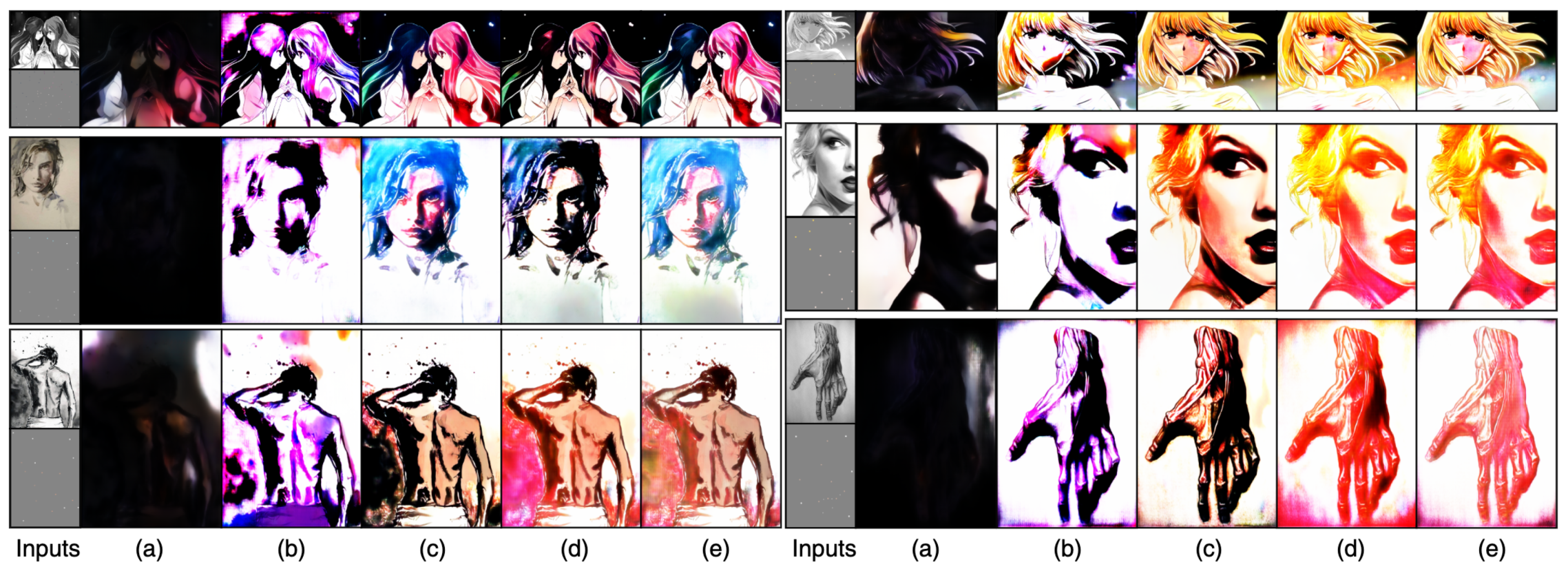
We also tested colorization performance of other styles of image, i.e., grayscale image with various line thickness, texture, and shading. The result is illustrated in Figure 10. In the case of Base model, black was the dominant color and shows a lot of artifacts. Colors in the Pix2Pix model are skewed and also show a lot of artifacts. In the case of proposed model, the model presents a wider color range. Reasons that Base and Pix2Pix cannot properly color the image, unlike the proposed model, is because the distribution of thick lines are not trained and texture present in the image distorts the line distribution.
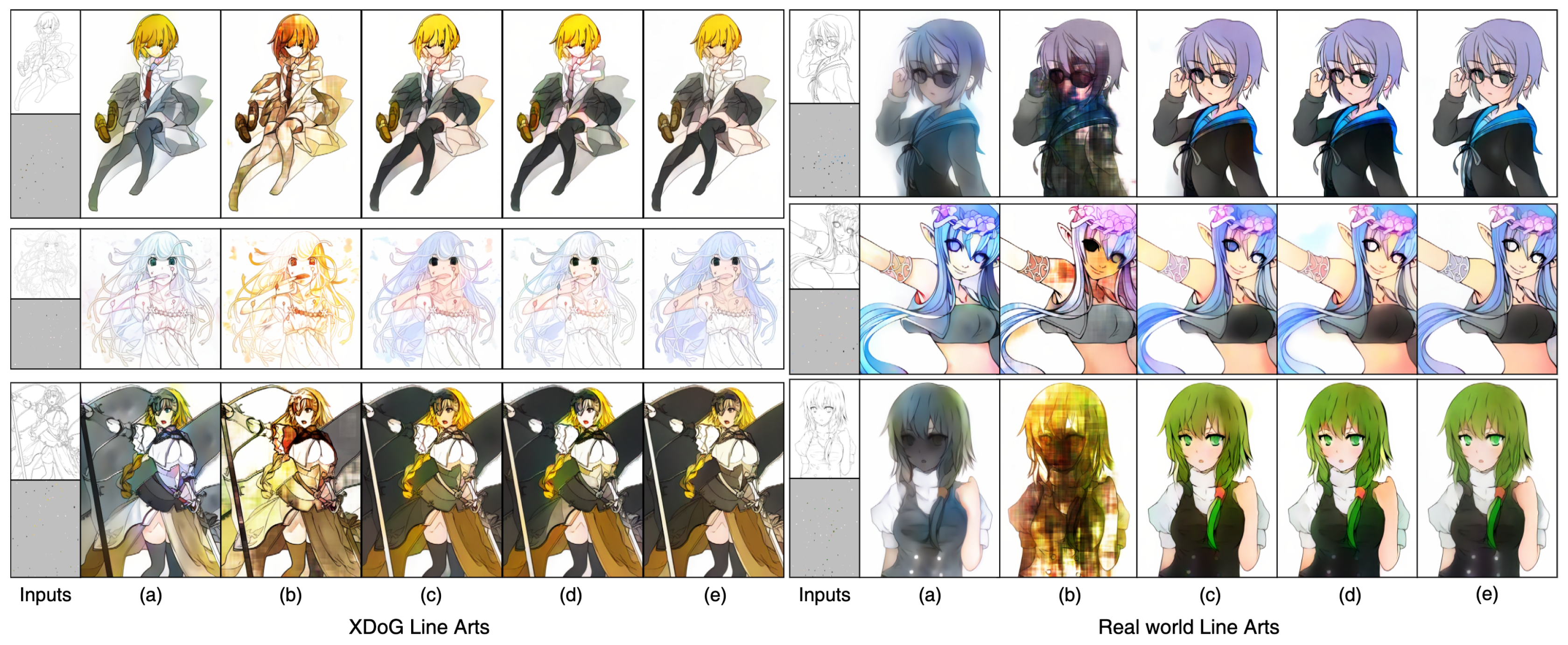
Figure 11 shows the performance of models with 64 randomly chosen color hints leaked from the original color image. To show that our model solves the line overfitting problem, we performed the same experiment on real-world line-arts and lines extracted with XDoG method. Results of Base and Pix2Pix in XDoG line-arts show that they have low accuracy in reflecting input color hints. In the case of Pix2Pix, it shows the checkerboard effect and other artifacts. On the contrary, our model closely follows the original image where hints are given. For example, right collar on the first row of Figure 11e XDoG has colored blue correctly because the hint is given in that region. The left collar is colored with color of hair because the color hint in that region is not given. In the case of real-world line-arts, both Base and Pix2Pix fail to contain the color within the lines. Although Base model tries to color the image with respect to given hints, the colors are spilled and does not follow the given hints. Pix2Pix, on the other hand, consistently shows various artifacts. Consistent with the XDoG case, the colorization of real-world line-arts follows the provided hints. In this case, both of the collars in the first row of Figure 11e real-world are colored with blue which is the color of hints in that region. From Figure 11, we can observe that colorization performance of the proposed model is most stable compared to other models.
4.4. Mean Opinion Score (MOS) Evaluation
The quality of a painting is subjective and varies widely from person. We used Mean Opinion Score (MOS) evaluation to provide objective evaluation of proposed method [2,10]. For evaluation, we asked 118 users to give a score between 1 (bad) and 5 (excellent) based on image quality. A person scores a total of thirty images. There are ten sets of images for three different methods (Base [10], Pix2Pix [2], ours). Each image set is applied to three methods. To have general understanding of the performance of each method, we chose five sets of images in animation style and the other five sets of images in non-animation style. The MOS results are summarized in Table 1 and Figure 12. All users are randomly chosen. MOS of Base [10] and Pix2Pix [2] are 2.56 and 2.75 with 1.30 and 1.34, respectively whereas our method shows MOS of 3.82 and standard deviation of 1.05. Using a level of significance to test the MOS, we can say than our method is superior to the other methods.
4.5. Quantitative Analysis
In order to evaluate the performance of the proposed model, we used the same data set described in Section 4.1 and performed 178 k steps of training on open sourced automatic colorization model used in Ci et al. [10].
To quantitatively measure the difference of models, we used Fréchet Inception Distance (FID) score [31]. FID score measures the similarity of two data sets, and FID is generally known to have high correlation with human judgment of visual quality of a given image. It is often used in evaluating the quality of image generated by GAN. Base image used in FID is generated by Inception model which is trained with ImageNet [27] data set. Target image used in FID is generated by some other model, in our case, two stage generator with histogram equalization and LDM. By applying base and target image on Inception model, we obtain two feature maps. Fréchet distance of normalization of feature map of base and target image gives us the FID score. We used 140K artificial line-arts generated by XDoG and 530 pairs of line-arts and their colorized version of artwork.
Ci et al. [10] and Hati et al. [12] proposed not to use hints while comparing the quality of generated images with FID score because it can not fairly compare the colorization performance of a model. However, FID score is not adequate in measuring colorization performance because it does not take account of color and location information present in the hint. Even if we exploit the hint in measuring FID score, we can not fairly compare the two results unless the location of hints are controlled. Thus, we need to have another performance metric to properly take account of the accurate representation of hint color, locality of color, and color containment within the boundaries of line contours.
In this paper, we propose another performance metric, called Colorization FID (C-FID), specifically designed for comparing the colorization performance. Figure 13 shows the layout of the measurement mechanism. Although, C-FID and FID score are fundamentally the same, the only difference is the use of hint in colorization. C-FID uses segment-based hint pointing method, whereas FID does not use hints. The calculation of the score is the same. We divide an image into seven segments-based on the composition locality present in illustrations. First set of segments are placed in four corners. Let width be w, then we set the dimension of the corner segment as by . We call this region the corner. In between the two corners on the left and and right hand side of the image, there is rectangle segments with dimension of by . This region is called the wing. The rest of the image is called the body. Each corner contain one pixel hint in arbitrary location within the corner. Each wing contains two one pixel hints and the body contains 20 one pixel hints within each wing and body, respectively. Using this constraints, different models can be given a fair comparison because each segment is given a specific number of hint colors within limited space. Then, we measure FID score over the generated images. We call this method of performance measurement as Colorization FID (C-FID).
Table 2 shows the comparison of C-FID scores on different models. Just as FID, the lower the C-FID score is, the better. The result shows that by applying the proposed line loss and histogram equalization, the proposed method achieves lower C-FID than the Base model in all scenarios. There are two interesting observations in the result of C-FID. In the case of real-world line-arts, C-FID score is more than two times larger than that of XDoG line-arts. On the other hand, standard deviation is at least five times lower than that of XDoG line-arts. As we can see from Figure 3, real-world line-art does not contain background texture where as colored version of the line-art is full of texture. As a result, C-FID score becomes high because of the presence of the background texture in the image. The reason behind the low standard deviation is that the training data set of real-world images are about 270 times less than that of XDoG. Thus, we had to crop the original image into 512 × 512 pixel at random locations. Since, we ran an excessively long iteration to learn the given data set, the resulting standard deviation becomes very small.
5. Conclusions
In this paper, we proposed a Line Detection Model (LDM) loss function and histogram equalization for generalization of line distribution. We also proposed a new performance metric called Colorization FID (C-FID) that can provide fair comparison of colorization performance. The experiment results show that the quality of generated image is sensitive to line distribution. The reason for poor quality of generated image is that line distribution of artificially generated line contours is different from real-world line-arts. We compared Base model and the proposed model in four different scenarios. We used XDoG generated line-art and real-world line-arts with and without color hints. The result shows that using histogram equalization and LDM enabled line loss exhibits the best result. The Base model with XDoG generated line-art with and without color hints exhibits C-FID score of 44.70 and 35.83, respectively, whereas the proposed model in the same scenario exhibits 39.77 and 32.16, respectively. C-FID score of real-world line-art with color hint is more dramatic. The Base model exhibits 87.95 and the proposed model exhibits 5.51. From the result, we can conclude that generalization of line distribution leads to better quality of colorized image.
Author Contributions
Conceptualization, Y.L.; data curation, Y.L.; funding acquisition, S.L.; methodology, Y.L.; project administration, S.L.; supervision, S.L.; validation, Y.L. and S.L.; visualization, Y.L.; writing—original draft, Y.L. and S.L.; writing—review and editing, S.L. All authors have read and agreed to the published version of the manuscript.
Funding
This work was supported by the National Research Foundation of Korea (NRF) grant funded by the Korea government (MSIT) (No. 2019R1G1A1100455) and Education and Research Program of AI Convergence Engineering for Industrial Intelligence in Gyeongsangnam-do.
Conflicts of Interest
The authors declare no conflict of interest.
References
- Goodfellow, I.; Pouget-Abadie, J.; Mirza, M.; Xu, B.; Warde-Farley, D.; Ozair, S.; Courville, A.; Bengio, Y. Generative adversarial nets. In Proceedings of the Advances in Neural Information Processing Systems, Montreal, QC, Canada, 8–13 December 2014; pp. 2672–2680. [Google Scholar]
- Isola, P.; Zhu, J.Y.; Zhou, T.; Efros, A.A. Image-to-image translation with conditional adversarial networks. In Proceedings of the IEEE Conference on Computer Vision and Pattern Recognition, Honolulu, HI, USA, 21–26 July 2017; pp. 1125–1134. [Google Scholar]
- Kang, S.; Choo, J.; Chang, J. Consistent comic colorization with pixel-wise background classification. In Proceedings of the NIPS’17 Workshop on Machine Learning for Creativity and Design, Long Beach, CA, USA, 4–9 December 2017. [Google Scholar]
- Furusawa, C.; Hiroshiba, K.; Ogaki, K.; Odagiri, Y. Comicolorization: Semi-automatic manga colorization. In Proceedings of the SIGGRAPH Asia 2017 Technical Briefs, Bangkok, Thailand, 27–30 November 2017; pp. 1–4. [Google Scholar]
- Hensman, P.; Aizawa, K. cGAN-based manga colorization using a single training image. In Proceedings of the 2017 IEEE 14th IAPR International Conference on Document Analysis and Recognition (ICDAR), Kyoto, Japan, 9–15 November 2017; Volume 3, pp. 72–77. [Google Scholar]
- Zhang, L.; Ji, Y.; Lin, X.; Liu, C. Style transfer for anime sketches with enhanced residual u-net and auxiliary classifier gan. In Proceedings of the 2017 IEEE 4th IAPR Asian Conference on Pattern Recognition (ACPR), Nanjing, China, 26–29 November 2017; pp. 506–511. [Google Scholar]
- Sangkloy, P.; Lu, J.; Fang, C.; Yu, F.; Hays, J. Scribbler: Controlling deep image synthesis with sketch and color. In Proceedings of the IEEE Conference on Computer Vision and Pattern Recognition, Honolulu, HI, USA, 21–26 July 2017; pp. 5400–5409. [Google Scholar]
- Liu, Y.; Qin, Z.; Luo, Z.; Wang, H. Auto-painter: Cartoon image generation from sketch by using conditional generative adversarial networks. arXiv 2017, arXiv:1705.01908. [Google Scholar] [CrossRef]
- Frans, K. Outline colorization through tandem adversarial networks. arXiv 2017, arXiv:1704.08834. [Google Scholar]
- Ci, Y.; Ma, X.; Wang, Z.; Li, H.; Luo, Z. User-guided deep anime line art colorization with conditional adversarial networks. In Proceedings of the 26th ACM International Conference on Multimedia, Seoul, Korea, 22–26 October 2018; pp. 1536–1544. [Google Scholar]
- Zhang, L.; Li, C.; Wong, T.T.; Ji, Y.; Liu, C. Two-stage sketch colorization. ACM Trans. Graph. (TOG) 2018, 37, 1–14. [Google Scholar] [CrossRef] [Green Version]
- Hati, Y.; Jouet, G.; Rousseaux, F.; Duhart, C. PaintsTorch: A User-Guided Anime Line Art Colorization Tool with Double Generator Conditional Adversarial Network. In Proceedings of the European Conference on Visual Media Production, London, UK, 17–18 December 2019; pp. 1–10. [Google Scholar]
- Ledig, C.; Theis, L.; Huszár, F.; Caballero, J.; Cunningham, A.; Acosta, A.; Aitken, A.; Tejani, A.; Totz, J.; Wang, Z.; et al. Photo-realistic single image super-resolution using a generative adversarial network. In Proceedings of the IEEE Conference on Computer Vision and Pattern Recognition, Honolulu, HI, USA, 21–26 July 2017; pp. 4681–4690. [Google Scholar]
- Bińkowski, M.; Donahue, J.; Dieleman, S.; Clark, A.; Elsen, E.; Casagrande, N.; Cobo, L.C.; Simonyan, K. High fidelity speech synthesis with adversarial networks. arXiv 2019, arXiv:1909.11646. [Google Scholar]
- Frid-Adar, M.; Klang, E.; Amitai, M.; Goldberger, J.; Greenspan, H. Synthetic data augmentation using GAN for improved liver lesion classification. In Proceedings of the 2018 IEEE 15th international symposium on biomedical imaging (ISBI 2018), Washington, DC, USA, 4–7 April 2018; pp. 289–293. [Google Scholar]
- Radford, A.; Metz, L.; Chintala, S. Unsupervised representation learning with deep convolutional generative adversarial networks. arXiv 2015, arXiv:1511.06434. [Google Scholar]
- Ioffe, S.; Szegedy, C. Batch normalization: Accelerating deep network training by reducing internal covariate shift. arXiv 2015, arXiv:1502.03167. [Google Scholar]
- Dai, B.; Fidler, S.; Urtasun, R.; Lin, D. Towards Diverse and Natural Image Descriptions via a Conditional GAN. In Proceedings of the IEEE International Conference on Computer Vision (ICCV), Venice, Italy, 22–29 October 2017. [Google Scholar]
- Winnemöller, H.; Kyprianidis, J.E.; Olsen, S.C. XDoG: An extended difference-of-Gaussians compendium including advanced image stylization. Comput. Graph. 2012, 36, 740–753. [Google Scholar] [CrossRef] [Green Version]
- Kingma, D.P.; Ba, J. Adam: A method for stochastic optimization. arXiv 2014, arXiv:1412.6980. [Google Scholar]
- Ronneberger, O.; Fischer, P.; Brox, T. U-net: Convolutional networks for biomedical image segmentation. In Proceedings of the International Conference on Medical Image Computing and Computer-Assisted Intervention, Munich, Germany, 5–9 October 2015; Springer: Berlin/Heidelberg, Germany, 2015; pp. 234–241. [Google Scholar]
- Xie, S.; Girshick, R.; Dollar, P.; Tu, Z.; He, K. Aggregated Residual Transformations for Deep Neural Networks. In Proceedings of the IEEE Conference on Computer Vision and Pattern Recognition (CVPR), Honolulu, HI, USA, 21–26 July 2017. [Google Scholar]
- Shi, W.; Caballero, J.; Huszár, F.; Totz, J.; Aitken, A.P.; Bishop, R.; Rueckert, D.; Wang, Z. Real-time single image and video super-resolution using an efficient sub-pixel convolutional neural network. In Proceedings of the IEEE Conference on Computer Vision and Pattern Recognition, Las Vegas, NV, USA, 26 June–1 July 2016; pp. 1874–1883. [Google Scholar]
- Odena, A.; Dumoulin, V.; Olah, C. Deconvolution and checkerboard artifacts. Distill 2016, 1, e3. [Google Scholar] [CrossRef]
- Nah, S.; Hyun Kim, T.; Mu Lee, K. Deep multi-scale convolutional neural network for dynamic scene deblurring. In Proceedings of the IEEE Conference on Computer Vision and Pattern Recognition, Honolulu, HI, USA, 21–26 July 2017; pp. 3883–3891. [Google Scholar]
- Simonyan, K.; Zisserman, A. Very Deep Convolutional Networks for Large-Scale Image Recognition. In Proceedings of the 3rd International Conference on Learning Representations, ICLR 2015, San Diego, CA, USA, 7–9 May 2015; Bengio, Y., Le Cun, Y., Eds.; 2015. [Google Scholar]
- Deng, J.; Dong, W.; Socher, R.; Li, L.; Li, K.; Li, F.-F. ImageNet: A large-scale hierarchical image database. In Proceedings of the 2009 IEEE Conference on Computer Vision and Pattern Recognition, Miami, FL, USA, 20–25 June 2009; pp. 248–255. [Google Scholar]
- Branwen, G. Danbooru2019: A Large-Scale Crowdsourced and Tagged Anime Illustration Dataset. Available online: https://www.gwern.net/Danbooru2019 (accessed on 31 July 2019).
- E-Shuushuu—Kawaii Image Board. 2018. Available online: https://e-shuushuu.net/ (accessed on 19 July 2018).
- Paszke, A.; Gross, S.; Massa, F.; Lerer, A.; Bradbury, J.; Chanan, G.; Killeen, T.; Lin, Z.; Gimelshein, N.; Antiga, L.; et al. PyTorch: An Imperative Style, High-Performance Deep Learning Library. In Advances in Neural Information Processing Systems 32; Wallach, H., Larochelle, H., Beygelzimer, A., d’Alché-Buc, F., Fox, E., Garnett, R., Eds.; Curran Associates, Inc.: Red Hook, NY, USA, 2019; pp. 8024–8035. [Google Scholar]
- Heusel, M.; Ramsauer, H.; Unterthiner, T.; Nessler, B.; Hochreiter, S. GANs trained by a two time-scale update rule converge to a local nash equilibrium. Adv. Neural Inf. Process. Syst. 2017, arXiv:1706.08500. [Google Scholar]
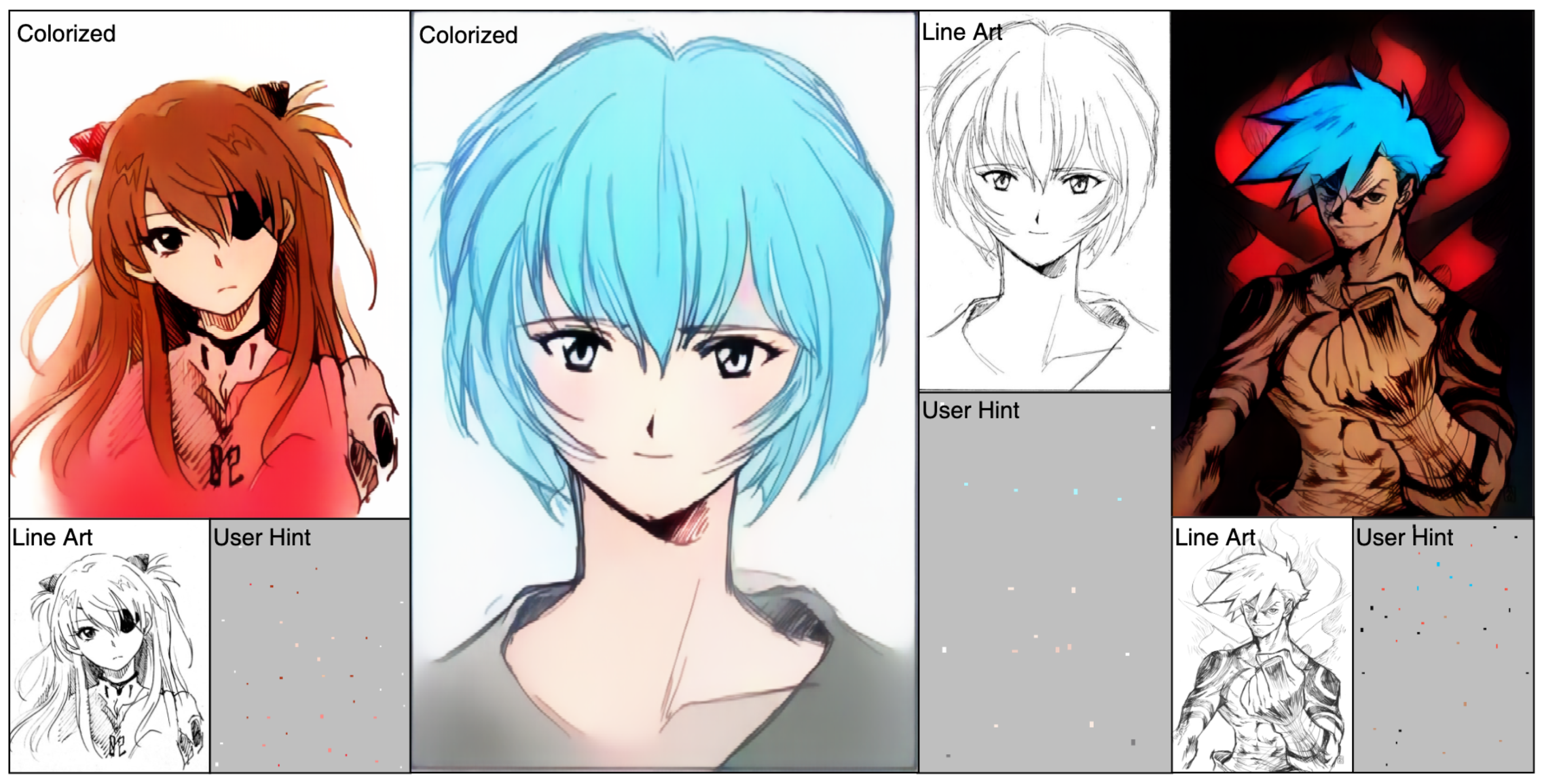
Figure 1.
Proposed method’s real word line-art coloring results.

Figure 2.
Network overview.

Figure 3.
Histogram of line-art (eq: histogram equalization).

Figure 4.
Line-art for Figure 3 (eq: histogram equalization).
Figure 4.
Line-art for Figure 3 (eq: histogram equalization).

Figure 5.
Three pairs of images for pre-processing (Gray has alpha value of 0 in the hint image).

Figure 6.
Line Detection Model (c: output filter number, k: kernel Size, s: stride, For example, c32k3s1 means inter convolution layer output filter number is 32, kernel size is 3, and stride is 1).
Figure 6.
Line Detection Model (c: output filter number, k: kernel Size, s: stride, For example, c32k3s1 means inter convolution layer output filter number is 32, kernel size is 3, and stride is 1).

Figure 7.
Model architecture (c: output filter number, u: output unit number, k: kernel Size, s: stride).
Figure 7.
Model architecture (c: output filter number, u: output unit number, k: kernel Size, s: stride).

Figure 8.
Visual comparison of different models. (a): Base [10], (b): Pix2pix [2], (c): ours (Line Detection Model (LDM) enabled line loss only), (d): ours (histogram equalization only), (e): ours (Both: LDM enabled line loss + histogram equalization).

Figure 9.
Visual comparison of artifacts. (a): Base [10], (b): Pix2pix [2], (c): ours (LDM enabled line loss only), (d): ours (histogram equalization only), (e): ours (Both: LDM enabled line loss + histogram equalization).

Figure 10.
Visual comparison of include grayscale. (a): Base [10], (b): Pix2pix [2], (c): ours (LDM enabled line loss only), (d): ours (histogram equalization only), (e): ours (Both: LDM enabled line loss + histogram equalization).

Figure 11.
Visual comparison of color restoration (a): Base [10], (b): Pix2pix [2], (c): ours (LDM enabled line loss only), (d): ours (histogram equalization only), (e): ours (Both: LDM enabled line loss + histogram equalization).

Figure 12.
Heatmap of Mean Opinion Score (MOS).

Figure 13.
Hint mask for Colorization FID score evaluation.


Table 2.
Quantitative comparison of Colorization FID score. The score measured using total of 145,408 XDoG line-arts and 530 pairs of line-arts and their colorized version of artwork. Lower Colorization FID score is better.
Table 2.
Quantitative comparison of Colorization FID score. The score measured using total of 145,408 XDoG line-arts and 530 pairs of line-arts and their colorized version of artwork. Lower Colorization FID score is better.
| W/O Color Hint | XDoG Line-Arts | Real-World Line-Arts | ||
|---|---|---|---|---|
| Model | FID | STD | FID | STD |
| Base [10] | 44.70 | 2.01 | 109.39 | 0.40 |
| Pix2pix [2] | 41.14 | 1.51 | 117.24 | 0.38 |
| Ours (LDM enabled line loss only) | 43.87 | 1.91 | 99.40 | 0.32 |
| Ours (Histogram equalization Only) | 39.54 | 1.84 | 92.63 | 0.24 |
| Ours | 39.77 | 1.75 | 98.75 | 0.17 |
| With Color Hint | XDoG Line-Arts | Real-World Line-Arts | ||
| Model | C-FID | STD | C-FID | STD |
| Base [10] | 35.83 | 1.81 | 87.95 | 0.36 |
| Pix2pix [2] | 34.21 | 1.12 | 94.14 | 0.31 |
| Ours (LDM enabled line loss only) | 35.51 | 1.74 | 61.83 | 0.26 |
| Ours (Histogram equalization Only) | 33.29 | 1.51 | 60.45 | 0.24 |
| Ours | 32.16 | 1.57 | 57.51 | 0.23 |
Publisher’s Note: MDPI stays neutral with regard to jurisdictional claims in published maps and institutional affiliations. |
© 2020 by the authors. Licensee MDPI, Basel, Switzerland. This article is an open access article distributed under the terms and conditions of the Creative Commons Attribution (CC BY) license (http://creativecommons.org/licenses/by/4.0/).
Share and Cite
MDPI and ACS Style
Lee, Y.; Lee, S. Automatic Colorization of Anime Style Illustrations Using a Two-Stage Generator. Appl. Sci. 2020, 10, 8699. https://0-doi-org.brum.beds.ac.uk/10.3390/app10238699
AMA Style
Lee Y, Lee S. Automatic Colorization of Anime Style Illustrations Using a Two-Stage Generator. Applied Sciences. 2020; 10(23):8699. https://0-doi-org.brum.beds.ac.uk/10.3390/app10238699
Chicago/Turabian StyleLee, Yeongseop, and Seongjin Lee. 2020. "Automatic Colorization of Anime Style Illustrations Using a Two-Stage Generator" Applied Sciences 10, no. 23: 8699. https://0-doi-org.brum.beds.ac.uk/10.3390/app10238699
Note that from the first issue of 2016, this journal uses article numbers instead of page numbers. See further details here.