Development and Validation of Electronic Stability Control System Algorithm Based on Tire Force Observation

Abstract

In view of the higher and higher assembly rate of the electronic stability control system (ESC in short), the control accuracy still needs to be improved. In order to make up for the insufficient accuracy of the tire model in the nonlinear area of the tire, in this paper, an algorithm for the electronic stability control system based on the control of tire force feedforward used in conjunction with tire force sensors is proposed. The algorithm takes into consideration the lateral stability of the tire under extreme conditions affected by the braking force. We use linear optimal control to determine the optimal yaw moment, and obtain the brake wheel cylinder pressure through an algorithm combining feedforward compensation based on measured tire force and feedback correction. The controller structure is divided into two layers, the upper layer is controlled by a linear quadratic regulator (LQR in short) and the lower layer is controlled by PID (Proportional-integral-derivative) and feedforward. After that, verification of the controller’s algorithms using software cosimulation and hardware-in-the-loop (HIL in short) testing in the double lane change (DLC in short) and sine with dwell (SWD in short) conditions. From the test results it can be concluded that the controller based on tire force observation has partially control advantages.

1. Introduction

Electronic stability control (ESC) is an active safety system that controls the braking of the wheels to adjust the body’s posture under extreme conditions. In recent years, the technology of ESC has become more and more mature, and the assembly rate on real vehicles has also become higher. Many researchers have optimized the ESC control strategy through modern control theory and performed simulation verification, and achieved obvious control effects [1]. Daegun Hong et al. of Hanyang University used a braking and wheel slip monitor to propose a target slip rate allocation algorithm for the vehicle stability control system [2]. Sungyeon Ko et al. of Sungkyunwan University proposed a method for a vehicle stability control algorithm for an in-wheel independent drive vehicle using vehicle speed and yaw rate during turning [3]. Li Zhai et al. proposed a new control strategy to improve vehicle stability by using the method of motor drive and regenerative braking torque distribution [4]. Ming Yue et al. introduced a supervisory mechanism for yaw moment control and slip rate adjustment, and proposed a novel control strategy to improve the stability performance of four-wheel independent drive electric vehicles during critical cornering [5]. However, none of the above studies considered that the ESC control strategy is limited by the tire adhesion limit. If the applied braking torque is too large, the lateral stability of the vehicle will be reduced.

The tires are the only component that connects the vehicle to the road. The force of the tires determines the body’s movement posture. Only by making full use of the friction conditions between the tires and the ground can ESC control be more precise [6]. Many scholars have also considered the influence of tire force in the control of the chassis electronic control system. Yue Xiaowei et al. of Tsinghua University used the magic tire formula to develop a vehicle stability control system (VSC in short) based on PID control and differential braking control [7]. Linsheng Jin et al. used the GIM tire model to propose a fuzzy logic controller based on the automotive electronic stability controller system to improve the stability of the vehicle at high speed on low-attached roads [8]. Matteo Corno et al. used the Burkhartd tire model to solve the problem of active lateral dynamics control during braking of four-wheeled vehicles [9]. However, the accuracy of using the tire model to estimate the tire force is limited. Taking the influence of the tire force into consideration, obtaining accurate tire force will help improving the control accuracy of the vehicle chassis electronic control system.

Based on the research results that have been put forward by researchers in the industry [1,2,3,4,5,6,7,8,9], an ESC control algorithm with the tire force sensor to measure the three-component force of the tire is proposed. Based on the consideration of the longitudinal and lateral adhesion limits of the tires, the optimal yaw moment is determined by linear optimal control, and the brake wheel cylinder pressure is obtained by the algorithm combining feedforward compensation and feedback correction. In this paper, Section 2 introduces the composition and working principle of the tire three-component force sensor. Section 3 introduces the control strategy of ESC based on tire force observation. A software cosimulation of the proposed control strategy was carried out in Section 4, using CarSim and Simulink to compare the ESC control algorithm with PID control under double lane change (DLC) and sine with dwell (SWD) conditions. Section 5 uses NI Veristand to perform a hardware-in-the-loop (HIL) comparison test between ESC algorithms using tire force observation and PID control. Section 6 summarizes the full text.

2. Three-Component Force Sensor for Tires

The tire three-component force sensor in spoke form is one of the most common [10]. As shown in Figure 1, the tire force sensor is connected to the rim and rotates with the wheel, and is installed between the rim and the hub. The advantage of the sensor is that the force transmission path of the tire force passes completely through the sensor, and it can detect the tire force accurately. A common spoke-type three-component force sensor consists of the strain gauge, elastomer, encoder, adapter, slip ring and conductor pole etc.

The force measurement principle of the spoke-type three-component force sensor is based on the resistance strain effect, and the resistance value changes with the deformation of the metal conductor under the action of external force. The internal components of the sensor are all installed on the elastic body. The strain gauges for electronic component on the elastomer are attached to the four strain gauge beams between the inner and outer rings of the elastomer, and each beam has eight strain gauges. The wiring form is designed according to the principle of Wheatstone bridge, three sets of output bridges are designed according to different combinations of strain gauges, and then the voltage output in three directions is detected respectively. The output voltages of the three bridges are all weak voltages, and the force values in the three directions of the wheels must be obtained through voltage amplification and the settlement of the coefficient matrix. The sensor of the three-component force rotates with the wheel and the angle changes all the time. Therefore, the encoder needs to be adapted to calculate the angle. When installing the sensor on a wheel, it is also necessary to configure the adapter, slip ring, conductor pole and other accessories. The installation position of the tire three-component force sensor is shown in Figure 2. The strain gauges and the three bridge channels are arranged inside the elastomer, which is shown in the red part in the Figure 2. The elastomer, strain gauges, and the three bridge channels make up the three-component force sensor of the tire.

The tire three-component force sensor is the first generation of smart wheels, which can only detect the force in three directions. In order to have a more comprehensive detection of the mechanical behavior of tires, improvements are made based on the three-component force sensor to design smart-tire six-component force products.

3. Design of Control Strategy

3.1. System Structure

Different from the traditional ESC control strategy, this paper designs a controller based on optimal linear control, and proposes an ESC control strategy based on tire force observation control, in order to be able to use with tire force sensor to improve the control accuracy of the electronic stability control system. First, in the nominal value calculation part, the influence of the maximum lateral force of the tire under extreme conditions by the longitudinal force is considered, and the expected value of the control index is determined according to the road surface information, the vehicle state information, and the measured tire force. After that, based on the nominal and actual values of the control indicators that determine the vehicle’s instability state, if the vehicle is determined to be unstable, the controller will be triggered to work. Next, after the vehicle is determined to be unstable, the upper controller determines the tires to be braked according to the control command. Vehicle state controller outputs target longitudinal force based on desired state. What’s more, the lower controller determines the braking pressure applied to the target wheel based on the target longitudinal force. At last, spoke-type three-component force sensor detects the force of the controlled tire in real time and serves as input to the controller, making the system a closed loop. The controller structure is shown in Figure 3.

3.2. Calculation of Nominal Value

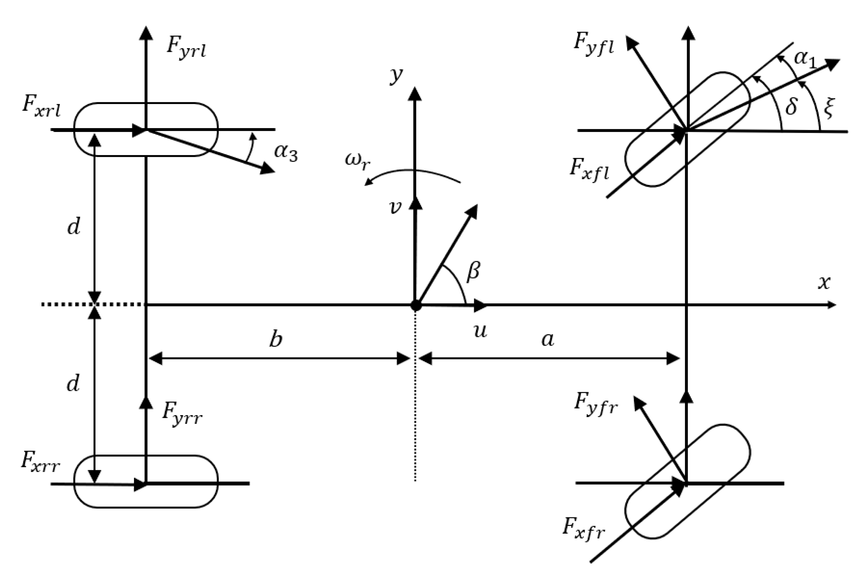
The linear two-degree-of-freedom model is used as the reference model for calculating the nominal value [11,12]. As shown in Figure 4. The differential equation of its motion is shown in Equation (1).

$$\{\begin{array}{c}\left(C_f+C_r\right)\beta +\frac{1}{u}\left(a{C}_f-b{C}_r\right)-C_f\delta =m\left(\dot{v}+u\omega \right)\\ \left(a{C}_f-b{C}_r\right)\beta +\frac{1}{u}\left(a^2{C}_f+b^2{C}_r\right)\omega -a{C}_f\delta =I_z\dot{\omega }\end{array}$$

(1)

Including, $C_f$ is the cornering stiffness for the front axis; $C_r$ is the cornering stiffness for the rear axis; $\beta$ is side slip angle; $u$ is longitudinal speed; $a$ is the distance from the center of mass to the front axis; $b$ is the distance from the center of mass to the rear axis; $\delta$ is the steering angle of front wheels; $m$ is the mass of the vehicle; $\omega$ is the yaw rate; $I_z$ is the moment of inertia of the vehicle around the Z-axis; $\dot{\omega }$ is the yaw acceleration.

Assuming the vehicle is in a steady state, $\dot{v}$ and $\dot{\omega }$ are both equal to zero, meaning ${\omega }_d=G_{\omega }·\delta$, ${\beta }_d=G_{\beta }·\delta$. In simultaneous Equation (1), there are transfer functions characterizing the steady-state yaw rate and the steady-state side slip angle as shown in Equations (2) and (3).

$$G_{\omega }=\frac{u}{L\left(1+k{u}^2\right)}$$

(2)

$$G_{\beta }=\frac{u^2}{L\left(1+k{u}^2\right)}·\left(\frac{b}{u^2}+\frac{ma}{C_{r}L}\right)$$

(3)

where $G_{\omega }$ is the transfer function of the yaw rate; $G_{\beta }$ is the transfer function of the side slip angle; $L$ is the wheelbase; $k$ is the stability factor; ${\omega }_d$ is the expected value of the yaw rate; ${\beta }_d$ is the expected value of the side slip angle.

If the value of the state maximum lateral force is limited according to the pavement friction condition [13,14], the maximum lateral force can be defined as Equation (4) and the centripetal acceleration can be defined as Equation (5). Without regard to the effect of longitudinal forces on the tires, according to the Equations (4) and (5), the expected yaw rate ${\omega }_d$ can be limited as Equation (6). Combining equations ${\omega }_d=G_{\omega }·\delta$ and ${\beta }_d=G_{\beta }·\delta$ can obtain Equation (7), and the limits of the desired side slip angle can be obtained and defined as Equation (8).

$$m\left|a_y\right|\le m\mu g$$

(4)

$$a_y=\dot{v}+u\omega$$

(5)

$$\left|{\omega }_d\right|\le \frac{\mu g}{u}$$

(6)

$${\beta }_d=\frac{G_{\beta }}{G_{\omega }}{\omega }_d$$

(7)

$$\left|{\beta }_d\right|\le \left|\mu g\left(\frac{b}{u^2}+\frac{ma}{k_{2}L}\right)\right|$$

(8)

where $a_y$ is the lateral acceleration of the vehicle; $\mu$ is the coefficient of adhesion between tire and road surface; $g$ is the acceleration due to gravity; $v$ is the lateral speed of vehicle.

The controller in this paper considers the effect of longitudinal force on the lateral force of the tire, and the longitudinal and tangential forces of the tire at the limit of adhesion form a friction circle with a radius less than $\mu$ [15], as shown in Figure 5. With the introduction of tire force feedback, the tire force vector and its longitudinal and lateral components are known, limiting the maximum value of the state according to the friction circle. Expressed in Equation (9).

$$F_{ymax}={{\displaystyle \sum }}_{i=1}^2\left(\sqrt{{\left(F_{zi}{\mu }_i\right)}^2-F_{xi}^2}·cos\delta +F_{xi}·sin\delta \right)+{{\displaystyle \sum }}_{i=3}^4\sqrt{{\left(F_{zi}{\mu }_i\right)}^2-F_{xi}^2}$$

(9)

In the Equation (9), $F_{ymax}$ is the maximum lateral force of vehicle; $F_{zi}$ is the vertical force of tire; $F_x$ is the longitudinal force of tire; in addition, $i$ = 1, 2, 3, 4, They represent left front, right front, left rear and right rear wheels respectively.

Replacing Equation (4) $m\left|a_y\right|\le m\mu g$ with $m\left|a_y\right|\le F_{ymax}$ obtains a constraint on the value of the maximum lateral force for the desired state based on real-time tire force observations.

3.3. Judgment of Vehicle Stability

Under the extreme conditions, using formula (10) and formula (11) to determine whether the vehicle is unstable.

Under extreme conditions, use Equations (10) and (11) to determine whether the vehicle is unstable. Equation (10) is the judgment condition for yaw rate, Equation (11) is the judgment condition for the side slip angle. When the vehicle state satisfies either one of (10), (11), it is in vehicle instability [16].

$$\left|\Delta \omega \right|\le C{\omega }_{NO}$$

(10)

$$\left|B_1\dot{\beta }+\beta \right|\le \mu B_2$$

(11)

Among them, $\Delta \omega$ is the difference between yaw rate and nominal yaw rate; ${\omega }_{NO}$ is the nominal yaw rate. $C$, $B_1$, $B_2$ are stability coefficients. According to experiences $C$ = 0.165, $B_1$ = 0.4, $B_2$ = 0.12.

3.4. The Selection of Control Wheel

Using the same side two-wheel control, adopting the positive and negative yaw rate deviation and the front wheel steering to determine whether to control the left wheel or the right wheel. Through comprehensive analysis, when the Equation (12) is satisfied, the left wheel is controlled to satisfy the Equation (13) when controlling the right wheel.

$$\Delta \omega =\omega -{\omega }_{NO}<0$$

(12)

$$\Delta \omega =\omega -{\omega }_{NO}>0$$

(13)

To prevent the brake command from switching back and forth between the wheels on both sides, the following explains the logic when the left wheel is under braking control. When the left wheel is under brake control, $\Delta \omega <0$, switching from left wheel braking control to right wheel braking control is subject to Equation (14) and Equation (15). The switching logic of the left and right sides wheel braking control is shown in Figure 6.

$$\Delta \omega >D$$

(14)

$$\Delta \omega /\left|{\omega }_{NO}\right|>P$$

(15)

Among them, $D$ and $P$ are the threshold value set. $D$ and $P$ represent the absolute error and the relative error of the yaw rate respectively, the two together constitute the switching criterion for the control of left and right-side wheel. When the values of $D$ and $P$ are small, the control accuracy is high, and the overshoot of yaw rate is small, but the wheel control on both sides is switched frequently, and the yaw rate jitter is obvious. When the values of $D$ and $P$ are large, the control accuracy is low and the overshoot of yaw rate is large, but the wheel control on both sides is not switched frequently, and the yaw rate hardly shakes. In practical applications, the balance between control accuracy and jitter should be weighed and the switching threshold should be set reasonably.

3.5. Upper Control Strategy

The longitudinal force of the tire is directly changed by braking to control the stability of the vehicle. According to the left and right sides control, different differential equations are listed: the resultant lateral force is shown in Equation (16), and the total moment of inertia in the vertical direction is shown in Equation (17).

$$m\left(\dot{v}+um\right)={{\displaystyle \sum }}^{ }{F}_y$$

(16)

$$I_z\dot{\omega }={{\displaystyle \sum }}^{ }{M}_z$$

(17)

where, ${{\displaystyle \sum }}^{ }{F}_y$ is the resultant lateral force of vehicle; ${{\displaystyle \sum }}^{ }{M}_z$ is the total moment about the vertical direction.

From the equation of equilibrium for yaw motion, as shown in Equation (18), left wheel control can be derived as shown in Equations (19) and (20).

$$\begin{array}{l}{I}_z·\dot{\omega }=\left[\left(F_{xfl}+F_{xfr}\right)sin\delta +\left(F_{yfl}+F_{yfr}\right)cos\delta \right]·a\\ +\left[\left(F_{xfr}-F_{xfl}\right)cos\delta +\left(F_{yfl}-F_{yfr}\right)sin\delta \right]·d+\left(F_{xrr}-F_{xrl}\right)·d\\ -\left(F_{yrl}-F_{yrr}\right)·d\end{array}$$

(18)

$$\dot{\beta }=-\omega +\frac{{{\displaystyle \sum }}^{ }{F}_y}{mu}$$

(19)

$$\dot{\omega }=\frac{z_1}{I_z}+\frac{F_{xrl}d+F_{xfl}\left(cos\delta ·d-sin\delta ·a\right)}{I_z}$$

(20)

Inside, $F_{xfl}$ is the longitudinal force on the left front wheel; $F_{xrl}$ is the longitudinal force on the left rear wheel; $z_1$ is the measurable distractors moment; $z_1=-\left[F_{xfr}sin\delta +\left(F_{yfl}+F_{yfr}\right)cos\delta \right]·a-\left[F_{xfr}cos\delta +\left(F_{yfl}-F_{yfr}\right)sin\delta \right]d-F_{xrr}·d+\left(F_{yrl}-F_{yrr}\right)·b$.

Inside, $F_{xrl}$ is the longitudinal force on the right front wheel; $F_{xrr}$ is the longitudinal force on the right rear wheel; $F_{yfl}$ is the lateral force on the left front wheel; $F_{yfr}$ is the lateral force on the right front wheel; $F_{yrl}$ is the lateral force on the left rear wheel; $F_{yrr}$ is the lateral force on the right rear wheel; $d$ is the half of wheelbase.

Right-hand wheel control is as shown in Equations (21) and (22):

$$\dot{\beta }=-\omega +\frac{{{\displaystyle \sum }}^{ }{F}_y}{mu}$$

(21)

$$\dot{\omega }=\frac{z_2}{I_z}+\frac{-F_{xrr}d-F_{xrl}\left(cos\delta ·d+sin\delta ·a\right)}{I_z}$$

(22)

Inside, is the measurable distractors moment, and $z_2=-\left[F_{xfl}sin\delta +\left(F_{yfl}+F_{yfr}\right)cos\delta \right]·a+\left[F_{xfl}-\left(F_{yfl}-F_{yfr}\right)sin\delta \right]·d+F_{xrl}·d+\left(F_{yrl}-F_{yrr}\right)·b$.

To facilitate the design of the controller, the left- and right-side controls are written as a unified expression. The equation of state is shown in Equations (23) and (24) as follows.

$$\dot{\beta }=-\omega +s$$

(23)

$$\dot{\omega }=z+U$$

(24)

where $s$ is the interference term of side slip angle, and $s=\frac{{{\displaystyle \sum }}^{ }{F}_y}{mu}$; $z$ is the measurable interference of the yaw rate, and the expression is shown in Equation (25); $U$ is the virtual control unit, shown in Equation (26).

$$z=\{\begin{array}{c}\frac{z_1}{I_z} ; control of left side \\ \frac{z_2}{I_z} ; control of right side \end{array}$$

(25)

$$U=\{\begin{array}{c}\frac{F_{xrl}d+F_{xfl}\left(cos\delta ·d-sin\delta ·a\right)}{I_z};control of left side \\ \frac{-F_{xrr}d-F_{xfr}\left(cos\delta ·d-sin\delta ·a\right)}{I_z};control of right side\end{array}$$

(26)

The equation of state is formulated into the error form as shown in Equations (27) and (28).

$$\dot{e_1}=\dot{{\beta }_d}-\dot{\beta }=\dot{{\beta }_d}-\left(-\omega +s\right)=-\left({\omega }_d-\omega \right)+\left({\omega }_d+\dot{{\beta }_d}-s\right)=-e_2+s^{\prime }$$

(27)

$$\dot{e_2}=\dot{{\omega }_d}-\dot{\omega }=\dot{{\omega }_d}-z-U=U^{\prime }$$

(28)

where $e_1$ is the error of the side slip angle; $e_2$ is the error of the yaw rate. Inside, $s^{\prime }=\left({\omega }_d+\dot{{\beta }_d}-s\right)$; $U^{\prime }=\dot{{\omega }_d}-z-U$.

Presented in matrix form as in formula (29).

$$\left[\begin{array}{c}\dot{e_1}\\ \dot{e_2}\end{array}\right]=A\left[\begin{array}{c}{e}_1\\ e_2\end{array}\right]+B{U}^{\prime }+\left[\begin{array}{c}1\\ 0\end{array}\right]s^{\prime }$$

(29)

Inside, $A=\left[\begin{array}{cc}0& -1\\ 0& 0\end{array}\right]$; $B=\left[\begin{array}{c}0\\ 1\end{array}\right]$.

To determine the controllability of the system, $Rank\left(B,AB\right)=2$, when the matrix satisfies the full rank.

In this paper, the feedback gain matrix for closed-loop control is designed by the LQR control algorithm to define the performance index function as shown in Equation (30).

$$J=\frac{1}{2}{{\displaystyle \int }}^{ }{e}^{T}Qe+{U^{\prime }}^{T}R{U}^{\prime }$$

(30)

where $Q$ is the error weight matrix; $R$ is the input weighting factor; the Riccati equation can be obtained as shown in Equation (31).

$$-PA-A^{T}P+PB{R}^{-1}{B}^{T}P-Q=0$$

(31)

Solving the algebraic Riccati equation, we can get the $P$, then the feedback gain matrix can be equal to $K$, $K=-R^{-1}{B}^{T}Px\left(t\right)$, and then $U^{\prime }=\dot{{\omega }_d}-z-\mathrm{U}=-k_1{e}_1-k_2{e}_2$, thus $U=k_1{e}_1+k_2{e}_2+\dot{{\omega }_d}-z$, $K=\left[\begin{array}{cc}{k}_1& k_2\end{array}\right]$.

Therefore, the brake for the left wheel is as in Equation (32):

$$U=k_1{e}_1+k_2{e}_2+\dot{{\omega }_d}-z=\frac{F_{xrl}d+F_{xfl}\left(cos\delta ·d-sin\delta ·a\right)}{I_z}$$

(32)

Then we get the Equation (33):

$$F_{xrl}d+F_{xfl}\left(cos\delta ·d-sin\delta ·a\right)=I_z\left(k_1{e}_1+k_2{e}_2+\dot{{\omega }_d}\right)-z_1$$

(33)

the brake for the right wheel is as in Equation (34):

$$U=k_1{e}_1+k_2{e}_2+\dot{{\omega }_d}-z=\frac{-F_{xrr}d-F_{xfr}\left(cos\delta ·d+sin\delta ·a\right)}{I_z}$$

(34)

After that, we can get the Equation (35):

$$F_{xrr}d+F_{xfr}\left(cos\delta ·d+sin\delta ·a\right)=-I_z\left(k_1{e}_1+k_2{e}_2+\dot{{\omega }_d}\right)+z_2$$

(35)

Due to the small longitudinal acceleration, the front and rear axle-load transfer is small. The front and rear longitudinal force is distributed according to the static axle load: $\frac{F_{Xf}}{F_{xr}}=\frac{b}{a}$.

The constraint of maximum longitudinal force is based on the current friction circle to constrain the maximum longitudinal force, which is defined as Equation (36):

$$F_{xi}\le \sqrt{{\left(F_{zi}\mu \right)}^2-F_{yi}^2}$$

(36)

In addition, due to the existence of driving force, the calculated target longitudinal force can be a negative value, if its absolute value is not greater than the current driving force of the tire.

3.6. Lower Control Strategy

The final input to the vehicle due to the controller for tire force observation is the brake cylinder pressure, it is therefore necessary to convert the longitudinal force of the target tire into the target braking pressure. The tire force controller adopts feedforward and feedback control strategies as shown in Equations (37) and (38).

$$P_f=\frac{\left(F_{xb\_ref}+F_t\right)r}{C_b}$$

(37)

$$P_b=K_p\left(F_{xb\_ref}-F_{xb}\right)$$

(38)

where $P_f$ is the feed-forward brake-pressure; $F_{xb\_ref}$ is the target brake pressure; $F_t$ is the driving force; $r$ is the tire rolling radius; $C_b$ is the brake efficiency factor; $P_b$ is the feedback brake pressure; $K_p$ is the feedback gain; $F_{xb}$ is the actual brake-pressure.

Feedforward is the corresponding relationship between braking force and braking pressure under completely ideal conditions, which can improve the response speed of the system; feedback is used to reduce errors and improve control accuracy.

4. Software Cosimulation

The controller in this paper was simulated and analyzed by software in a Simulink environment and the vehicle dynamics model was in CarSim, which uses a nonlinear tire model. The ISO3888-2 Double Lane Change avoidance condition and FMVSS 126 Sine with Dwell were studied and analyzed in comparison with the conventional PID control algorithm in ESC, which the PID controller is not based on tire force sensor.

4.1. Double Lane Change Condition

In the Double Lane Change condition, the vehicles were set up for simulation testing at different speeds on different adhesion coefficients of pavement. Two pavements with adhesion coefficients of 0.5 and 0.8 were selected to represent the low and high attached pavement respectively, and the vehicle speed was selected to be 80 km/h, 100 km/h and 120 km/h, the three speed limits commonly applied to vehicles.

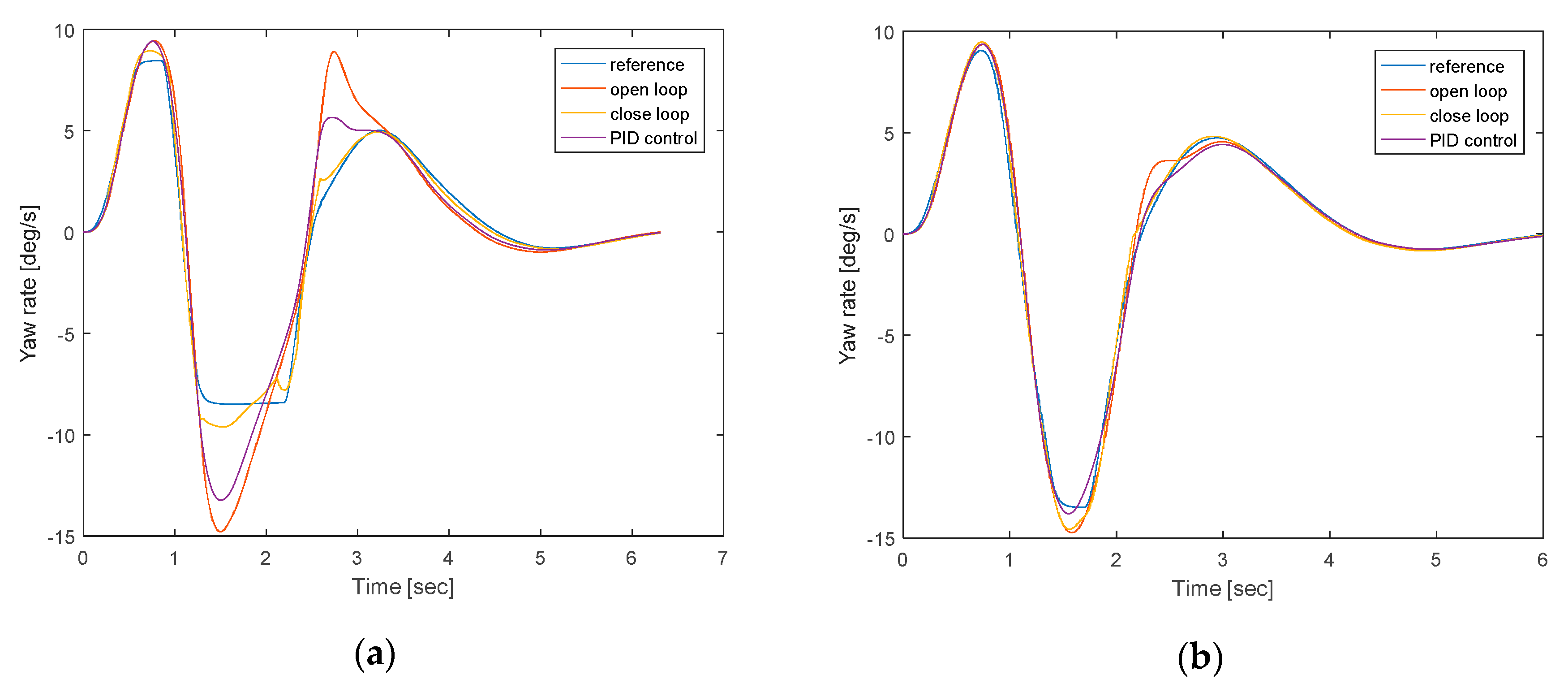
In the Figure 7, Figure 8 and Figure 9, the reference represents the nominal yaw rate calculate by the controller proposed in this article; the open loop represents the yaw rate without the controller, but still keeps the driver model; the closed loop represents the yaw rate with the controller in this pa per; and the PID control represents the yaw rate with traditional PID control, for which the PID controller is not based on a tire force sensor.

According to the simulation results shown in Figure 7, Figure 8 and Figure 9, it can be concluded that the control effect of the ESC controller with tire force observation-based control is more pronounced on low-adhesion surfaces. The better the follow-through of the nominal yaw rate for vehicles controlled with this controller, the more pronounced this phenomenon will be with increasing speed. On high adhesion coefficient pavements, the difference between the two control methods is not obvious, and there is a small error in the simulation results.

4.2. Sine with Dwell Condition

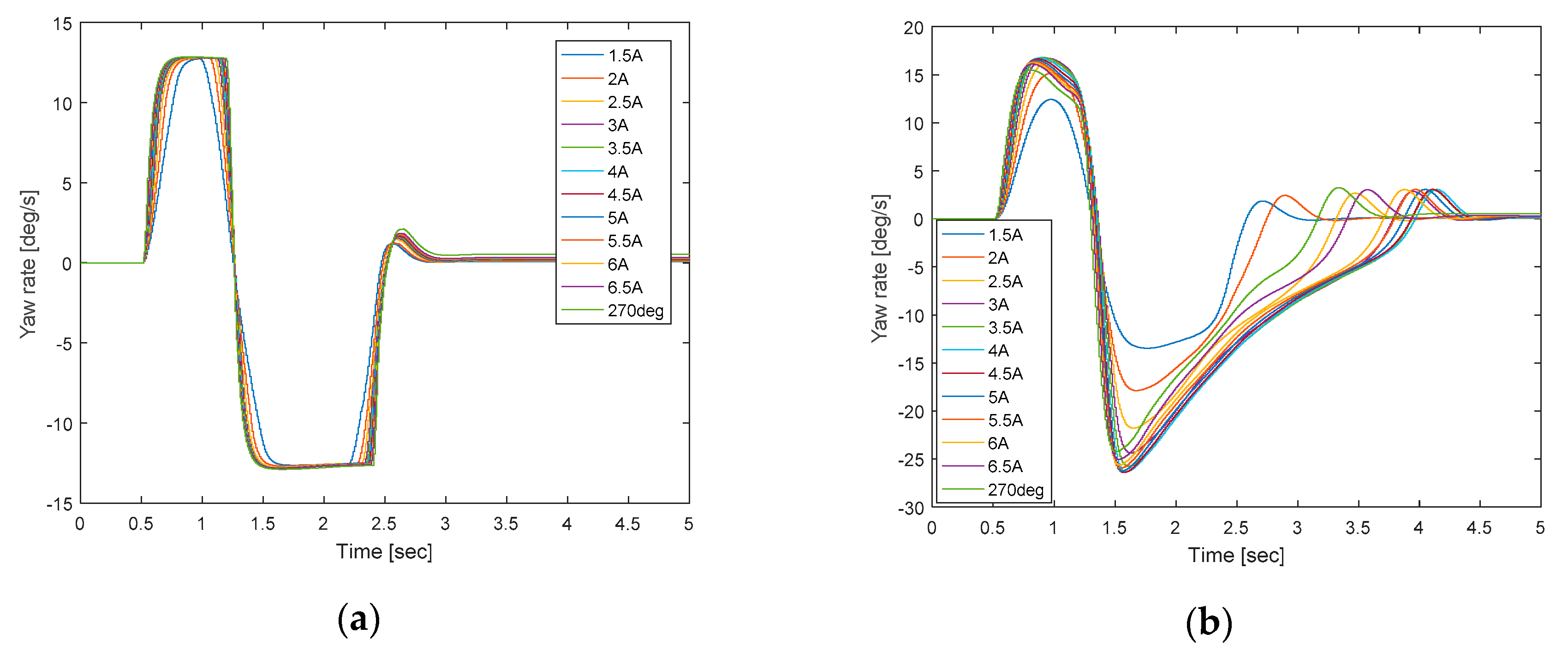
The sine with dwell (SWD) simulation test follows the standard FMVSS 126 requirements to set up the simulation conditions. According to the simulation of the vehicle model used to obtain A = 13 deg. At a speed of 80 km/h on the road surface adhesion coefficient of 0.5 and 0.8 on the test, each condition was drawn to 1.5 A, 2 A, 2.5 A, …, 6.5 A and 270 deg as the maximum values of the yaw rate for the sinusoidal steer angle.

Based on Figure 10 and Figure 11, it can be concluded that the vehicle model without the controller already produces severe skidding under the simulated conditions at both low and high road adhesion coefficients. In the case of low-road-adhesion coefficient, the situation of following the nominal value and jitter of the ESC controller based on tire force observation is better than those of the traditional PID control. In the case of a high road adhesion coefficient, no significant difference in the following of nominal yaw rate between ESC controller based on tire force observation and conventional PID control, and there are small fluctuations in the yaw rate for both control methods.

5. Hardware-in-the-Loop Test

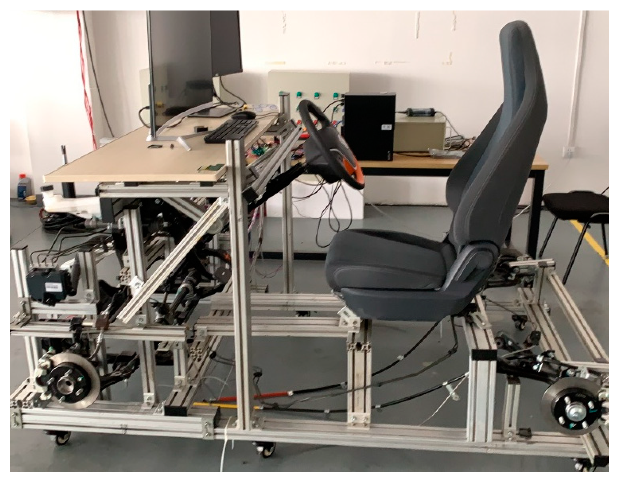
The HIL test of this controller was done in an NI Veristand real-time simulation system, the upper computer used the CarSim vehicle model, and the control strategy was built in the Simulink environment. The HIL frame contained the ESC system, braking circuit, wheel cylinder pressure sensor, upper computer, lower computer, and the corresponding function boards, shown in Figure 12. An HIL comparison test was performed under the same conditions as in Section 4.

5.1. Double Lane Change Condition

In this part of the HIL test, the settings of vehicle speed and coefficient of pavement adhesion were consistent with the software cosimulation, using the common high speeds of 80 km/h and 100 km/h, and the pavement adhesion coefficient was set at 0.5 and 0.8.

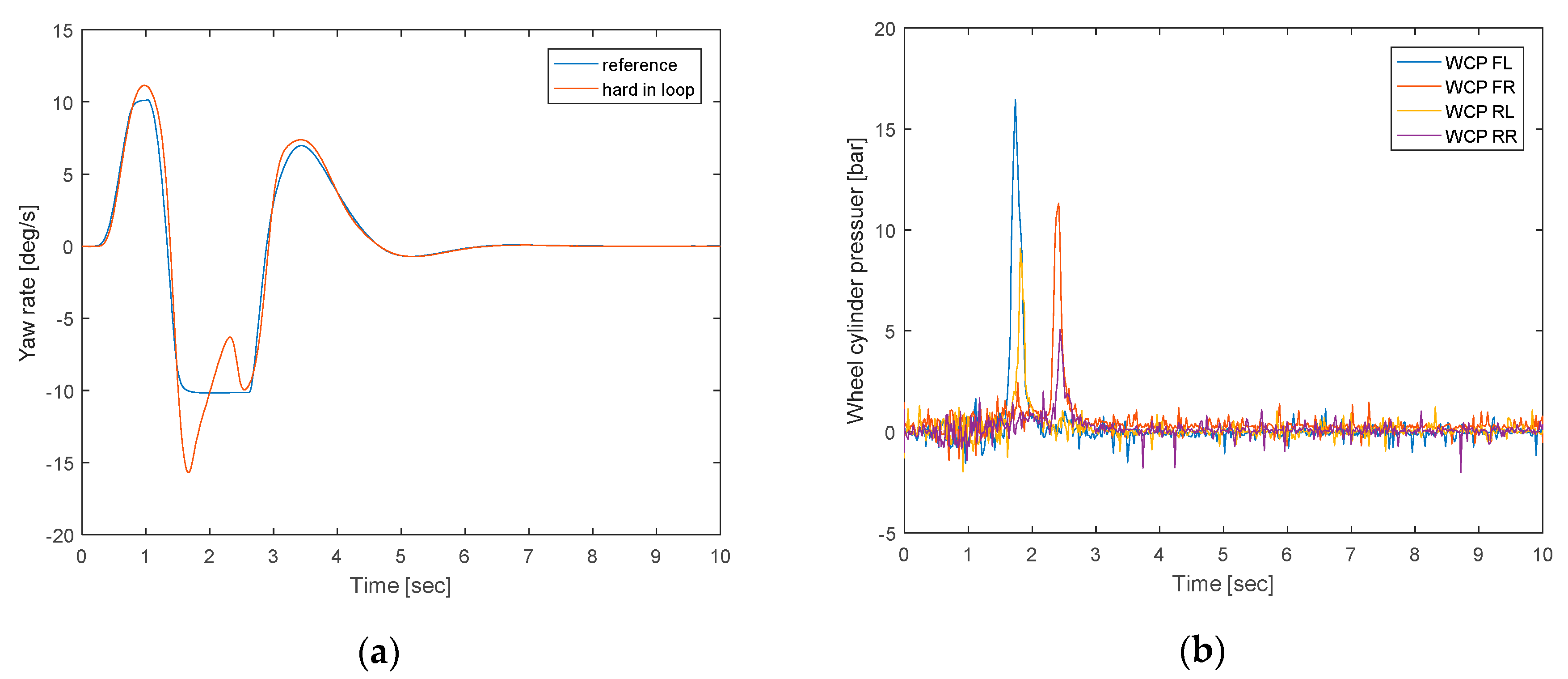
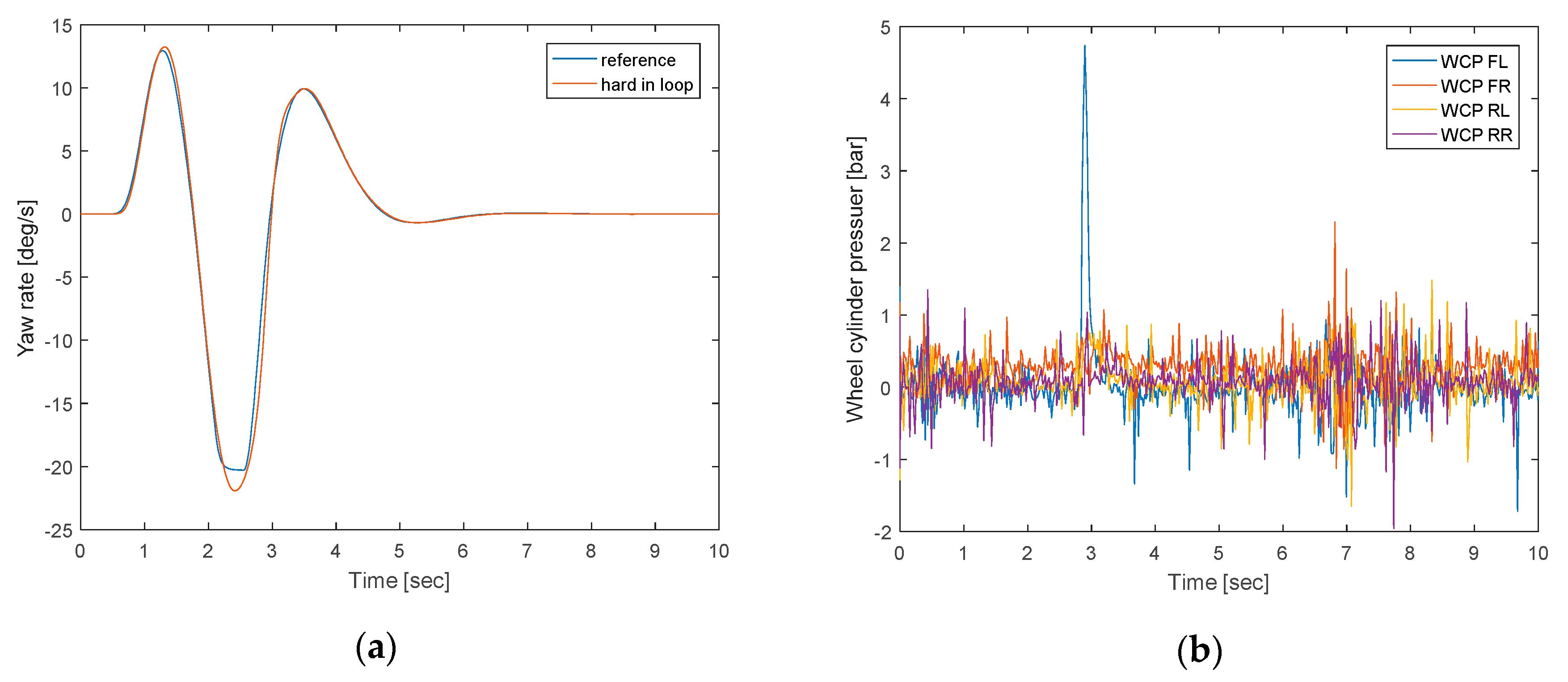
In the hardware-in-the-loop test under the double lane change condition, the vehicle model based on tire force observation in the low pavement adhesion coefficient condition followed the nominal yaw rate better than the traditional PID control, and the vehicle model based on tire force observation at the peak of the yaw rate curve had a clear advantage over the traditional PID control. However, when the value of the yaw rate was close to the largest negative value, the yaw rate of the vehicle models controlled by the two controllers had a certain fluctuation. Comparing the test time on the abscissa of a and b in Figure 13, Figure 14, Figure 15, Figure 16, Figure 17, Figure 18, Figure 19 and Figure 20, it can be seen that the response time of the actuator brake pressure value slightly lagged behind the time at which the yaw rate curve separated greatly. Therefore, the high-frequency braking signal caused the actual response pressure of the brake wheel cylinder to be insufficient. Thus, it affected the actuator control of the vehicle model and made the yaw rate following worse.

In high road adhesion conditions, the actuators controlled by the two controllers hardly trigger work. As far as the yaw rate follows, the controller based on tire force observation has obvious advantages. The test conditions of high and low road adhesion coefficients at a speed of 120 km/h are almost the same as those at a speed of 100 km/h.

5.2. Sine with Dwell Condition

The setting of vehicle speed and road adhesion coefficient in the sine with dwell condition in the loop test is consistent with the software co-simulation. The vehicle speed is set to 80 km/h, the road adhesion coefficient is 0.5 and 0.8, and the peak steering angle is 1.5 A, 2 A, 2.5 A, …, 6.5 A and 270 deg respectively.

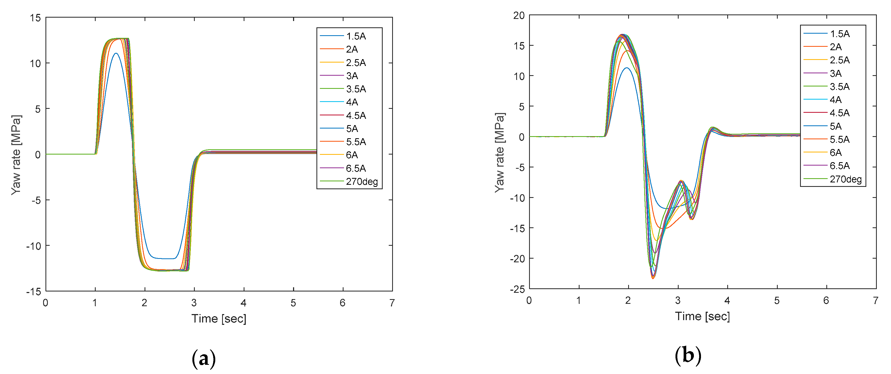
Compared with the software co-simulation, as shown in Figure 21, Figure 22, Figure 23, Figure 24, Figure 25 and Figure 26, firstly, the overshoot caused by the fluctuation of the yaw rate during the steering hysteresis phase of the test of the controller designed in this paper is smaller than that of the vehicle model with PID controller under the low adhesion coefficient condition. Secondly, the fluctuation of the yaw rate for the controller based on tire force observation during the steering hysteresis phase is larger for the vehicle model with PID control. Thirdly, at high pavement adhesion coefficients, the yaw rate response of the vehicle model with both controllers is improved at lower pavement adhesion coefficients, and the nominal yaw rate response of the vehicle model with the PID controller is also improved at lower pavement adhesion coefficients, both controller-controlled vehicle models have improved yaw rate response to low pavement adhesion coefficients, and also improved the follow-through of nominal yaw rate for low pavement adhesion coefficients conditions. Among them, the improvement in the yaw rate response of the vehicle model based on tire force observations is more pronounced.

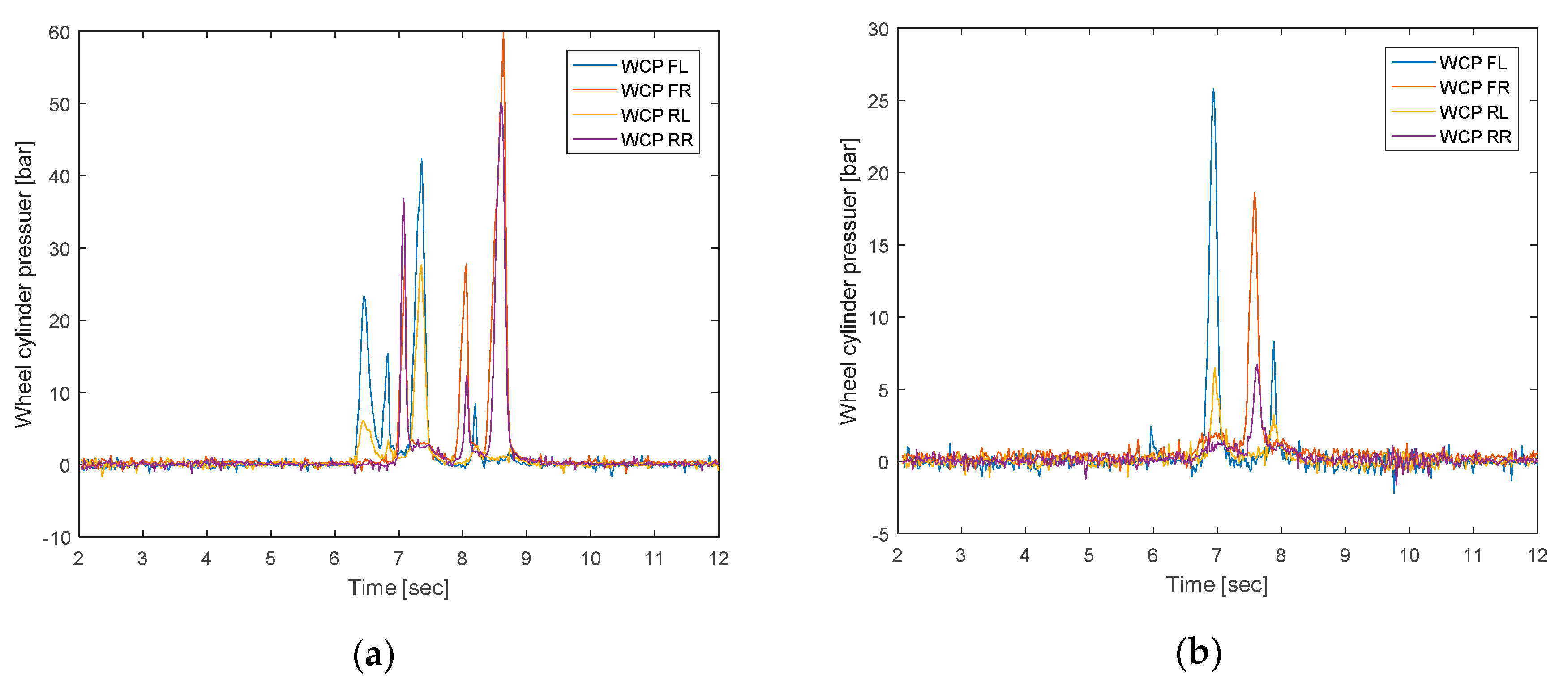
According to the images of brake cylinder pressure shown in Figure 23 and Figure 26, it can be concluded that there is a certain discrepancy between the yaw rate of actual value and nominal value after the controller control as well as a small range of fluctuation, this is caused by a delay in the brake hydraulic circuit for a certain period of time, insufficient response to high frequency braking signals, and inconsistent response of the front and rear wheels to braking pressure.

6. Discussion

In the software cosimulation, different vehicle speeds and different road adhesion coefficients were tested. As the vehicle speed increases, the ESC control algorithm based on the tire force sensor shows better stability. The PID-controlled ESC control algorithm will have a significant overshoot and the nominal yaw rate value will not follow tightly as the vehicle speed increases. The difference between the different ESC control algorithms on the road with low adhesion coefficient is more obvious. Generally speaking, the ESC controller based on tire force control follows the situation of the nominal yaw rate better than the traditional PID controller (without the tire force sensor), the difference between the two is not obvious on the road with high adhesion coefficient.

In the hardware-in-the-loop test, in addition to obtaining the same conclusions as in the software cosimulation, it can also be concluded from the wheel cylinder pressure diagram in the sine with dwell condition that the conventional PID controller sends signals to the actuator more frequently than the ESC controller based on the tire force sensor, which indicates that the ESC control algorithm based on the tire force sensor can effectively improve the efficiency of ESC control of the vehicle, improve the control accuracy, and reduce the number of false triggers. However, this conclusion still needs to be further tested and verified.

Compared with the traditional PID-controlled controller, the ESC controller based on tire force observation in this paper shows some advantages in the case of a low road adhesion coefficient and improves the following situation of the nominal value of yaw rate. This proves that the use of the tire force collected by the tire force sensor as the input of the ESC controller can compensate for the inaccurate expression of the tire model under extreme operating conditions and nonlinear conditions, thus proving that the use of a controller based on tire force observation can be a new idea to improve the control accuracy of the chassis electronic control system.

There are still some limitations to this paper. Firstly, under extreme conditions, there is a large difference in the follow-through of the actual value to the nominal value of the side slip angle, but the vehicle is still in a stable state that does not require ESC access control. Therefore, this article does not carry out the test results of the side slip angle analysis. Secondly, another question is mostly focused on the actuator response in the hardware-in-the-loop test. The actuator response accuracy and rate will have a large impact on the control effect of the ESC controller; therefore, future work will focus on the controller algorithm to consider the inherent problems of the actuator and improve the speed of solenoid valve boosting in ESC.

References

- Van Zanten, A.; Erhardt, R.; Landesfeind, K.; Pfaff, G. VDC Systems Development and Perspective. SAE Trans. 1998, 107, 424–444. [Google Scholar]
- Hong, D.; Hwang, I.; Yoon, P.; Huh, K. Development of a Vehicle Stability Control System Using Brake-by-Wire Actuators. J. Dyn. Syst. Meas. Control 2008, 130, 141–148. [Google Scholar] [CrossRef]
- Ko, S.; Ko, J.; Lee, S.; Cheon, J.; Kim, H. Development of a vehicle stability control algorithm using velocity and yaw rate for an in-wheel drive vehicle. In Proceedings of the 2012 IEEE Vehicle Power and Propulsion Conference, Seoul, Korea, 9–12 October 2012. [Google Scholar]
- Zhai, L.; Sun, T.; Wang, J. Electronic Stability Control Based on Motor Driving and Braking Torque Distribution for a Four In-Wheel Motor Drive Electric Vehicle. IEEE Trans. Veh. Technol. 2016, 65, 4726–4739. [Google Scholar] [CrossRef]
- Yue, M.; Yang, L.; Sun, X.; Xia, W. Stability Control for FWID-EVs with Supervision Mechanism in Critical Cornering Situations. IEEE Trans. Veh. Technol. 2018, 67. [Google Scholar] [CrossRef]
- Audisio, G.; Cheli, F.; Melzi, S.; Velardocchia, M. Cybertm tyre for vehicle active safety. Proc. XIX AIMETA 2009, 14–17. [Google Scholar]
- Yue, X.; Zhang, J.; Lv, C.; Gao, J.; Kong, D. Computational simulation on VSC based on PID coordinated control algorithm and differential brake. In Proceedings of the IEEE Vehicle Power & Propulsion Conference, Beijing, China, 15–18 October 2013. [Google Scholar]
- Jin, L.; Xie, X.; Shen, C.; Wang, F.; Wang, F.; Ji, S.; Guan, X.; Xu, J. Study on electronic stability program control strategy based on the fuzzy logical and genetic optimization method. Adv. Mech. Eng. 2017, 9, 168781401769935. [Google Scholar] [CrossRef] [Green Version]
- Corno, M.; Tanelli, M.; Boniolo, I.; Savaresi, S. Advanced Yaw Control of Four-wheeled Vehicles via Rear Active Differential Braking. In Proceedings of the 48th IEEE Conference on the Decision and Control 2009 Held Jointly with the 2009 28th Chinese Control Conference (CDC/CCC 2009), Shanghai, China, 16–18 December 2009. [Google Scholar]
- Gobbi, M.; Mastinu, G.; Previati, G.; Pennati, M. 6-Axis Measuring Wheels for Trucks or Heavy Vehicles. SAE Int. J. Commer. Veh. 2014, 7, 141–149. [Google Scholar] [CrossRef]
- Tseng, H.E.; Ashrafi, B.; Madau, D.; Brown, T.A.; Recker, D. The development of vehicle stability control at Ford. IEEE/ASME Trans. Mechatron. 1999, 4, 223–234. [Google Scholar] [CrossRef]
- Weiss, Y.; Allerhand, L.I.; Arogeti, S. Yaw stability control for a rear double-driven electric vehicle using LPV-H∞ methods. Sci. China Inf. Sci. 2018, 61, 70206. [Google Scholar] [CrossRef] [Green Version]
- Van Zanten, A. Evolution of electronic control systems for improving the vehicle dynamic behavior. In Proceedings of the 6th International Symposium on Advanced Vehicle Control, Hiroshima, Japan, 9–12 September 2002. [Google Scholar]
- He, X.; Yang, K.; Ji, X.; Liu, Y.; Deng, W. Research on Vehicle Stability Control Strategy Based on Integrated-Electro-Hydraulic Brake System. In Proceedings of the WCX 17: SAE World Congress Experience, Detroit, MI, USA, 4–6 April 2017. [Google Scholar]
- Guo, K.; Ding, H. The Effect of Yaw Moment through Differential Braking under Tire Adhesion Limit. SAE-China 2002, 24, 101–104. [Google Scholar]
- Jaafari, S.M.M.; Shirazi, K.H. Integrated vehicle dynamics control via TVD and ESC to improve vehicle handling and stability performance. J. Dyn. Syst. Meas. Control 2017, 140, 71003. [Google Scholar] [CrossRef]
Figure 1.
Spoke-type three-component force sensor.
Figure 2.
Installation location of the spoke-type three-component force sensor.
Figure 3.
Controller system structure.
Figure 4.
The linear two-degree-of-freedom model.
Figure 5.
Friction circle diagram.
Figure 6.
The switching logic of the left and right sides wheel braking control. As shown in Figure 5, the ordinate of the coordinate system is and the abscissa is . The red line is determined by the formula , the blue line is determined by the formula , and the blue dotted line distinguishes the area where the left and right wheels brake when there is no brake switching logic. Therefore, unilateral braking needs to be performed in areas where the red line and blue line are unexpected, and the controller does not work in the inner area. Obviously, whether it is switching from the left braking control to the right braking control or from the right braking control to the left braking control, it will pass through an area where the controller does not work.
Figure 7.
Comparison of yaw rate at 80 km/h with a coefficient of adhesion of 0.5 and 0.8. (a,b) reflect the nominal yaw rate, and yaw rate of three control methods at a speed of 80 km/h on a pavement with a pavement adhesion coefficient of 0.5 and 0.8.
Figure 8.
Comparison of yaw rate at 100 km/h with a coefficient of adhesion of 0.5 and 0.8. (a,b) reflect the nominal yaw rate, and yaw rate of three control methods at a speed of 100 km/h on a pavement with a pavement adhesion coefficient of 0.5 and 0.8.
Figure 9.
Comparison of yaw rate at 120 km/h with a coefficient of adhesion of 0.5 and 0.8. (a,b) reflect the nominal yaw rate, and yaw rate of three control methods at a speed of 120 km/h on a pavement with a pavement adhesion coefficient of 0.5 and 0.8.
Figure 10.
Yaw rate with a friction coefficient of 0.5 in the sine with dwell condition. (a–d) show the nominal yaw rate, open-loop control yaw rate, PID control yaw rate and closed-loop control yaw rate plots for the sine with dwell (SWD) condition on a pavement with an adhesion factor of 0.5.
Figure 11.
Yaw rate with a friction coefficient of 0.8 in the sine with dwell condition. (a–d) show the nominal yaw rate, open-loop control yaw rate, PID control yaw rate and closed-loop control yaw rate plots for the sine with dwell condition on a pavement with an adhesion factor of 0.8.
Figure 12.
Hardware-in-the-loop test bench.
Figure 13.
Test results based on the tire force observation controller at = 80 km/h and = 0.5. (a) is a comparison of the nominal and actual values of the yaw rate, and (b) is the wheel cylinder pressure value collected from the wheel cylinder pressure sensor.
Figure 14.
Test results based on the conventional PID-based controller at = 80 km/h and = 0.5. (a) is a comparison of the nominal and actual values of the yaw rate, and (b) is the wheel cylinder pressure value collected from the wheel cylinder pressure sensor.
Figure 15.
Test results based on the tire force observation controller at = 100 km/h and = 0.5. (a) is a comparison of the nominal and actual values of the yaw rate, and (b) is the wheel cylinder pressure value collected from the wheel cylinder pressure sensor.
Figure 16.
Test results based on the conventional PID-based controller at = 100 km/h and = 0.5. (a) is a comparison of the nominal and actual values of the yaw rate, and (b) is the wheel cylinder pressure value collected from the wheel cylinder pressure sensor.
Figure 17.
Test results based on the tire force observation controller at = 80 km/h and = 0.8. (a) is a comparison of the nominal and actual values of the yaw rate, and (b) is the wheel cylinder pressure value collected from the wheel cylinder pressure sensor.
Figure 18.
Test results based on the conventional PID-based controller at = 80 km/h and = 0.8. (a) is a comparison of the nominal and actual values of the yaw rate, and (b) is the wheel cylinder pressure value collected from the wheel cylinder pressure sensor.
Figure 19.
Test results based on the tire force observation controller at = 100 km/h and = 0.8. (a) is a comparison of the nominal and actual values of the yaw rate, and (b) is the wheel cylinder pressure value collected from the wheel cylinder pressure sensor.
Figure 20.
Test results based on the conventional PID-based controller at = 100 km/h and = 0.8. (a) is a comparison of the nominal and actual values of the yaw rate, and (b) is the wheel cylinder pressure value collected from the wheel cylinder pressure sensor.
Figure 21.
The yaw rate graphs of the vehicle model based on tire force observation when = 0.5. (a,b) are graphs of nominal yaw rate and actual yaw rate when the road adhesion coefficient is 0.5, using the vehicle model based on tire force observation.
Figure 22.
The yaw rate graphs of the vehicle model based on tire force observation when = 0.8. (a,b) are graphs of nominal yaw rate and actual yaw rate when the road adhesion coefficient is 0.8, using the vehicle model based on tire force observation control.
Figure 23.
Based on the observation of tire force, the brake wheel cylinder pressure value under the test condition of the maximum steering angle. (a,b) are the brake wheel cylinder pressure values of the vehicle model using tire force observation when the maximum steering angle of the test conditions is 270 deg and the road adhesion coefficient is 0.5 and 0.8 respectively.
Figure 24.
The yaw rate graphs of the vehicle model based on traditional PID control when = 0.5. (a,b) are the nominal yaw rate and actual yaw rate of the vehicle model using traditional PID control when the road adhesion coefficient is 0.5.
Figure 25.
The yaw rate graphs of the vehicle model based on traditional PID control when = 0.8. (a,b) are the nominal yaw rate and actual yaw rate of the vehicle model using traditional PID control when the road adhesion coefficient is 0.8.
Figure 26.
Based on the traditional PID control, the brake wheel cylinder pressure value under the test condition of the maximum steering angle is shown. (a,b) are the brake wheel cylinder pressure values of the vehicle model using traditional PID control when the maximum steering angle is 270 deg and the road adhesion coefficient is 0.5 and 0.8.
Publisher’s Note: MDPI stays neutral with regard to jurisdictional claims in published maps and institutional affiliations. |
© 2020 by the authors. Licensee MDPI, Basel, Switzerland. This article is an open access article distributed under the terms and conditions of the Creative Commons Attribution (CC BY) license (http://creativecommons.org/licenses/by/4.0/).
Share and Cite
MDPI and ACS Style
Lu, D.; Ma, Y.; Yin, H.; Deng, Z.; Qi, J. Development and Validation of Electronic Stability Control System Algorithm Based on Tire Force Observation. Appl. Sci. 2020, 10, 8741. https://0-doi-org.brum.beds.ac.uk/10.3390/app10238741
AMA Style
Lu D, Ma Y, Yin H, Deng Z, Qi J. Development and Validation of Electronic Stability Control System Algorithm Based on Tire Force Observation. Applied Sciences. 2020; 10(23):8741. https://0-doi-org.brum.beds.ac.uk/10.3390/app10238741
Chicago/Turabian StyleLu, Dang, Yao Ma, Hengfeng Yin, Zhihui Deng, and Jiande Qi. 2020. "Development and Validation of Electronic Stability Control System Algorithm Based on Tire Force Observation" Applied Sciences 10, no. 23: 8741. https://0-doi-org.brum.beds.ac.uk/10.3390/app10238741
Note that from the first issue of 2016, this journal uses article numbers instead of page numbers. See further details here.