Deep Learning Models for Road Passability Detection during Flood Events Using Social Media Data

 ,
,  ,
,  ,
, 
Abstract
:1. Introduction
- Provide a more detailed explanation of the work presented in [9], which was published in the form of an extended abstract due to the page limitation.
- Contextualize our results with all the results from the challenge participants.
- Introduce two major modifications to the algorithm, namely a new loss and a new architecture which combines the two problems into a single network, which introduces an almost 10% gain in performance for the passability task while maintaining the road evidence task performance. Moreover, we make the problem end-to-end and the solution almost 90 times faster and lighter, obtaining a model that can be feasibly integrated into a real-life solution.
2. Related Work
3. Dataset
3.1. Metadata
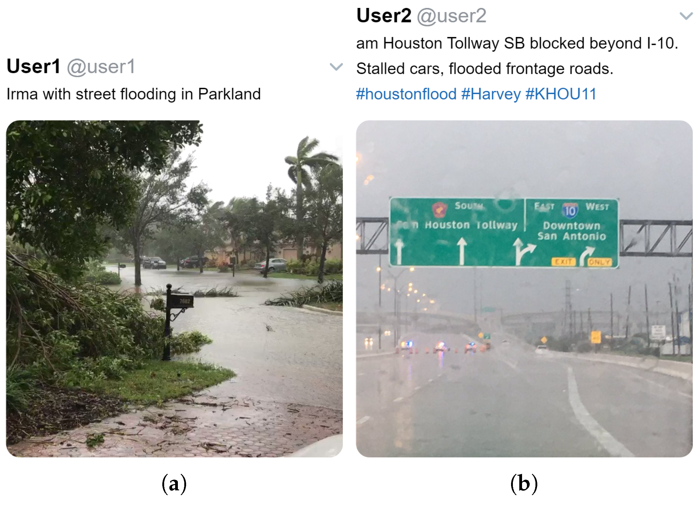
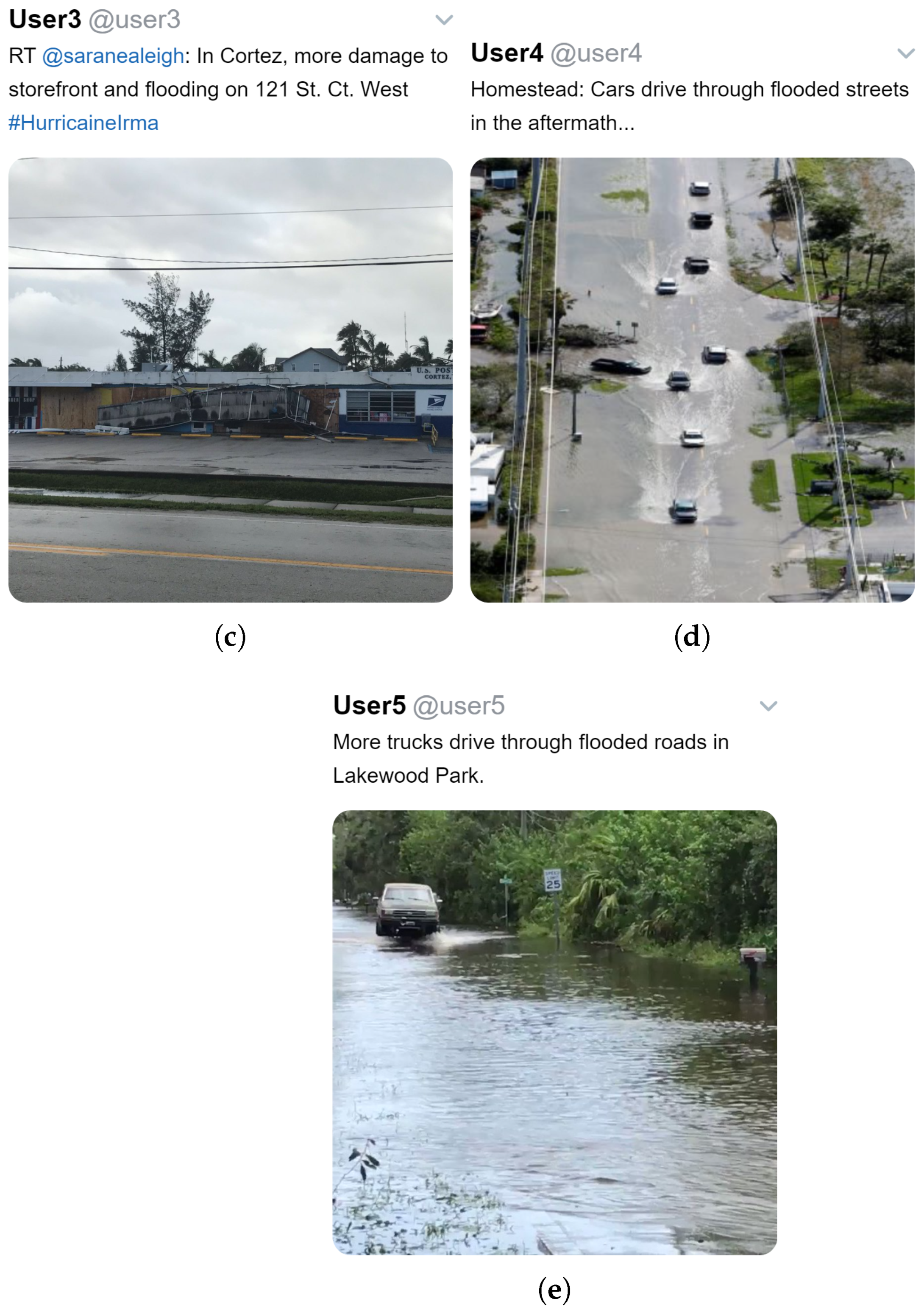
3.2. Images
4. Proposed Solutions
4.1. Algorithm Based on Metadata Only
4.2. Algorithms Based on Image Only
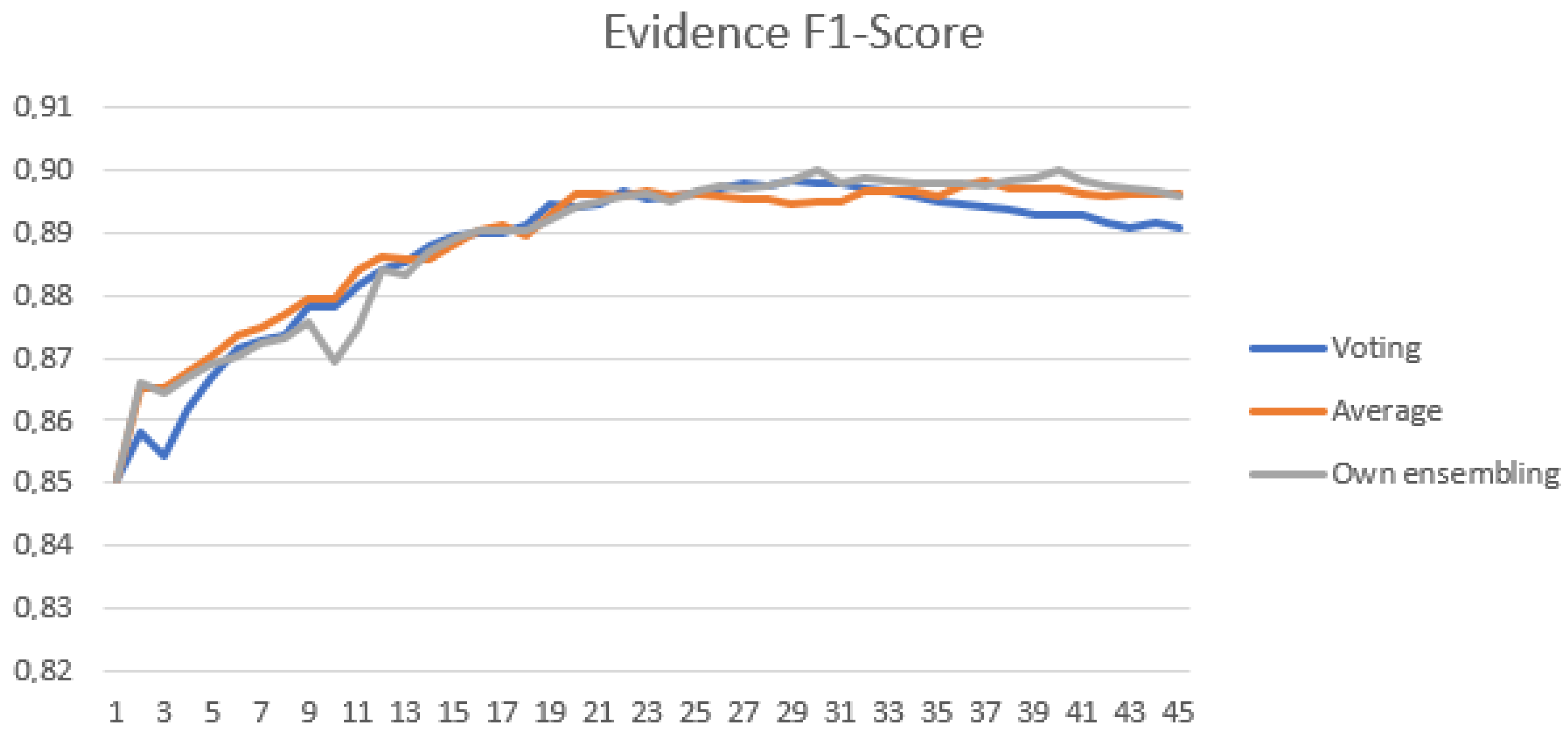
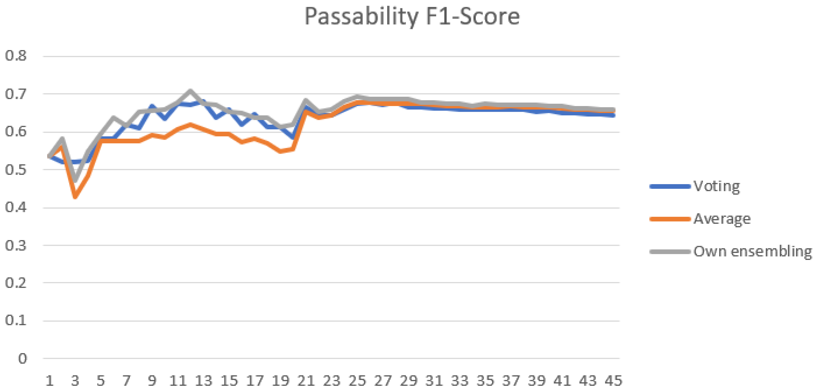
4.2.1. Ensemble Image Base Architecture
4.2.2. Double-Ended Network
4.2.3. Compactness Loss
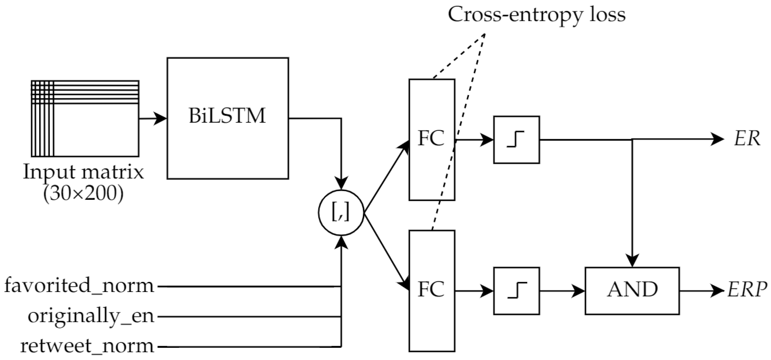
4.3. Algorithm Based on Metadata and Visual Information
5. Evaluation and Results
5.1. Results Using Metadata Only
5.2. Results Using Images Only
5.3. Results Using Images and Metadata
6. Conclusions
Author Contributions
Funding
Acknowledgments
Conflicts of Interest
Appendix A
References
- EM-DAT. The International Disaster Database; Centre of Research on the Epidemiology of Disasters—CRED: Brussels, Belgium, 2019. [Google Scholar]
- EM-DAT. The International Disaster Database—Data Access; Centre of Research on the Epidemiology of Disasters—CRED: Brussels, Belgium, 2019. [Google Scholar]
- EU-Commission. Funding Opportunities to Support Disaster Risk Prevention in the Cohesion Policy 2014–2020 Period; European Commission: Brussels, Belgium, 2014. [Google Scholar]
- AnsuR Technologies AS. UN-ASIGN. 2019. App. Available online: https://play.google.com/store/apps/details?id=ansur.asign.un&hl=en_US (accessed on 4 November 2020).
- AnsuR Technologies AS. UN-ASIGN. 2019. FP7 Project. Available online: https://cordis.europa.eu/project/rcn/94375/factsheet/en (accessed on 4 November 2020).
- Istituto Superiore Mario Boella (ISMB). I-REACT. 2019. App. Available online: https://play.google.com/store/apps/details?id=it.ismb.iReact&hl=en_US (accessed on 4 November 2020).
- Istituto Superiore Mario Boella (ISMB). I-REACT. 2019. H2020 Project. Available online: https://cordis.europa.eu/project/rcn/203294/factsheet/en (accessed on 4 November 2020).
- Wukich, C. Social media use in emergency management. J. Emerg. Manag. 2015, 13, 281–294. [Google Scholar] [CrossRef] [PubMed]
- Lopez-Fuentes, L.; Farasin, A.; Skinnemoen, H.; Garza, P. Deep Learning Models for Passability Detection of Flooded Roads; CEUR-WS: Aachen, Germany, 2018; p. 2283. [Google Scholar]
- Saroj, A.; Pal, S. Use of social media in crisis management: A survey. Int. J. Disaster Risk Reduct. 2020, 48, 101584. [Google Scholar] [CrossRef]
- Kankanamge, N.; Yigitcanlar, T.; Goonetilleke, A.; Kamruzzaman, M. Determining disaster severity through social media analysis: Testing the methodology with South East Queensland Flood tweets. Int. J. Disaster Risk Reduct. 2020, 42, 101360. [Google Scholar] [CrossRef]
- Kankanamge, N.; Yigitcanlar, T.; Goonetilleke, A. How engaging are disaster management related social media channels? The case of Australian state emergency organisations. Int. J. Disaster Risk Reduct. 2020, 48, 101571. [Google Scholar] [CrossRef]
- Ferner, C.; Havas, C.; Birnbacher, E.; Wegenkittl, S.; Resch, B. Automated Seeded Latent Dirichlet Allocation for Social Media Based Event Detection and Mapping. Information 2020, 11, 376. [Google Scholar] [CrossRef]
- Kruspe, A.; Kersten, J.; Klan, F. Detection of informative tweets in crisis events. Nat. Hazards Earth Syst. Sci. Discuss. 2020, 1–18. [Google Scholar] [CrossRef]
- Lopez-Fuentes, L.; van de Weijer, J.; Bolanos, M.; Skinnemoen, H. Multi-modal Deep Learning Approach for Flood Detection. MediaEval 2017, 17, 13–15. [Google Scholar]
- Zaffaroni, M.; Rossi, C. Water Segmentation with Deep Learning Models for Flood Detection and Monitoring. In Proceedings of the 17th ISCRAM Conference, Blacksburg, VA, USA, 24–27 May 2020; pp. 66–74. [Google Scholar]
- Lopez-Fuentes, L.; Rossi, C.; Skinnemoen, H. River segmentation for flood monitoring. In Proceedings of the 2017 IEEE International Conference on Big Data (Big Data), Orlando, FL, USA, 6–10 November 2017; pp. 3746–3749. [Google Scholar]
- Bînă, D.; Vlad, G.A.; Onose, C.; Cercel, D.C. Flood Severity Estimation in News Articles Using Deep Learning Approaches; CEUR-WS: Aachen, Germany, 2019; p. 2670. [Google Scholar]
- Zaffaroni, M.; Lopez-Fuentes, L.; Farasin, A.; Garza, P.; Skinnemoen, H. AI-Based Flood Event Understanding and Quantification Using Online Media and Satellite Data; CEUR-WS: Aachen, Germany, 2019; p. 2670. [Google Scholar]
- Feng, Y.; Shebotnov, S.; Brenner, C.; Sester, M. Ensembled Convolutional Neural Network Models for Retrieving Flood Relevant Tweets. In Proceedings of the MediaEval 2018 Workshop, Sophia Antipolis, France, 29–31 October 2018. [Google Scholar]
- Hanif, M.; Atif Tahir, M.; Rafi, M. Detection of passable roads using Ensemble of Global and Local Features. In Proceedings of the MediaEval 2018 Workshop, Sophia Antipolis, France, 29–31 October 2018. [Google Scholar]
- Moumtzidou, A.; Giannakeris, P.; Andreadis, S.; Mavropoulos, A.; Meditskos, G.; Gialampoukidis, I.; Avgerinakis, K.; Vrochidis, S.; Kompatsiaris, I. A multimodal approach in estimating road passability through a flooded area using social media and satellite images. In Proceedings of the MediaEval 2018 Workshop, Sophia Antipolis, France, 29–31 October 2018. [Google Scholar]
- Kirchknopf, A.; Slijepcevic, D.; Zeppelzauer, M.; Seidl, M. Detection of Road Passability from Social Media and Satellite Images. In Proceedings of the MediaEval 2018 Workshop, Sophia Antipolis, France, 29–31 October 2018. [Google Scholar]
- Bojanowski, P.; Grave, E.; Joulin, A.; Mikolov, T. Enriching word vectors with subword information. Trans. Assoc. Comput. Linguist. 2017, 5, 135–146. [Google Scholar] [CrossRef] [Green Version]
- Mikolov, T.; Chen, K.; Corrado, G.; Dean, J. Efficient estimation of word representations in vector space. In Proceedings of the International Conference on Learning Representations (ICLR 2013), Scottsdale, AZ, USA, 2–4 May 2013; Available online: https://arxiv.org/pdf/1301.3781.pdf (accessed on 4 November 2020).
- Pennington, J.; Socher, R.; Manning, C. Glove: Global vectors for word representation. In Proceedings of the 2014 Conference on Empirical Methods in Natural Language Processing (EMNLP), Doha, Qatar, 25–29 October 2014; pp. 1532–1543. [Google Scholar]
- Bramer, M. Principles of Data Mining; Springer: Berlin, Germany, 2007; Volume 180. [Google Scholar]
- Kim, Y. Convolutional Neural Networks for Sentence Classification. In Proceedings of the 2014 Conference on Empirical Methods in Natural Language Processing (EMNLP); Association for Computational Linguistics: Doha, Qatar, 2014; pp. 1746–1751. [Google Scholar] [CrossRef] [Green Version]
- Chatzichristofis, S.A.; Boutalis, Y.S. CEDD: Color and edge directivity descriptor: A compact descriptor for image indexing and retrieval. In International Conference on Computer Vision Systems; Springer: Berlin, Germany, 2008; pp. 312–322. [Google Scholar]
- Jalab, H.A. Image retrieval system based on color layout descriptor and Gabor filters. In Proceedings of the 2011 IEEE Conference on Open Systems, Langkawi, Malaysia, 25–28 September 2011; pp. 32–36. [Google Scholar]
- Chatzichristofis, S.A.; Boutalis, Y.S. FCTH: Fuzzy color and texture histogram-a low level feature for accurate image retrieval. In Proceedings of the IEEE 2008 Ninth International Workshop on Image Analysis for Multimedia Interactive Services, Klagenfurt, Austria, 7–9 May 2008; pp. 191–196. [Google Scholar]
- Park, D.K.; Jeon, Y.S.; Won, C.S. Efficient use of local edge histogram descriptor. In Proceedings of the 2000 ACM Workshops on Multimedia; ACM: New York, NY, USA, 2000; pp. 51–54. [Google Scholar]
- Zagoris, K.; Chatzichristofis, S.A.; Papamarkos, N.; Boutalis, Y.S. Automatic image annotation and retrieval using the joint composite descriptor. In Proceedings of the IEEE2010 14th Panhellenic Conference on Informatics, Tripoli, Greece, 10–12 September 2010; pp. 143–147. [Google Scholar]
- Manjunath, B.S.; Ohm, J.R.; Vasudevan, V.V.; Yamada, A. Color and texture descriptors. IEEE Trans. Circuits Syst. Video Technol. 2001, 11, 703–715. [Google Scholar] [CrossRef] [Green Version]
- Krizhevsky, A.; Sutskever, I.; Hinton, G.E. ImageNet classification with deep convolutional neural networks. Adv. Neural Inf. Process. Syst. 2012, 25, 1097–1105. [Google Scholar] [CrossRef]
- Huang, G.; Liu, Z.; Van Der Maaten, L.; Weinberger, K.Q. Densely connected convolutional networks. In Proceedings of the IEEE Conference on Computer Vision and Pattern Recognition, Honolulu, HI, USA, 21–26 July 2017; pp. 4700–4708. [Google Scholar]
- Szegedy, C.; Vanhoucke, V.; Ioffe, S.; Shlens, J.; Wojna, Z. Rethinking the inception architecture for computer vision. In Proceedings of the IEEE Conference on Computer Vision and Pattern Recognition, Las Vegas, NV, USA, 27–30 June 2016; pp. 2818–2826. [Google Scholar]
- Szegedy, C.; Ioffe, S.; Vanhoucke, V.; Alemi, A.A. Inception-V4, Inception-ResNet and the impact of residual connections on learning. In Proceedings of the Thirty-First AAAI Conference on Artificial Intelligence, San Francisco, CA, USA, 4–9 February 2017. [Google Scholar]
- He, K.; Zhang, X.; Ren, S.; Sun, J. Deep residual learning for image recognition. In Proceedings of the IEEE Conference on Computer Vision and Pattern Recognition, Las Vegas, NV, USA, 27–30 June 2016; pp. 770–778. [Google Scholar]
- Simonyan, K.; Zisserman, A. Very Deep Convolutional Networks for Large-Scale Image Recognition. International Conference on Learning Representations. 2015. Available online: https://www.robots.ox.ac.uk/~vgg/publications/2015/Simonyan15/simonyan15.pdf (accessed on 4 November 2020).
- Redmon, J.; Farhadi, A. YOLOv3: An Incremental Improvement. arXiv 2018, arXiv:1804.02767. [Google Scholar]
- Deng, J.; Dong, W.; Socher, R.; Li, L.J.; Li, K.; Fei-Fei, L. ImageNet: A large-scale hierarchical image database. In Proceedings of the 2009 IEEE Conference on Computer Vision and Pattern Recognition, Miami, FL, USA, 20–25 June 2009; pp. 248–255. [Google Scholar]
- Zhou, B.; Lapedriza, A.; Khosla, A.; Oliva, A.; Torralba, A. Places: A 10 million image database for scene recognition. IEEE Trans. Pattern Anal. Mach. Intell. 2018, 40, 1452–1464. [Google Scholar] [CrossRef] [PubMed] [Green Version]
- Girshick, R.; Donahue, J.; Darrell, T.; Malik, J. Rich feature hierarchies for accurate object detection and semantic segmentation. In Proceedings of the IEEE Conference on Computer Vision and Pattern Recognition, Columbus, OH, USA, 23–28 June 2014; pp. 580–587. [Google Scholar]
- Bischke, B.; Helber, P.; Dengel, A. Global-Local Feature Fusion for Image Classification of Flood Affected Roads from Social Multimedia. In Proceedings of the MediaEval 2018 Workshop, Sophia Antipolis, France, 29–31 October 2018. [Google Scholar]
- Zhao, Z.; Larson, M.; Oostdijk, N. Exploiting Local Semantic Concepts for Flooding-related Social Image Classification. In Proceedings of the MediaEval 2018 Workshop, Sophia Antipolis, France, 29–31 October 2018. [Google Scholar]
- Dias, D.; Dias, U. Flood detection from social multimedia and satellite images using ensemble and transfer learning with CNN architectures. In Proceedings of the MediaEval 2018 Workshop, Sophia Antipolis, France, 29–31 October 2018. [Google Scholar]
- Said, N.; Pogorelov, K.; Ahmad, K.; Riegler, M.; Ahmad, N.; Ostroukhova, O.; Halvorsen, P.; Conci, N. Deep learning approaches for flood classification and flood aftermath detection. In Proceedings of the MediaEval 2018 Workshop, Sophia Antipolis, France, 29–31 October 2018. [Google Scholar]
- MediaEval 2018 Multimedia Satellite Task. 2018. Available online: http://www.multimediaeval.org/mediaeval2018/multimediasatellite/ (accessed on 31 May 2018).
- Bischke, B.; Helber, P.; Zhao, Z.; de Bruijn, J.; Borth, D. The Multimedia Satellite Task at MediaEval 2018: Emergency Response for Flooding Events. In Proceedings of the MediaEval 2018 Workshop, Sophia Antipolis, France, 29–31 October 2018. [Google Scholar]
- Wang, P.; Qian, Y.; Soong, F.K.; He, L.; Zhao, H. Learning distributed word representations for Bidirectional LSTM recurrent neural network. In Proceedings of the 2016 Conference of the North American Chapter of the Association for Computational Linguistics: Human Language Technologies, San Diego, CA, USA, 12–17 June 2016; pp. 527–533. [Google Scholar]
- Lerman, P. Fitting segmented regression models by grid search. J. R. Stat. Soc. Ser. C (Appl. Stat.) 1980, 29, 77–84. [Google Scholar] [CrossRef]
- Liu, X.; Liang, D.; Yan, S.; Chen, D.; Qiao, Y.; Yan, J. Fots: Fast oriented text spotting with a unified network. In Proceedings of the IEEE Conference on Computer Vision and Pattern Recognition, Salt Lake City, UT, USA, 18–23 June 2018; pp. 5676–5685. [Google Scholar]
- Selvaraju, R.R.; Cogswell, M.; Das, A.; Vedantam, R.; Parikh, D.; Batra, D. Grad-CAM: Visual explanations from deep networks via gradient-based localization. In Proceedings of the IEEE International Conference on Computer Vision, Venice, Italy, 22–29 October 2017; pp. 618–626. [Google Scholar]
- Perera, P.; Patel, V.M. Learning deep features for one-class classification. IEEE Trans. Image Process. 2019, 28, 5450–5463. [Google Scholar] [CrossRef] [PubMed] [Green Version]


| Dataset | # Tot. Imgs | # Evid. of Roads | # Passable Roads | ||
|---|---|---|---|---|---|
| YES | NO | YES | NO | ||
| development set | 5818 | 2130 | 3688 | 951 | 1179 |
| test set | 3017 | - | - | - | - |
| Field | Description | Type |
|---|---|---|
| Created at | UTC time when this tweet was created | object |
| Entities | Dictionary of the entities which have been parsed out of the text, such as the hashtags | object |
| Extended entities | Dictionary of entities extracted from the media, such as the image size | object |
| Favorite count | Indicates how many times the tweet has been liked | int64 |
| Favorited | Indicates whether the tweet has been liked | bool |
| Id | Unique identifier of the tweet | int64 |
| Id str | String version of the unique identifier | object |
| Is quote status | Indicates whether this is a quoted tweet | bool |
| Lang | Indicates the language of the text (machine generated) | object |
| Possibly sensitive | When the tweet contains a link it indicates if the content of the URL is identified as containing sensitive content | object |
| Retweet count | Indicates how many times has the tweet been retweeted | int64 |
| Retweeted | Indicates whether the tweet has been retweeted | bool |
| Source | Utility used to post the tweet | object |
| text | Text written by the user | object |
| Truncated | Whether the value of the text parameter was truncated | bool |
| User | Dictionary of information about the user who posted the tweet | object |
| Approach\Data | Evidence of Road [%] | Ev. of Road Passability [%] | ||
|---|---|---|---|---|
| Validation Set | Test Set | Validation Set | Test Set | |
| Human annotation | 51.48 ** | - | 18.18 ** | - |
| Metadata only | 59.93 | 62.56 * | 56.82 | 57.05 * |
| Y. Feng et al. [20] | - | - | - | 32.8 |
| M. Hanif et al. [21] | - | 58.30 | - | 31.15 |
| Z. Zhao et al. [46] | - | 32.60 | - | 12.86 |
| A. Moumtzidou et al. [22] | - | - | - | 30.17 |
| A. Kirchknopf et al. [23] | - | - | - | 20 |
| Approach\Data | Evidence of Road [%] | Ev. of Road Passability [%] | ||||
|---|---|---|---|---|---|---|
| Validation Set | Test Set | Test Set | Validation Set | Test Set | Test Set | |
| (MediaEval) | (Own) | (MediaEval) | (Own) | |||
| Human annotation | 87.32 * | - | - | 47.71 * | - | - |
| Ensemble image base architecture (90) | 90.14 | 87.79 | 90.17 | 64.33 | 68.38 | 65.91 |
| Ensemble image base architecture (30) | 88.91 | - | 89.45 | 70.18 | - | 65.28 |
| Single network image base architecture | 86.48 | - | 84.88 | 62.84 | - | 59.99 |
| Double-ended architecture | 88.73 | - | 85.00 | 67.51 | - | 67.91 |
| Double-ended with compactness loss | 87.78 | - | 86.42 | 67.49 | - | 68.53 |
| Y. Feng et al. [20] | - | - | - | - | 64.35 | - |
| M. Hanif et al. [21] | - | 74.58 | - | - | 45.04 | - |
| Z. Zhao et al. [46] | - | 87.58 | - | - | 63.13 | - |
| A. Moumtzidou et al. [22] | - | - | - | - | 66.65 | - |
| A. Kirchknopf et al. [23] | - | - | - | - | 24 | - |
| N. Said et al. [48] | - | - | - | - | 65.03 | - |
| D. Dias [47] | - | - | - | - | 64.81 | - |
| B. Bischke [45] | - | 87.70 | - | - | 66.48 | - |
| Approach\Data | Evidence of Road [%] | Ev. of Road Passability [%] | ||
|---|---|---|---|---|
| Validation Set | Test Set | Validation Set | Test Set | |
| Double-ended architecture | 78.96 | 86.99 * | 61.06 | 62.96 * |
| Double-ended with compactness loss | 77.85 | 84.56 * | 73.61 | 75.93 * |
| Y. Feng et al. [20] | - | - | - | 59.49 |
| M. Hanif et al. [21] | - | 76.61 | - | 45.56 |
| Z. Zhao et al. [46] | - | 87.58 | - | 63.88 |
| A. Moumtzidou et al. [22] | - | - | - | 66.43 |
| A. Kirchknopf et al. [23] | - | - | - | 35 |
Publisher’s Note: MDPI stays neutral with regard to jurisdictional claims in published maps and institutional affiliations. |
© 2020 by the authors. Licensee MDPI, Basel, Switzerland. This article is an open access article distributed under the terms and conditions of the Creative Commons Attribution (CC BY) license (http://creativecommons.org/licenses/by/4.0/).
Share and Cite
Lopez-Fuentes, L.; Farasin, A.; Zaffaroni, M.; Skinnemoen, H.; Garza, P. Deep Learning Models for Road Passability Detection during Flood Events Using Social Media Data. Appl. Sci. 2020, 10, 8783. https://0-doi-org.brum.beds.ac.uk/10.3390/app10248783
Lopez-Fuentes L, Farasin A, Zaffaroni M, Skinnemoen H, Garza P. Deep Learning Models for Road Passability Detection during Flood Events Using Social Media Data. Applied Sciences. 2020; 10(24):8783. https://0-doi-org.brum.beds.ac.uk/10.3390/app10248783
Chicago/Turabian StyleLopez-Fuentes, Laura, Alessandro Farasin, Mirko Zaffaroni, Harald Skinnemoen, and Paolo Garza. 2020. "Deep Learning Models for Road Passability Detection during Flood Events Using Social Media Data" Applied Sciences 10, no. 24: 8783. https://0-doi-org.brum.beds.ac.uk/10.3390/app10248783