Pose Estimation Utilizing a Gated Recurrent Unit Network for Visual Localization

Abstract

Lately, pose estimation based on learning-based Visual Odometry (VO) methods, where raw image data are provided as the input of a neural network to get 6 Degrees of Freedom (DoF) information, has been intensively investigated. Despite its recent advances, learning-based VO methods still perform worse than the classical VO that consists of feature-based VO methods and direct VO methods. In this paper, a new pose estimation method with the help of a Gated Recurrent Unit (GRU) network trained by pose data acquired by an accurate sensor is proposed. The historical trajectory data of the yaw angle are provided to the GRU network to get a yaw angle at the current timestep. The proposed method can be easily combined with other VO methods to enhance the overall performance via an ensemble of predicted results. Pose estimation using the proposed method is especially advantageous in the cornering section which often introduces an estimation error. The performance is improved by reconstructing the rotation matrix using a yaw angle that is the fusion of the yaw angles estimated from the proposed GRU network and other VO methods. The KITTI dataset is utilized to train the network. On average, regarding the KITTI sequences, performance is improved as much as 1.426% in terms of translation error and 0.805 deg/100 m in terms of rotation error.

1. Introduction

Localization of a mobile robot and vehicle is a crucial factor needed for the development of autonomous robots and vehicles. While various localization methods have been developed, the abundance of information in images led to Visual Odometry (VO) based localization techniques, which were firstly carried out by Nister et al. [1]. Primarily, the VO estimates the pose of a rigid body incrementally by analyzing the changes that the motion of the rigid body induces on images collected by a camera [2].

Classical VO can be categorized into two types of methods, direct VO methods and feature-based VO methods, as depicted in Figure 1. Feature-based VO methods extract key feature points from the image (e.g., corners, edges, blobs) and match them into a sequential frame. These VO methods involve the ego-motion of the camera, which is estimated by minimizing reprojection errors between feature pairs obtained from sequential images. On the other hand, direct VO methods consist of dense VO methods using all pixels, semi-dense VO methods using pixels with sufficiently large intensity gradient, and sparse VO methods utilizing sparsely selected pixels. In direct VO methods, the ego-motion of the camera is estimated by minimizing the photometric error with non-linear optimization algorithms [3,4].

For each type of method, various techniques have been investigated to increase the accuracy of the VO. In case of feature-based VO methods, which are considered the mainstream of the VO, many studies focus on outlier rejection and finding appropriate features to track for decrement of the error of the VO [6,7,8]. To get better results of pose estimation, Patruno et al. presented a robust correspondence feature filter relying on statistical and geometrical information [9]. Learning-based feature detectors are also investigated. In [10], Yi et al. proposed an integrated feature extraction pipeline, called Learned Invariant Feature Transform (LIFT) pipeline, consisting of a detector, orientation estimator, and descriptor. In [11], DeTone et al. presented neural network architecture for point detection, which is trained by using a self-supervised domain adaptation called Homographic Adaptation. In [12], Revaud et al. proposed the Repeatable and Reliable Detector and Descriptor (R2D2) which is a new learning-based feature extraction method. The R2D2 can learn repeatability and reliability of each key point. In [13], a hierarchical localization technique is introduced, employing Hierarchical Feature Network (HF-Net) based on monolithic Convolutional Neural Network (CNN) which efficiently predicts hierarchical features.

For direct VO methods, to solve the main drawback of feature-based VO methods fundamentally relying on features, pixel-to-pixel direct matching methods with assumption of constant brightness in optical flow are also studied. Despite this adjustment, the feature-based VO methods have been regarded as more suitable approaches than the direct VO methods for cases involving large baselines, fast motions, and varied illumination [14,15,16,17,18,19,20]. From this perspective, studies to combine the advantages of direct VO methods and feature-based VO methods to decrease errors of VO have been conducted [20,21].

Recently, the application of Deep Neural Networks (DNNs) for the VO has been intensively investigated [22,23,24,25,26]. Most of the applications of DNNs is for learning-based VO methods. In [22], Kendall et al. presented a real-time re-localization system using Deep Convnet consisting of CNNs. Since VO is a continuation of sequential estimation, architectures such as Recurrent Neural Network (RNN), Long Short-Term Memory (LSTM) network, and Gated Recurrent Unit (GRU) network can be adopted. In [23], Wang et al. proposed a learning-based Monocular Visual Odometry (MVO) with the help of deep Recurrent Convolutional Neural Network (RCNN). In [24], VO approach using a dual-stream neural network consisting of a CNN and an LSTM network is proposed by Lit et al. Liu et al. presented an MVO system employing RCNN [25]. In [26], Zhao et al. proposed Learning Kalman Network for improved learning of dynamically changing parameters during end-to-end training for VO without specifying parameters explicitly. In learning-based VO methods, structures of feature-based VO methods and direct VO methods are replaced with the fine-tuned DNNs, however, results of the KITTI benchmark test show that the performances of learning-based VO methods have not yet surpassed the performances of the classical VO (e.g., feature-based VO methods, direct VO methods). For this reason, hybrid methods making use of classical VO combined with learning-based VO are studied in [27,28]. In [27], Peretroukhin et al. proposed a Deep Pose Correction (DPC) network consisting of CNNs. The DPC network predicts camera motion correction according to stereo images. A classical VO framework is fused with the DPC network by Pose Graph Relaxation. In [28], pose estimation relying on the combined use of classical VO with DNNs is presented with camera motion estimated by pre-processed optical flow images.

Despite foregoing efforts, many problems in the VO remain unsolved. Imaging conditions (e.g., sunlight, shadows, image blur) fundamentally affect the performance of the VO [4]. To overcome the problems that occurred by change of light source, various approaches have been attempted. For instance, learning-based detectors (e.g., R2D2, SuperPoint [11]) have proven to be superior to non-machine learning detectors (e.g., Speeded-Up Robust Features, Scale Invariant Feature Transform). When the camera rotates (e.g., yaw rotation), a large change of pixels in the image occurs as compared to that due to translation. The large change of pixels in the image quickly reduces the lifespan of the feature points when using feature-based VO methods, and also causes large rotation error and translation error in learning-based VO methods as well as classical VO [29,30,31,32]. Furthermore, the learning-based VO methods require tremendous time for learning, due to its usage of images to train the network.

This work introduces a correction method for the VO by using prior driving data generated from a relatively accurate sensor such as Real-Time Kinematic Global Positioning System (RTK-GPS) which has 0.02 m/0.1 deg resolution [33]. The performance of the correction method is not affected by the characteristics of images. Being inspired by the trend of using a learning-based VO and classical VO together, this work presents a pose estimation that uses a GRU network which is an improved version of RNN and computationally more efficient than the LSTM network [34,35]. The GRU network is trained by historical trajectory data of the yaw angle constrained by the shape and structure of a robot or a vehicle. The GRU network receives the stacked yaw angles converted from 6 Degrees of Freedom (DoF) as the input, which is the result of classical VO, and predicts the next yaw angle. The 2 yaw angles, one obtained from the GRU network and the other obtained from the classical VO, are fused together. The simulation is conducted with a VO adopting a MVO framework.

The main contributions of this paper are summarized as follows

• A VO based on GRU network is proposed for predicting future yaw angle by making use of stacked yaw angle obtained from classical VO.
• The proposed method is able to extract rotational tendency constrained by shape or type of robot or vehicle, particularly effective in the cornering section.
• A modified VO framework is developed to improve VO performance by applying the GRU network to the classical VO without causing any change of the pipeline of the original VO.
• Fusion of yaw angle by Normalized Cross-Correlation (NCC) and subsequent reconstruction of the rotation matrix by using the fused yaw angle are presented.

For performance comparison, the KITTI dataset [33] often used in the development of VO is utilized.

The rest of this paper is organized as follows. Section 2 describes the process of MVO, error analysis during camera rotation, and structure of GRU network for predicting yaw angle. Section 3 presents how to train and test the GRU network and gives consequential simulation results obtained from the use of GRU network. Section 4 concludes this paper.

2. System Overview

2.1. Visual Odometry

The process of the feature-based VO method is shown in Figure 2. Features are detected by feature detectors such as Smallest Univalue Segment Assimilating Nucleus (SUSAN) and Features from Accelerated Segment Test (FAST). The detected feature points are tracked in sequential frames. Local optimization to obtain optimized pose can be executed by sparse bundle adjustment. The VO dealt with in this work is 2D-to-2D motion estimation involved with rotation and translation. The pipeline of the VO in Figure 2 can be described by the pseudo-code in Algorithm 1.

Algorithm 1 Pseudo-code of Monocular Visual Odometry algorithm [2,36]. 2D-to-2D Monocular Visual Odometry

Capture images: $I_{k-1}$, $I_k$ Undistort the images $I_{k-1}$, $I_k$ Use FAST algorithm to detect features in $I_{k-1}$, and match those features to $I_k$, A new detection is triggered if the number of features falls below threshold. Use Nister’s 5-point algorithm with RANSAC [37] to compute the essential matrix. Estimate $R$, $t$ from the essential matrix that was computed in the previous step. Take scale information from ground truth data and concatenate the translation vector and rotation matrix. Repeat from line 1.

In 2D-to-2D VO, the transformation $T_k=\left[\begin{array}{cc}R& t\\ 0& 1\end{array}\right]\in {ℝ}^{4\times 4}$ is estimated in a way that minimizes reprojection error $\underset{T_k}{argmin}\sum _i\parallel P_k^i-{\widehat{P}}_{k-1}^i{\parallel }^2$ where $T_k$ represents motion estimation between two images $I_{k-1}$, $I_k$ obtained with a calibrated camera, and ${\widehat{p}}_{k-1}^i$ = $f\left(T_k,X^i{}_{k-1}\right)$ represents the reprojection of corresponding feature point $X^i{}_{k-1}$ onto image $I_k$ following transformation $T_k$ by reprojection function $f(\cdot )$. Furthermore, $p_k^i$ is the observed feature point in the current frame $I_k$.

The essential matrix $E$ defined according to the rotation matrix $R\in SO\left(3\right)$ where $SO\left(3\right)=\{R\in {ℝ}^{3\times 3}|R{R}^T=I,\det (R)=1\}$ and the translation vector $t\in {ℝ}^3$ is given as follows

$$E=\widehat{t}R$$

(1)

where the translation vector is defined as $t=\left[\begin{array}{c}{t}_x\\ t_y\\ t_z\end{array}\right]$ and the skew-symmetric matrix of the translation vector $t$ is defined as $\widehat{t}=\left[\begin{array}{ccc}0& -t_z& t_y\\ t_z& 0& -t_x\\ -t_y& t_x& 0\end{array}\right]$. Furthermore, the essential matrix $E$ can be represented by Singular Value Decomposition (SVD) as follows

$$E=U\Sigma V^T$$

(2)

where $U$ is the unitary matrix, $\sum$ is the orthogonal matrix, and $V^T$ is the transpose of conjugate matrix. Then, the rotation matrix $R$ and $\widehat{t}$ can be extracted as follows

$$R=U\left(\pm W^{-1}\right)V^T,$$

(3)

$$\widehat{t}=U\left(\pm W\right)\Sigma U^T$$

(4)

where $W=\left[\begin{array}{ccc}0& \mp 1& 0\\ \pm 1& 0& 0\\ 0& 0& 1\end{array}\right]$. Among the possible 4 combinations in Equations (3) and (4), $R$ and $\widehat{t}$ are selected by judging whether the depth by the corresponding feature points is positive in both camera coordinate systems when the frame is $k-1$ and $k$. By getting the rotation matrix $R$, and the translation vector $t$, the ego-motion of the camera is estimated using the following equation

$$R_{traj,t}= R{R}_{traj,t-1},$$

(5)

$$t_{traj,t}=t_{traj,t-1}+\lambda \left(R_{traj,t-1}t\right)$$

(6)

where $\lambda$ is the scale information obtained from ground truth data. $R_{traj}$ and $t_{traj}$ are the accumulated rotation and translation calculated by the rotation matrix $R=\left(\begin{array}{ccc}{R}_{11}& R_{12}& R_{13}\\ R_{21}& R_{22}& R_{23}\\ R_{31}& R_{32}& R_{33}\end{array}\right)$ and the translation vector $t=\left[\begin{array}{c}{t}_x\\ t_y\\ t_z\end{array}\right]$.

2.2. Effect of Cornering on VO

Coordinate system and rotation of the camera around each axis are shown in Figure 3. In the VO, rotation around the y-axis (yaw) is the main component of rotation of robot and vehicle. Rotation of the camera in the x–z plane (yaw) result in large amount of change in the scene of the camera. It leads to tracking failure by changing the light source and causes large pixel change in the image. These are dramatically related to increasing photometric error and reprojection error. That is the main reason why increasing the accuracy of VO when the camera rotates in the x–z plane is crucial.

In the 2D-to-2D VO (i.e., Nister’s 5 point-based MVO) called MVO described in Algorithm 1, pitch angle ($\theta$), yaw angle ($\psi$), and roll angle ($\varphi$) are obtained as follows

$$\theta ,\psi ,\varphi =\{\begin{array}{cc}\theta =atan2\left(R_{32},R_{33}\right)& \\ \psi =atan2\left(-R_{31},\sqrt{R_{11}{R}_{11}+R_{21}{R}_{21}}\right)& if\parallel R^{T}R\parallel >k\\ \varphi =atan2\left(R_{21},R_{11}\right)& \\ & \\ \theta =atan2\left(-R_{23},R_{22}\right)& \\ \psi =atan2\left(-R_{31},\sqrt{R_{11}{R}_{11}+R_{21}{R}_{21}}\right)& otherwise\\ \varphi =0& \end{array}$$

(7)

where $R=\left(\begin{array}{ccc}{R}_{11}& R_{12}& R_{13}\\ R_{21}& R_{22}& R_{23}\\ R_{31}& R_{32}& R_{33}\end{array}\right)$ and $atan2(\cdot )$ is a function that returns arctangent value according to IEEE standard 754. The threshold $k$ is set to ${10}^{-6}$. To obtain Figure 4 representing the tendency of change in the yaw angle and the cumulative error of yaw angle, the absolute value of $\psi$, which corresponds to each pair of the images, is calculated. Then, the error $e$ is computed as follows

$$e=\sqrt{{\left({\psi }_{\mathrm{GT}}-{\psi }_{MVO}\right)}^2}$$

(8)

where ${\psi }_{GT}$ and ${\psi }_{MVO}$ are the yaw angles obtained with ground truth (GT) and MVO, respectively.

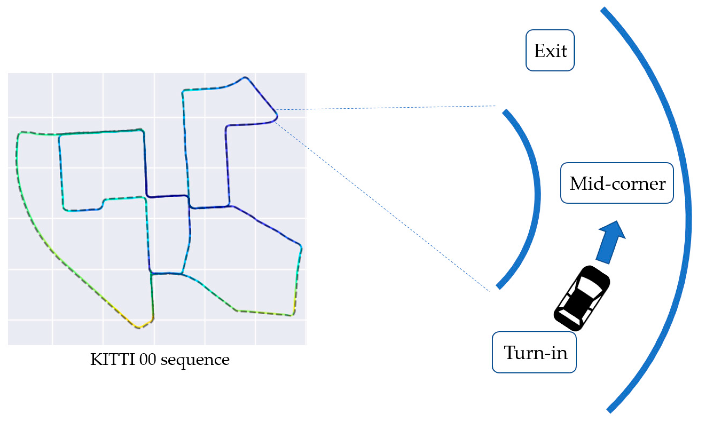
When the camera is rotated, the variation of the yaw angle calculated through the pair of images seems to be a bell shape that gradually increases and then decreases. In Figure 4, the starting point of increasing yaw angle is shown when the camera enters the cornering section (turn-in). The highest value of the yaw angle is shown when the camera is in the middle of the cornering section (mid-corner). Decrease of yaw angle is shown when the camera escapes from the cornering section (exit). The turn-in, mid-corner, and exit involved in a cornering section are shown in Figure 5. The accumulated error of the yaw angle is figured out to be rapidly increasing when the camera rotates and steadily increasing when sequence continues as shown in Figure 4. Note that the rotation is used for the calculation of $R_{traj}$ in Equation (5), and it is also used for calculation of $t_{traj}$ in Equation (6). Therefore, the method of increasing the accuracy in the cornering section can significantly improve the performance of VO.

2.3. Framework of Pose Estimation Utilizing GRU Network

2.3.1. Network Architecture

The proposed pose estimation method utilizes a GRU network shown in Figure 6a for predicting the yaw angle at the current timestep. The predicted yaw angle is to be used to minimize rotation error defined in x–z plane. In this study, sequential yaw angles obtained for the time interval $t_{-5}$ to $t_{-1}$ are applied as the network inputs and go through the GRU layers and then the prediction that corresponds to the yaw angle at $t_0$ is obtained through the output layer.

The GRU network consists of 5 GRU layers, each consisting of 5 GRU cells with 200 hidden units in each GRU cell, and 3 fully connected layers, each consisting of 256, 128, and 64 neurons. The structure of the GRU network architecture and GRU cell is shown in Figure 6a,b, respectively. The GRU network shown in Figure 6a consists of 25 (= 5 cells/layer $\times$ 5 layers) GRU cells, where 5 cells/layer represents the number of feature dimension (input dimension), in other words, the length of the input sequence. After the GRU layers, there are 3 fully connected layers before the final output layer that predicts the yaw angle. In the $l$-th GRU cell in Figure 6b, where $l=1,\dots ,5$, forward transfer formulation of GRU is calculated for each processing step as follows

$$r_t=\sigma \left(W_t\left[h_{t-1},x_t\right]+b_r\right),$$

(9)

$$z_t=\sigma \left(W_z\left[h_{t-1},x_t\right]+b_z\right),$$

(10)

$${\tilde{h}}_t=tanh(W_{\tilde{h}}\left[r_t\odot h_{t-1},x_t\right]+b_{\tilde{h}}),$$

(11)

$$h_t=\left(1-z_t\right)\odot h_{t-1}+z_t\odot {\tilde{h}}_t$$

(12)

where $r_t$ is the reset gate which determines how much information in the previous GRU cell should be forgotten and $z_t$ is the update gate which determines how much information should be transferred from the current GRU cell to the next GRU cell and ${\tilde{h}}_t$ is the intermediate state and $h_t$ is the hidden state and $\sigma (\cdot )$ is the sigmoid function and $tanh(\cdot )$ represents the hyperbolic tangent function and $W_r$, $W_z$, $W_{\tilde{h}}$ are entries of weight matrix $W$ and $b$ is bias vector and $\odot$ is element-wise multiplication. For the reset gate, large value of $r_t$ means much information from previous cell is forgotten. For the update gate, large value of $z_t$ means that much information is transferred to the next cell [34,39].

The 5 historical yaw angles estimated by the VO are the input to GRU layer at each time and the current output of each GRU cell is determined by both past and current inputs. A dropout layer is placed between each GRU layer to prevent overfitting. The overall structure is determined by a grid search to define the best hyperparameter values providing the best accuracy. The GRU network is trained by time series data, so continual training is required. The GRU network learns the cornering tendency in terms of yaw angle variation of the camera and then operates when the camera enters the cornering section so that it can predict the next yaw angle on cornering. This novel method can improve the performance of the VO by correcting the yaw angle estimation of the VO.

2.3.2. Framework with Classical VO

The proposed method is combined with a classical VO. The framework combining the classical VO and the proposed GRU network is shown in Figure 7. An image sequence is input to the classical VO and feature points are detected when the classical VO is a feature-based VO method. After detecting the feature points, feature matching (i.e., tracking) is conducted. As a result, the rotation matrix $R$ and the translation vector $t$ are obtained from the classical VO. In this process, a memory buffer containing the yaw angle for the last 5 timesteps is kept. If the camera enters the cornering section, the GRU network is activated and uses the previous 5 historical yaw angles obtained from the classical VO to predict the yaw angle for correcting the pose obtained from the classical VO.

To detect when the camera enters a cornering section, a process is defined as follows

$${\left|{\psi }_{VO}\right|}_{t = k-5,\dots ,k-1}\ge \gamma$$

(13)

where $\gamma$ is the threshold to check whether the camera is in the cornering section. The camera is determined to be in a cornering section when the yaw angles of the camera are continuously larger than the threshold angle $\gamma$. In this work, the threshold angle $\gamma$ is set to 0.85 deg through trial and error based on whether the cornering section could be well distinguished. It is recommended to set the threshold angle $\gamma$ slightly higher than the angle where the cornering section is well detected as will be discussed in the Section 3.1. The condition to identify when the estimated yaw angle from the classical VO deviates significantly from the previous rotation trend is defined as follows

$${\left|\frac{\Delta {\psi }_{VO}}{\Delta t}\right|}_{t = k}\ge \alpha max({\left|\frac{\Delta {\psi }_{VO}}{\Delta t}\right|}_{t = k-5,\dots ,k-1})$$

(14)

where $\alpha$ is scale factor determining the lower limit of the trend. The scale factor $\alpha$ for simulations is set to 1.5, considering the range of change allowed for variation of estimation by the classical VO in preliminary simulations. The condition to identify when the yaw angle estimated by the classical VO deviates from the yaw angle obtained from the GRU network is defined as follows

$${\left|\frac{\Delta {\psi }_{VO}}{\Delta t}\right|}_{t = k}\ge {\left|\frac{\Delta {\psi }_{GRU}}{\Delta t}\right|}_{t = k}.$$

(15)

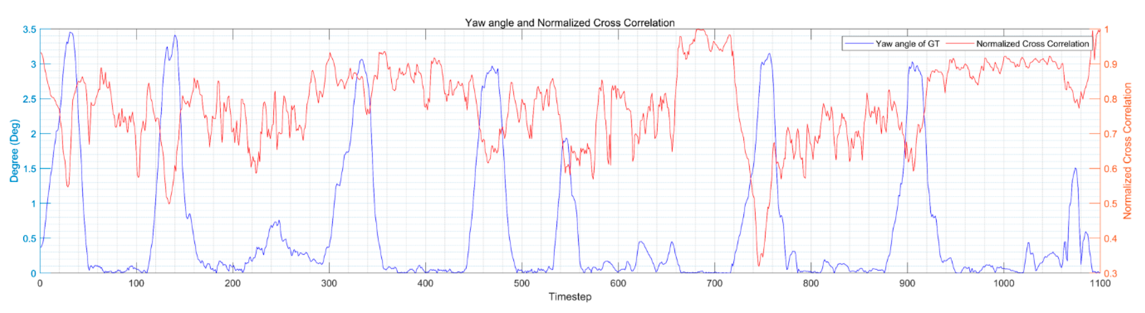
If the change of rotation is fairly large so that Equations (14) and (15) are satisfied, the yaw angle is corrected. Correction of yaw angle is executed by fusing the yaw angle obtained from the GRU network and the yaw angle obtained from the classical VO. The fusion is executed using the Normalized Cross-Correlation (NCC) as the weighting factor. The NCC represents the similarity between images and takes values between 0 and 1 [40]. The value of NCC rapidly decreases at the cornering section as shown in Figure 8. In addition, estimation by the classical VO becomes inaccurate at the cornering section as described in Section 2.2. The value of NCC can be considered as a reliability factor of the yaw angle calculated by the classical VO. In some sections with large NCC values, the proposed framework can trust less the estimated value by the GRU, thereby preventing possible problems of increased error when the GRU is fully trusted. Reconstruction of the rotation matrix is computed as follows

$$\begin{array}{l}{R}_{corr}=(\begin{array}{ccc}{R}_{11}& R_{12}& R_{13}\\ R_{21}& R_{22}& R_{23}\\ R_{31}& R_{32}& R_{33}\end{array})\\ =\left(\begin{array}{ccc}cos\theta cos\varphi & sin{\psi }_{corr}sin\theta cos\varphi -cos{\psi }_{corr}sin\varphi & cos{\psi }_{corr}sin\theta cos\varphi +sin{\psi }_{corr}sin\varphi \\ cos\theta sin\varphi & sin{\psi }_{corr}sin\theta sin\varphi +cos{\psi }_{corr}cos\varphi & cos{\psi }_{corr}sin\theta sin\varphi -sin{\psi }_{corr}cos\varphi \\ -sin\theta & sin\varphi cos\theta & cos\varphi cos\theta \end{array}\right)\end{array}$$

(16)

where ${\psi }_{corr}=NCC{\psi }_{VO}+\left(1-NCC\right){\psi }_{GRU}$ The NCC for the image $I_1$ centered on ($u$, $v$) and image $I_2$ centered on ($u^{\prime }$, $v^{\prime }$) is calculated with $m\times n$ patch, where $m=2a+1$, $n=2b+1$ are odd integers, as follows

$$NCC=\frac{{\sum }_{k=-a}^a{\sum }_{l=-b}^b\left[I_1\left(u+k,v+l\right)-{\mu }_1\right][I_2\left(u^{\prime }+k,v^{\prime }+l\right)-{\mu }_2]}{\sqrt{{\sum }_{k=-a}^a{\sum }_{l=-b}^b{[I_1\left(u+k,v+l\right)-{\mu }_1]}^2+{\sum }_{k=-a}^a{\sum }_{l=-b}^b{[I_2\left(u^{\prime }+k,v^{\prime }+l\right)-{\mu }_2]}^2}}$$

(17)

where

$$\begin{gathered} {\mu }_1=\frac{1}{\left(2a+1\right)\left(2b+1\right)}{\sum }_{k = -a}^a{\sum }_{l = -b}^b{I}_1\left(u+k,v+l\right), \\ {\mu }_2=\frac{1}{\left(2a+1\right)\left(2b+1\right)}{\sum }_{k = -a}^a{\sum }_{l = -b}^b{I}_2\left(u^{\prime }+k,v^{\prime }+l\right). \end{gathered}$$

The pseudo-code of the MVO based on the proposed pose estimation using the GRU network is shown in Algorithm 2. The 6-th line represents the condition for determining if the camera is in a cornering section and the 7-th line represents the condition for checking if the yaw angle from the VO deviates significantly from the previous rotation trend. In addition, in the 7-th line, the yaw angle is predicted by the GRU network and corrected using NCC and as a result the rotation matrix $R$ is reconstructed.

Algorithm 2 Pseudo-code of Monocular Visual Odometry algorithm based on proposed method. 2D-to-2D Monocular Visual Odometry with Pose Correction Using a GRU Network

Capture images: $I_{k-1}$, $I_k$ Undistort the images $I_{k-1}$, $I_k$ Use FAST algorithm to detect features in $I_{k-1}$, and match those features to $I_k$, A new detection is triggered if the number of features falls below threshold. Use Nister’s 5-point algorithm with RANSAC to compute the essential matrix. Estimate $R$, $t$ from the essential matrix that was computed in the previous step. If, all the absolute value of $\psi$ in the memory buffer ($\left|{\psi }_{k-5}\right|$, $\left|{\psi }_{k-4}\right|$, $\left|{\psi }_{k-3}\right|$, $\left|{\psi }_{k-2}\right|$, $\left|{\psi }_{k-1}\right|$) are larger than $\gamma$ for determining that the camera is in a cornering section go to 7. Else, go to 8. In this study, $\gamma$ is set to 0.85 deg. If ${\left|\frac{\Delta {\psi }_{VO}}{\Delta t}\right|}_{t = k}\ge \alpha max({\left|\frac{\Delta {\psi }_{VO}}{\Delta t}\right|}_{t = k-5,\dots ,k-1})and{\left|\frac{\Delta {\psi }_{VO}}{\Delta t}\right|}_{t = k}\ge {\left|\frac{\Delta {\psi }_{GRU}}{\Delta t}\right|}_{t = k}$ is satisfied, then, the yaw angle is corrected by ${\psi }_{corr}=NCC{\psi }_{VO}+\left(1-NCC\right){\psi }_{GRU}$ and $R$ is reconstructed using Equation (16). Else, go to 8. In this study, $\alpha$ is set to 1.5. Take scale information form ground truth data, and concatenate the translation vector, and the rotation matrix. Repeat from line 1.

3. Simulation

This section provides a concise and precise description of the training and testing of the proposed method as well as the analysis of simulation results. MATLAB® (R2020a, MathWorks, USA) is used to train and test the GRU network and Visual Studio® (2019, Microsoft Corporation, Redmond, CA, USA) and OpenCV 3.4.0 (Intel Ltd., Santa Clara, CA, USA) are used to simulate the VO. The GRU network trained in MATLAB® is linked with Visual Studio® using MEX, a function of MATLAB®. This process is carried out on a desktop PC with Intel® I7-9700KF (Intel Corporation, Santa Clara, CA, USA) and Nvidia® GPU RTX 2060 (NVIDIA Ltd., Santa Clara, CA, USA).

3.1. Training and Testing

To train the GRU network for predicting the yaw angle when a robot or a vehicle is in a cornering section, absolute values of the yaw angle obtained with ground truth data from RTK-GPS are used as the target values and absolute values of the yaw angle obtained from the MVO are taken as the input values. When the yaw angle of the robot or vehicle from RTK-GPS at time $t$ exceeds a certain threshold, the robot or vehicle is considered to be moving around a cornering section. If the vehicle is judged to be at a cornering section, the 2 yaw angles obtained by the MVO before time $t$ and another 2 yaw angles also obtained by the MVO after time $t$ are taken to form 5 historical yaw angles around time $t$. Note that the time $t$ is according to the RTK-GPS. Therefore, the dataset can be organized as follows

$$\begin{array}{l}\mathbb{X}=\left\{{\mathit{x}}_1,{\mathit{x}}_2,{\mathit{x}}_3\dots ,{\mathit{x}}_n\right\},\mathbb{Y}=\left\{y_1,y_2,y_3\dots ,y_n\right\}\\ \mathit{x}=\left(\left|{\psi }_{MVO,t-2}\right|,\left|{\psi }_{MVO,t-1}\right|,\left|{\psi }_{MVO,t}\right|,\left|{\psi }_{MVO,t+1}\right|,\left|{\psi }_{MVO,t+2}\right|\right),y=\left(\left|{\psi }_{RTK-GPS,t+3}\right|\right)\end{array}$$

(18)

where $\mathbb{X}$ is the set of feature vectors and $\mathbb{Y}$ is the set of target values and $\mathit{x}$ is a feature vector consisting of yaw angles and $y$ is a target value. The value for the sequential length is set to 5 after conducting ablation studies for the comparison of the final loss obtained for different values of the sequential length 3, 5, and 7. However, the sequential length can be adjusted depending on the characteristics of the system such as the frame rate of the camera. In this work, the threshold of the lower limit for $\left|{\psi }_t\right|$ is set to 0.8 deg and, if the yaw angle exceeds 0.8 deg, the corners can be extracted as shown in Figure 9. This threshold must be set carefully as it may vary depending on the hardware constraints of the robot or vehicle and resolution and type of the sensor.

The training set consists of 4811 training sequences obtained from the MVO and the ground truth of KITTI dataset consisting of 11 sequences with indices 00–10. Then, 80% of training sequences sare used for training of the GRU network and the remaining 20% are used for network validation (testing). The GRU network is trained using Adam optimizer [41]. The training of the GRU network is done similarly to regression. In other words, The GRU network is trained to reduce the loss $ℒ=\frac{1}{n}{\sum }_{i = 1}^n{(f_{\theta }\left({\mathit{x}}_i\right)-y_i)}^2$ where $f_{\theta }\left({\mathit{x}}_i\right)$ is the prediction of the GRU network. Both the output of the network and the ground truth yaw angle values are real numbers. The model at the epoch with the minimum value of the loss $ℒ$ is chosen as the best model for the simulations in the Section 3.2. The minibatch size is set to 32 during training.

3.2. Evaluation

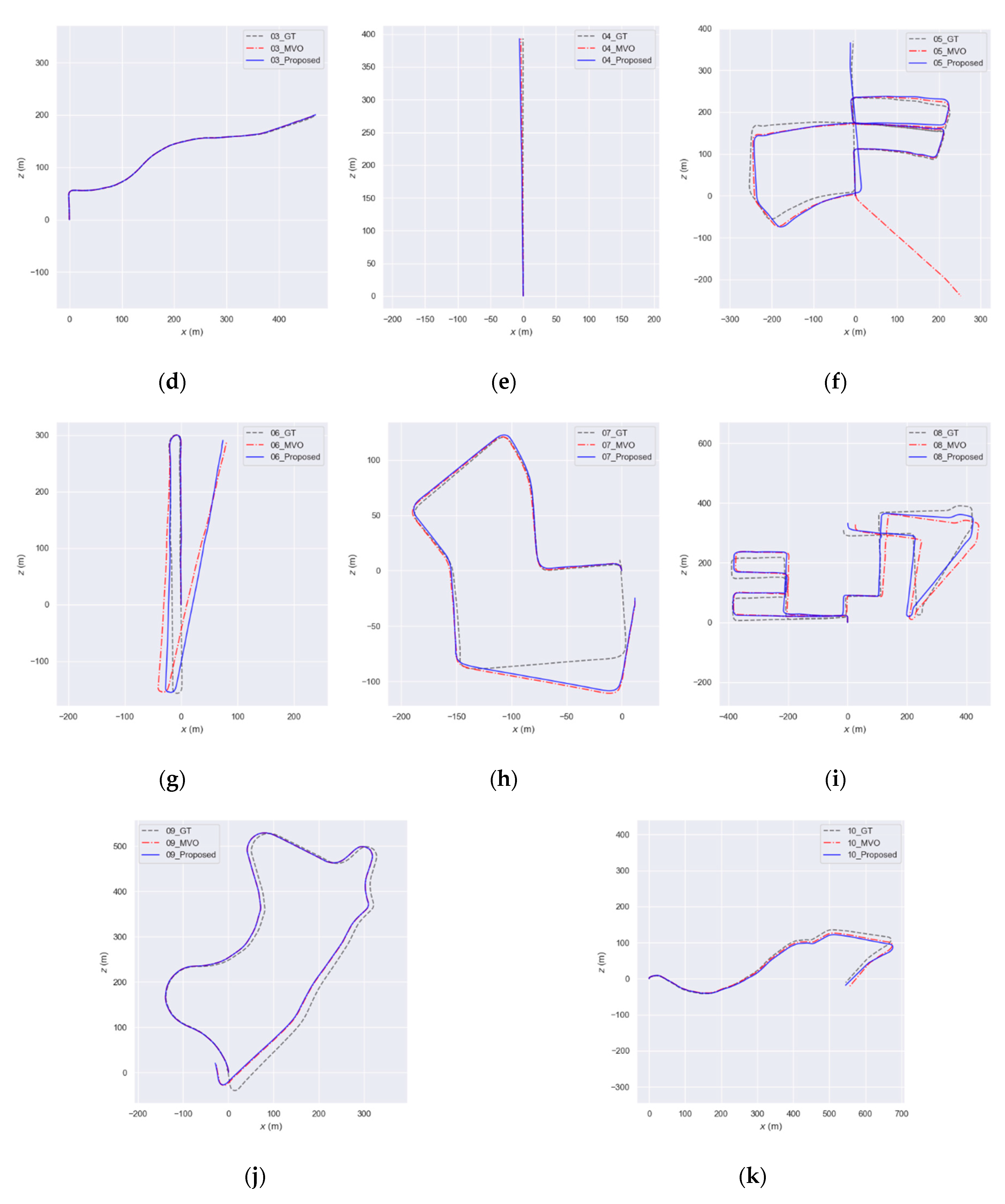
In Figure 10, the accumulated Root Mean Square Errors (RMSEs) concerning yaw angle obtained from the MVO framework employing the proposed method are reduced when comparing with the MVO. The yaw angle obtained from the MVO employing the proposed method is closer to ground truth than the MVO, as shown in enlarged timesteps of Figure 10a corresponding to the cornering section of the KITTI 06 sequence over timesteps 710–730. For the section where the proposed method is applied, the yaw angle from the proposed method is closer to ground truth as depicted in Figure 11. The timesteps over which the green line segments are overlayed correspond to the timesteps when yaw angle changes. In addition, as seen in Figure 12, it is intuitively clear that odometry performance is improved over the trajectories of most sequences in the KITTI dataset.

The KITTI evaluation kit [42,43] is used for the evaluations in this subsection. In

Table 1. Simulation results obtained for the KITTI sequences 00 to 10. The value marked in red is the amount of reduced error.

Sequence			00	01	02	03	04	05	06	07	08	09	10	Avg
MVO	Tr [%]	Err	11.307	6.174	11.819	5.165	0.641	16.745	4.384	8.032	11.427	8.554	6.199	8.222
	Rot [deg /100 m]	Err	3.946	2.171	4.688	2.597	0.373	10.444	2.118	5.427	3.770	2.885	5.17	3.963
	ATE [m]	Err	143.731	38.289	90.335	1.545	0.232	128.369	26.280	15.427	88.199	28.789	8.642	51.803
	RPE [m]	Err	0.022	0.176	0.026	0.022	0.026	0.018	0.025	0.021	0.028	0.024	0.018	0.037
	RPE [deg]	Err	0.311	0.275	0.284	0.222	0.063	0.346	0.153	0.221	0.253	0.260	0.321	0.246
MVO + Proposed method	Tr [%]	Err	9.769	6.201	10.767	5.135	0.738	5.524	4.396	8.106	9.678	8.564	5.886	6.797
		Diff	−1.538	0.027	−1.052	−0.030	0.097	−11.221	0.012	0.074	−1.749	0.010	−0.313	−1.426
	Rot [deg /100 m]	Err	3.554	2.268	4.384	2.597	0.406	2.794	1.960	5.496	3.422	2.889	4.968	3.158
		Diff.	−0.392	0.097	−0.304	0.000	0.033	−7.650	−0.158	0.069	−0.348	0.004	−0.202	−0.805
	ATE [m]	Err	121.600	38.096	79.475	1.545	0.177	39.750	25.882	14.665	72.799	28.937	6.643	39.052
		Diff.	−22.131	−0.193	−10.860	0.000	−0.055	−88.619	−0.398	−0.762	−15.400	0.148	−1.999	−12.752
	RPE [m]	Err	0.023	0.179	0.026	0.022	0.026	0.018	0.025	0.020	0.027	0.024	0.019	0.037
		Diff.	0.001	0.003	0.000	0.000	0.000	0.000	0.000	−0.001	−0.001	0.000	0.001	0.000
	RPE [deg]	Err	0.306	0.282	0.279	0.222	0.063	0.206	0.152	0.221	0.247	0.259	0.318	0.232
		Diff.	−0.005	0.007	−0.005	0.000	0.000	−0.140	−0.001	0.000	−0.006	−0.001	−0.003	−0.014
Deep VO [45]	Tr [%]	Err	65.749	138.875	11.819	81.133	20.053	47.975	70.602	62.13	72.711	90.195	110.799	70.186
	Rot [deg/ 100 m]	Err	28.745	11.612	4.688	30.119	7.19	28.675	29.824	50.996	30.599	25.633	25.814	24.900

, translation error [44], rotation error [44], Absolute Trajectory Error (ATE) [43], and Relative Pose Error (RPE) [43] are presented for demonstrating the performance improvement achieved with the proposed method.

Assuming that the sequence of spatial poses from the estimated trajectory is $P_i$ and the sequence of spatial poses from the ground truth is $Q_i$ and $S$ is the rigid body transformation, the absolute trajectory error matrix at time $i$ is given as follows

$$e_i=Q_i{}^{-1}S{P}_i.$$

(19)

Then, the ATE is defined as follows

$$ATE=\sqrt{(\frac{1}{n}{\displaystyle \sum }_{i = 1}^n\Vert trans\left(e_i\right){\Vert }^2)}$$

(20)

where $trans\left(\left[\begin{array}{cc}R& t\\ 0& 1\end{array}\right]\right)=t$. The function $trans(\cdot )$ extracts $t$ using $T=\left[\begin{array}{cc}R& t\\ 0& 1\end{array}\right]$ as an input parameter. In addition, the relative pose error matrix at time $i$ over a fixed time interval $△$ is given as follows

$$F_i^{△}={(Q_i{}^{-1}{Q}_{i+△})}^{-1}\left(P_i{}^{-1}{P}_{i+△}\right).$$

(21)

The RPE for translation $RP{E}_{trans}$ and rotation $RP{E}_{rot}$ are defined as follows

$$RP{E}_{trans}^{i,\Delta }=\sqrt{(\frac{1}{m}{\sum }_{i = 1}^m\Vert trans\left(F_i\right){\Vert }^2)},$$

(22)

$$RP{E}_{rot}^{i,\Delta }=\frac{1}{m}{\sum }_{i = 1}^m\angle \left(rot\left(F_i{}^{\Delta }\right)\right)$$

(23)

where $rot\left(\left[\begin{array}{cc}R& t\\ 0& 1\end{array}\right]\right)=R$. The function $rot(\cdot )$ extracts $R$ using $T=\left[\begin{array}{cc}R& t\\ 0& 1\end{array}\right]$ as an input parameter and $\angle R=arccos(\frac{trace\left(R\right)-1}{2})$ where $trace(\cdot )$ is the sum of components on main diagonal of square matrix.

Table 1 shows the simulation results obtained for the KITTI sequences 00 to 10. The values corresponding to ‘Diff’ in Table 1 are the values obtained by subtracting the error value of the MVO from the error value obtained with the proposed method. The value marked in red is the amount of improvement. With the proposed method, the translation error is decreased with KITTI sequences 00, 02, 03, 05, 08, 10 as compared to the MVO. The rotation error is decreased with KITTI sequences 00, 02, 05, 06, 08, 10. The ATE (m) is decreased with KITTI sequences 00, 01, 02, 04, 05, 06, 07, 08, 10.

The RPE (m) is decreased with KITTI sequences 07, 08, and unchanged with KITTI sequences 02, 03, 04, 05, 06, 09. The RPE (deg) is decreased with KITTI sequences 00, 02, 05, 06, 08, 09, 10. On average, errors of all metrics except the RPE (m) are reduced. For the RPE (m) metric, the performance obtained with the proposed method is similar to the classical MVO. On average, the translation error is reduced as much as 1.426% and the rotation error is decreased as much as 0.805 deg/100 m and the ATE is reduced as much as 12.752 m, and the RPE is decreased as much as 0.014 deg. Using the hybrid method for yaw correction, the DPC-Net [27] combining learning-based VO with the classical VO, for the KITTI 00, 02, and 05 sequences, 30.06% improvement of translation error and 24.98% enhancement of rotation error can be achieved as compared to the classical VO. Comparing proposed method with the DPC-Net, the proposed method for the KITTI 00, 02, and 05 sequences demonstrates 34.64% improvement of translation error and 43.75% enhancement of rotation error as compared to the classical VO. However, the RPE (deg) for KITTI sequence 01 is slightly increased as much as 0.007 deg. This is due to incorrect estimation with the GRU network in the timestep when the estimated value by the classical VO is significantly different from the previous rotation tendency. The increment of RPE can be solved by fine-tuning the GRU network and adjusting the parameters $\alpha$, $\gamma$.

In Table 1, the comparison with the Deep VO [23], that is one of the learning-based VO methods, is presented. The results shown in Table 1 are indicative of the better performance of the classical VO than the Deep VO.

4. Conclusions

In this paper, a pose estimation method utilizing a GRU network is proposed. The GRU network predicts yaw angles based on sequential yaw angle data. The predicted yaw angle is used in the proposed method for yaw angle correction at the cornering section where rotational error and translation error tend to increase. The GRU network is trained by the sequences of yaw angle data at the cornering section obtained from the classical VO and an accurate sensor. During testing of the GRU network, the next yaw angle is predicted by the GRU network taking the yaw angles estimated by the classical VO as the input. In this way, more accurate yaw angle is obtained by fusing the yaw angles estimated by the classical VO and the GRU network with NCC as the weighing factor of the fusion mechanism. With the estimated yaw angle, the rotation matrix is reconstructed for subsequent use.

Simulation results with 11 sequences of the KITTI dataset show that with the classical VO employing the proposed method, the performances in terms of translation error and rotation error are improved significantly. In addition, the proposed method requires less computational effort for learning when compared with the learning-based VO using images as the input data. Since the proposed method is combined with the classical VO without any change in the original pipeline, the proposed method can be applied to various VO methods. The proposed method can be applied not only to feature-based VO methods, as for the simulations conducted in this paper, but also to direct and learning-based VO methods. The proposed method suggests that the prediction based on the GRU network can improve the performance in unstable areas such as cornering section.

References

- Nistér, D.; Naroditsky, O.; Bergen, J. Visual odometry. In Proceedings of the 2004 IEEE Computer Society Conference on Computer Vision and Pattern Recognition, Washington, DC, USA, 27 June–2 July 2004. [Google Scholar]
- Scaramuzza, D.; Fraundorfer, F. Visual odometry [tutorial]. IEEE Robot. Autom. Mag. 2011, 18, 80–92. [Google Scholar] [CrossRef]
- Li, R.; Wang, S.; Gu, D. Ongoing evolution of visual slam from geometry to deep learning: Challenges and opportunities. Cognit. Comput. 2018, 10, 875–889. [Google Scholar] [CrossRef]
- Yang, N.; Wang, R.; Gao, X.; Cremers, D. Challenges in monocular visual odometry: Photometric calibration, motion bias, and rolling shutter effect. IEEE Robot. Autom. Lett. 2018, 3, 2878–2885. [Google Scholar] [CrossRef] [Green Version]
- Sun, R.; Giuseppe, B.A. 3D Reconstruction of Real Environment from Images Taken from UAV (SLAM Approach). Ph.D. Thesis, Politecnico di Torino, Turin, Italy, 2018. [Google Scholar]
- Cvišić, I.; Petrović, I. Stereo odometry based on careful feature selection and tracking. In Proceedings of the 2015 European Conference on Mobile Robots (ECMR), Paris, France, 2–4 September 2015; pp. 1–6. [Google Scholar]
- More, R.; Kottath, R.; Jegadeeshwaran, R.; Kumar, V.; Karar, V.; Poddar, S. Improved pose estimation by inlier refinement for visual odometry. In Proceedings of the 2017 Third International Conference on Sensing, Signal Processing and Security (ICSSS), Chennai, India, 4–5 May 2017; pp. 224–228. [Google Scholar]
- Liu, Y.; Gu, Y.; Li, J.; Zhang, X. Robust stereo visual odometry using improved RANSAC-based methods for mobile robot localization. Sensors 2017, 17, 2339. [Google Scholar] [CrossRef] [PubMed] [Green Version]
- Patruno, C.; Colella, R.; Nitti, M.; Renò, V.; Mosca, N.; Stella, E. A Vision-Based Odometer for Localization of Omnidirectional Indoor Robots. Sensors 2020, 20, 875. [Google Scholar] [CrossRef] [PubMed] [Green Version]
- Yi, K.M.; Trulls, E.; Lepetit, V.; Fua, P. Lift: Learned invariant feature transform. In Proceedings of the European Conference on Computer Vision, Amsterdam, The Netherlands, 8–16 October 2016; pp. 467–483. [Google Scholar]
- DeTone, D.; Malisiewicz, T.; Rabinovich, A. Superpoint: Self-supervised interest point detection and description. In Proceedings of the IEEE Conference on Computer Vision and Pattern Recognition Workshops, Salt Lake City, UT, USA, 18–22 June 2018; pp. 224–236. [Google Scholar]
- Revaud, J.; Weinzaepfel, P.; De Souza, C.; Pion, N.; Csurka, G.; Cabon, Y.; Humenberger, M. R2d2: Repeatable and reliable detector and descriptor. arXiv 2019, arXiv:1906.06195. [Google Scholar]
- Sarlin, P.-E.; Cadena, C.; Siegwart, R.; Dymczyk, M. From coarse to fine: Robust hierarchical localization at large scale. In Proceedings of the 2019 IEEE Conference on Computer Vision and Pattern Recognition, Long Beach, CA, USA, 15–19 June 2019; pp. 12716–12725. [Google Scholar]
- Newcombe, R.A.; Lovegrove, S.J.; Davison, A.J. DTAM: Dense tracking and mapping in real-time. In Proceedings of the 2011 International Conference on Computer Vision, Barcelona, Spain, 7–13 November 2011; pp. 2320–2327. [Google Scholar]
- Engel, J.; Schöps, T.; Cremers, D. LSD-SLAM: Large-scale direct monocular SLAM. In Proceedings of the 2014 European Conference on Computer Vision, Zurich, Switzerland, 6–12 September 2014; pp. 834–849. [Google Scholar]
- Caruso, D.; Engel, J.; Cremers, D. Large-scale direct SLAM for omnidirectional cameras. In Proceedings of the 2015 IEEE/RSJ International Conference on Intelligent Robots and Systems (IROS), Hamburg, Germany, 28 September–2 October 2015; pp. 141–148. [Google Scholar]
- Engel, J.; Stückler, J.; Cremers, D. Large-scale direct SLAM with stereo cameras. In Proceedings of the 2015 IEEE/RSJ International Conference on Intelligent Robots and Systems (IROS), Hamburg, Germany, 28 September–2 October 2015; pp. 1935–1942. [Google Scholar]
- Usenko, V.; Engel, J.; Stückler, J.; Cremers, D. Direct visual-inertial odometry with stereo cameras. In Proceedings of the 2016 IEEE International Conference on Robotics and Automation (ICRA), Stockholm, Sweden, 16–21 May 2016; pp. 1885–1892. [Google Scholar]
- Wang, R.; Schworer, M.; Cremers, D. Stereo DSO: Large-scale direct sparse visual odometry with stereo cameras. In Proceedings of the 2017 IEEE International Conference on Computer Vision, Venice, Italy, 22–29 October 2017; pp. 3903–3911. [Google Scholar]
- Zhao, X.; Liu, L.; Zheng, R.; Ye, W.; Liu, Y. A robust stereo feature-aided semi-direct SLAM system. Robot. Auton. Syst. 2020, 132, 103597. [Google Scholar] [CrossRef]
- Wang, F.; Lü, E.; Wang, Y.; Qiu, G.; Lu, H. Efficient Stereo Visual Simultaneous Localization and Mapping for an Autonomous Unmanned Forklift in an Unstructured Warehouse. Appl. Sci. 2020, 10, 698. [Google Scholar] [CrossRef] [Green Version]
- Kendall, A.; Grimes, M.; Cipolla, R. Posenet: A convolutional network for real-time 6-dof camera relocalization. In Proceedings of the 2015 IEEE International Conference on Computer Vision, Las Condes, Chile, 11–18 December 2015; pp. 2938–2946. [Google Scholar]
- Wang, S.; Clark, R.; Wen, H.; Trigoni, N. Deepvo: Towards end-to-end visual odometry with deep recurrent convolutional neural networks. In Proceedings of the 2017 IEEE International Conference on Robotics and Automation (ICRA), Singapore, 29 May–3 June 2017; pp. 2043–2050. [Google Scholar]
- Liu, Q.; Zhang, H.; Xu, Y.; Wang, L. Unsupervised Deep Learning-Based RGB-D Visual Odometry. Appl. Sci. 2020, 10, 5426. [Google Scholar] [CrossRef]
- Liu, Q.; Li, R.; Hu, H.; Gu, D. Using unsupervised deep learning technique for monocular visual odometry. IEEE Access 2019, 7, 18076–18088. [Google Scholar] [CrossRef]
- Zhao, C.; Sun, L.; Yan, Z.; Neumann, G.; Duckett, T.; Stolkin, R. Learning Kalman Network: A deep monocular visual odometry for on-road driving. Robot. Auton. Syst. 2019, 121, 103234. [Google Scholar] [CrossRef]
- Peretroukhin, V.; Kelly, J. Dpc-net: Deep pose correction for visual localization. IEEE Robot. Autom. Lett. 2017, 3, 2424–2431. [Google Scholar] [CrossRef] [Green Version]
- Peretroukhin, V.; Wagstaff, B.; Giamou, M.; Kelly, J. Probabilistic regression of rotations using quaternion averaging and a deep multi-headed network. arXiv 2019, arXiv:1904.03182. [Google Scholar]
- Comport, A.I.; Malis, E.; Rives, P. Real-time quadrifocal visual odometry. Int. J. Robot. Res. 2010, 29, 245–266. [Google Scholar] [CrossRef] [Green Version]
- Gutierrez, D.; Rituerto, A.; Montiel, J.; Guerrero, J.J. Adapting a real-time monocular visual slam from conventional to omnidirectional cameras. In Proceedings of the 2011 IEEE International Conference on Computer Vision Workshops (ICCV Workshops), Barcelona, Spain, 6–13 November 2011; pp. 343–350. [Google Scholar]
- Wang, S.; Clark, R.; Wen, H.; Trigoni, N. End-to-end, sequence-to-sequence probabilistic visual odometry through deep neural networks. Int. J. Robot. Res. 2018, 37, 513–542. [Google Scholar] [CrossRef]
- Jiao, J.; Jiao, J.; Mo, Y.; Liu, W.; Deng, Z. MagicVO: An End-to-End hybrid CNN and bi-LSTM method for monocular visual odometry. IEEE Access 2019, 7, 94118–94127. [Google Scholar] [CrossRef]
- Geiger, A.; Lenz, P.; Stiller, C.; Urtasun, R. Vision meets robotics: The kitti dataset. Int. J. Robot. Res. 2013, 32, 1231–1237. [Google Scholar] [CrossRef] [Green Version]
- Zhu, J.; Yang, Z.; Guo, Y.; Zhang, J.; Yang, H. Short-term load forecasting for electric vehicle charging stations based on deep learning approaches. Appl. Sci. 2019, 9, 1723. [Google Scholar] [CrossRef] [Green Version]
- Yang, S.; Yu, X.; Zhou, Y. LSTM and GRU Neural Network Performance Comparison Study: Taking Yelp Review Dataset as an Example. In Proceedings of the 2020 International Workshop on Electronic Communication and Artificial Intelligence (IWECAI), Shanghai, China, 12–14 June 2020; pp. 98–101. [Google Scholar]
- Singh, A.; Venkatesh, K. Monocular Visual Odometry. Undergrad. Proj 2. 2015. Available online: http://avisingh599.github.io/assets/ugp2-report.pdf (accessed on 11 December 2020).
- Fischler, M.A.; Bolles, R.C. Random sample consensus: A paradigm for model fitting with applications to image analysis and automated cartography. Commun. ACM 1981, 24, 381–395. [Google Scholar] [CrossRef]
- Grupp, M. Python Package for the Evaluation of Odometry and SLAM. Available online: https://libraries.io/pypi/evo (accessed on 2 November 2020).
- Ouyang, H.; Zeng, J.; Li, Y.; Luo, S. Fault Detection and Identification of Blast Furnace Ironmaking Process Using the Gated Recurrent Unit Network. Processes 2020, 8, 391. [Google Scholar] [CrossRef] [Green Version]
- Siegwart, R.; Nourbakhsh, I.R.; Scaramuzza, D. Introduction to Autonomous Mobile Robots; MIT Press: Cambridge, MA, USA, 2011. [Google Scholar]
- Kingma, D.P.; Ba, J. Adam: A method for stochastic optimization. arXiv 2014, arXiv:1412.6980. [Google Scholar]
- Zhan, H. kitti-Odom-Eval. Available online: https://github.com/Huangying-Zhan/kitti-odom-eval (accessed on 15 September 2020).
- Prokhorov, D.; Zhukov, D.; Barinova, O.; Anton, K.; Vorontsova, A. Measuring robustness of Visual SLAM. In Proceedings of the 2019 16th International Conference on Machine Vision Applications (MVA), Tokyo, Japan, 27–31 May 2019; pp. 1–6. [Google Scholar]
- Geiger, A.; Lenz, P.; Urtasun, R. Are we ready for autonomous driving? In The kitti vision benchmark suite. In Proceedings of the 2012 IEEE Conference on Computer Vision and Pattern Recognition, Providence, RI, USA, 16–21 June 2012; pp. 3354–3361. [Google Scholar]
- ChiWeiHsiao; Daiyk; Alexander. DeepVO-Pytorch. Available online: https://github.com/ChiWeiHsiao/DeepVO-pytorch (accessed on 15 September 2020).
Figure 1.
The process of Visual Odometry (VO) methods: (a) feature-based VO method and (b) direct VO method [5].
Figure 2.
Pipeline (process) of feature-based VO method [2].
Figure 3.
Camera coordinate system.
Figure 4.
Accumulated yaw angle error and yaw angles of ground truth (GT) and camera calculated by Monocular Visual Odometry (MVO) with KITTI 06, 08, and 09 sequences. (a) The KITTI sequence 06. (b) The KITTI sequence 08. (c) The KITTI sequence 09. The left y-axis is for the yaw angle and the right y-axis is for the accumulated yaw angle error.
Figure 5.
Turn-in, mid-corner, and exit involved with a cornering section [38].
Figure 6.
Architecture of Gated Recurrent Unit (GRU) network for predicting yaw angle and GRU cell. (a) GRU network. (b) A GRU cell where × is element-wise multiplication.
Figure 7.
Proposed pose estimation framework with classical VO.
Figure 8.
Camera yaw angle calculated by MVO and Normalized Cross-Correlation (NCC) of each pair of frames for the KITTI 07 sequence. The left vertical axis represents the yaw angle and the right vertical axis is the NCC.
Figure 9.
Ground truth trajectory from RTK-GPS (Real-Time Kinematic Global Positioning System) of KITTI 06 sequence; the red trajectory is the section where the yaw angle exceeds the threshold and the green trajectory corresponds to the remaining section where the yaw angle falls below the threshold.
Figure 10.
Accumulated yaw angle error and yaw angle of ground truth (GT) and camera calculated by the MVO and the MVO with the proposed method with KITTI 06, 08, and 09 sequences. (a) The KITTI sequence 06. (b) The KITTI sequence 08. (c) The KITTI sequence 09. The left vertical axis is for the yaw angle and the right vertical axis is for the accumulated yaw angle error.
Figure 11.
Enlarged cornering section of ground truth (GT), yaw angle obtained from the MVO, and yaw angle obtained from the MVO employing the proposed method when KITTI 06, 08, and 09 sequences are used. (a) KITTI sequence 06 over timesteps 670–740 is depicted. (b) KITTI sequence 08 over timesteps 1290–1340 is depicted. (c) KITTI sequence 09 over timesteps 1480–1560 is depicted.
Figure 12.
Trajectory of KITTI sequences 00 to 10 about ground truth (GT), MVO, MVO with the proposed method (00 to 10 sequence in alphabetical order (a–k)).